DOI:10.32604/cmc.2022.019314
| Computers, Materials & Continua DOI:10.32604/cmc.2022.019314 | |
| Article |
Deterministic and Stochastic Fractional-Order Hastings-Powell Food Chain Model
1Department of Mathematics, Unaizah College of Sciences and Arts, Qassim University, Unaizah, 51911, Saudi Arabia
2Department of Mathematics, Buraydah College of Sciences and Arts, Qassim University, Buraydah, 51431, Saudi Arabia
*Corresponding Author: Moustafa El-Shahed. Email: elshahedm@yahoo.com
Received: 09 April 2021; Accepted: 11 June 2021
Abstract: In this paper, a deterministic and stochastic fractional-order model of the tri-trophic food chain model incorporating harvesting is proposed and analysed. The interaction between prey, middle predator and top predator population is investigated. In order to clarify the characteristics of the proposed model, the analysis of existence, uniqueness, non-negativity and boundedness of the solutions of the proposed model are examined. Some sufficient conditions that ensure the local and global stability of equilibrium points are obtained. By using stability analysis of the fractional-order system, it is proved that if the basic reproduction number
Keywords: Food chain model; global dynamics; stability; stochastic; Hastings-Powell model; harvesting
Mathematical analysis is one of the important tools for understanding and interpreting different interactions in the environment around us. The food chain model system is attractive to researchers in theoretical ecology because it helps to understand the relationships between populations and describe the behavior of the ecosystem. Hastings et al. [1] investigated a three-species food chain model with Holling type II functional responses. Hastings-Powell model, has been revisited recently by many authors [2–16]. In the real world, food chain models are always affected by environmental noise. Thus, the stochastic models may be a more appropriate way of modeling the Hastings-Powell food chain model in many circumstances [17,18]. Recently, fractional calculus has been applied to describe different mathematical models, and it has been shown to be more accurate in some cases compared to the classical models [19–26]. The main objective of this paper is to study the deterministic and stochastic fractional-order Hastings-Powell model incorporating harvesting. This model is an extension of the classical Hastings-Powell model (1) by introducing fractional derivative, stochastic and harvesting. The qualitative behavior of the proposed model is investigated. Also, a numerical approximation method is developed for the proposed stochastic fractional-order model.
The paper is arranged as follows: In Section 2, the mathematical model is described. Some preliminary results, such as existence, uniqueness, nonnegativity and boundedness are presented in Section 3. The local and global stability of equilibrium points of the fractional-order food chain model is analyzed in Section 4. With the help of Sotomayor’s theorem, the transcritical bifurcation of the proposed model is investigated in Section 5. Section 6 extends the deterministic fractional- order food chain model to the stochastic fractional-order model. In Section 7, some numerical simulations are presented to verify the obtained theoretical results. Finally, the conclusions are given in Section 8.
Recently, Nath et al. [27] studied the following system of integer order differential equations to understand the underlying dynamics of the food chain model:
with initial values
In the above model
Introducing dimensionless
Making the above substitutions in the model (1). Then the system yields the following form
The dimensionless parameters in the food chain model (2) are defined as
Following [13,15,16], by replacing the integer derivative by a Caputo fractional derivative in (2), one can obtain the following fractional-order system
where,
In this section, the existence and uniqueness of the solutions of the fractional-order system (3) are investigate in the region
for sufficiently large
Theorem 1. For each
Proof. Define a mapping
For any
where
Hence,
3.2 Non-Negativity and Boundedness
The following results show the non-negativity of the solutions of the fractional-order system (3). According to [28], a model of the form
Theorem 2. All the solutions of the fractional-order food chain Model (3) starting in
Proof. The approach of [29,30] is utilized. Let
where,
where
Hence all the solutions of fractional-order a tri-trophic food chain model (3) that start in
One can also prove that
The fractional-order system (3) has the following equilibrium points:
1)
2) The middle predator and top predator free equilibrium point
3) Following [32],
4) The top predator extinction equilibrium point
5) The top predator extinction equilibrium point
6) The coexistence positive equilibrium point
7) and
The locally and globally asymptotically stable of equilibrium points of fractional-order food chain model (3) are now investigated. The Jacobian matrix is given as follows:
The eigenvalues of
Theorem 3. If
Proof. The Jacobian matrix of model (3) at
The eigenvalues of
Theorem 4. If
Proof. Let us consider the following positive definite Lyapunov function
The time derivative of
According to Theorem 1,
Choosing
According to generalized Lyapunov–Lasalle’s invariance principle [33],
Hence the equilibrium point
The global stability of the equilibrium point
when
The stability of top predator extinction equilibrium point
Theorem 5. If
Proof. The Jacobian matrix of model (3) at
where
The above equation has the following eigenvalue
Theorem 6. If
Proof. The following positive definite Lyapunov function is considered.
By calculating the time derivative of
Choosing
The stability of coexistence equilibrium point
Theorem 7. If
Proof. The Jacobian matrix of model (3) at
where
where
If we choose
Following [34], it is interested to note that the function
has a similar effect as the real part of the eigenvalue in the integer order system. If
Theorem 8. If
Proof. Let us consider the function
By calculating the time derivative of
Choosing
In this section we will investigate the local bifurcation near the free predator equilibrium point of the food chain model (2) with the help of Sotomayor’s theorem [35] to discuss the bifurcation analysis of the underlying system. The food chain model (2) can be rewritten in a vector form
Theorem 9. The food chain model (2) undergoes a transcritical bifurcation with respect to the bifurcation parameter
Proof. The Jacobian matrix of the food chain model (2) at the free predator equilibrium point
The eigenvector corresponding to
then
Thus, according to Sotomayor’s theorem, the food chain model (2) has a transcritical bifurcation at
6 Stochastic Fractional-order Model
This section extends the deterministic fractional-order food chain model (3) to the following stochastic fractional-order model.
where
where
According to [36–39], under some conditions on the coefficient functions, the global existence and uniqueness of solutions for the stochastic fractional-order system (13) can be investigated. Because Grunwald-Letnikov’s definition is the most straightforward from the point of view of numerical implementation, so one can use it to solve the Hastings-Pwoell system of fractional-order stochastic differential equations. Grunwald-Letnikov (
where
where
If
Now, the fractional-order stochastic Hastings-Pwoell model (11) in Grunwald-Letnikov sense can be written as
where,
In this part, the numerical simulations of the mathematical model (3) will be examined, and the focus will be on the effect of harvesting parameters. The numerical results will be compared with the theorems formulated in the previous sections. The interactions between prey, middle predator and the top predator will be simulated by the following parameters:
In order to show the effects of fractional derivative
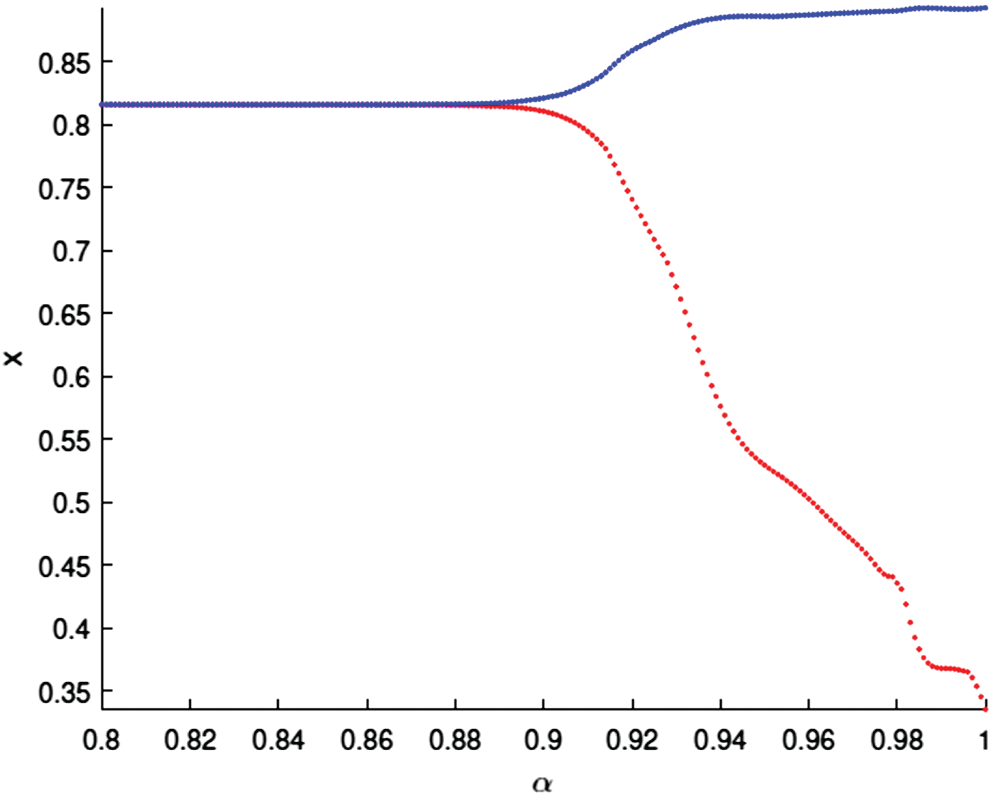
Figure 1: Bifurcation diagram of the fractional-order system (3) with respect to α
For better understand the effect of the quadratic harvesting of the middle predator
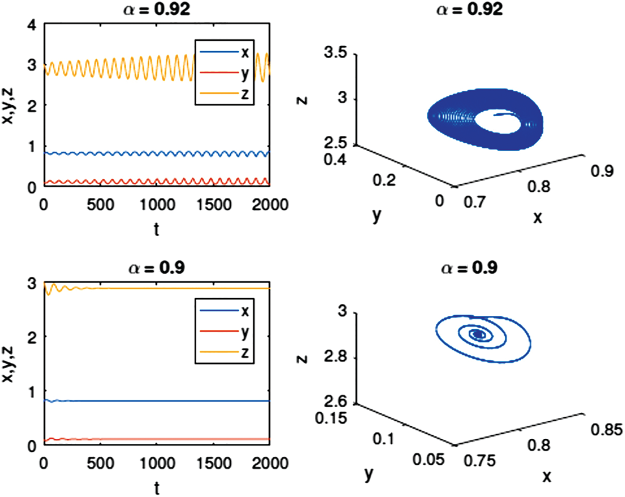
Figure 2: Time series and phase diagram of the equilibrium point E3 of model (3) with different values of α
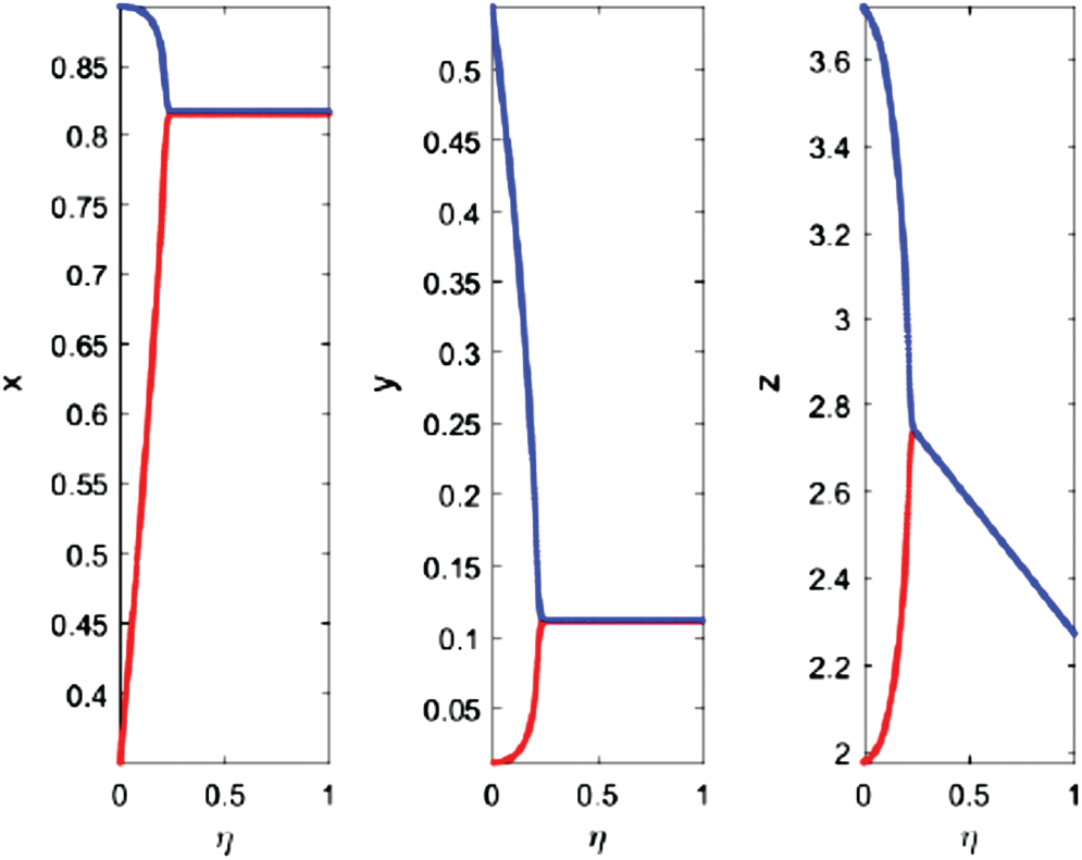
Figure 3: Bifurcation diagram of the fractional-order system (3) with respect to η
The effect of prey harvesting rate
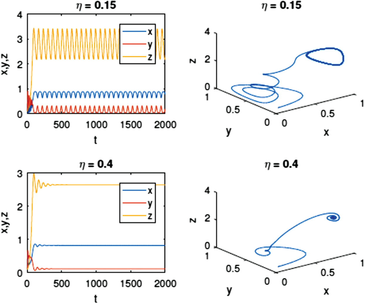
Figure 4: Time series and phase diagram of the equilibrium point E3 of model (3) with different values of η
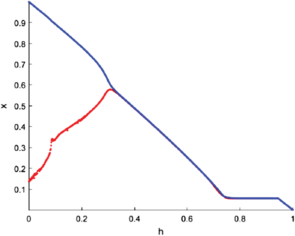
Figure 5: Bifurcation diagram of fractional-order system (3) with respect to h
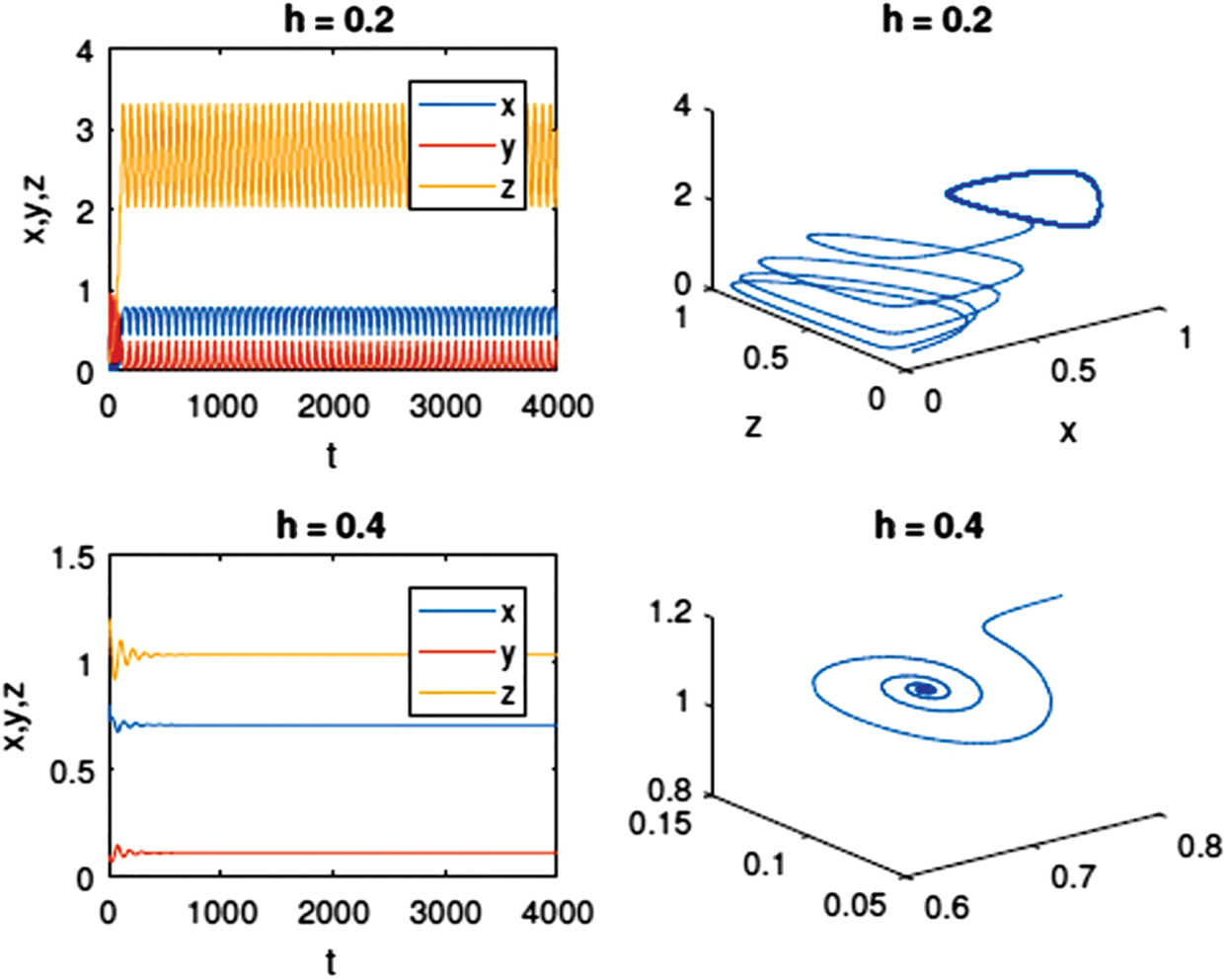
Figure 6: Time series and phase diagram of the equilibrium point E3 of model (3) with h = 0.02 and h = 0.4
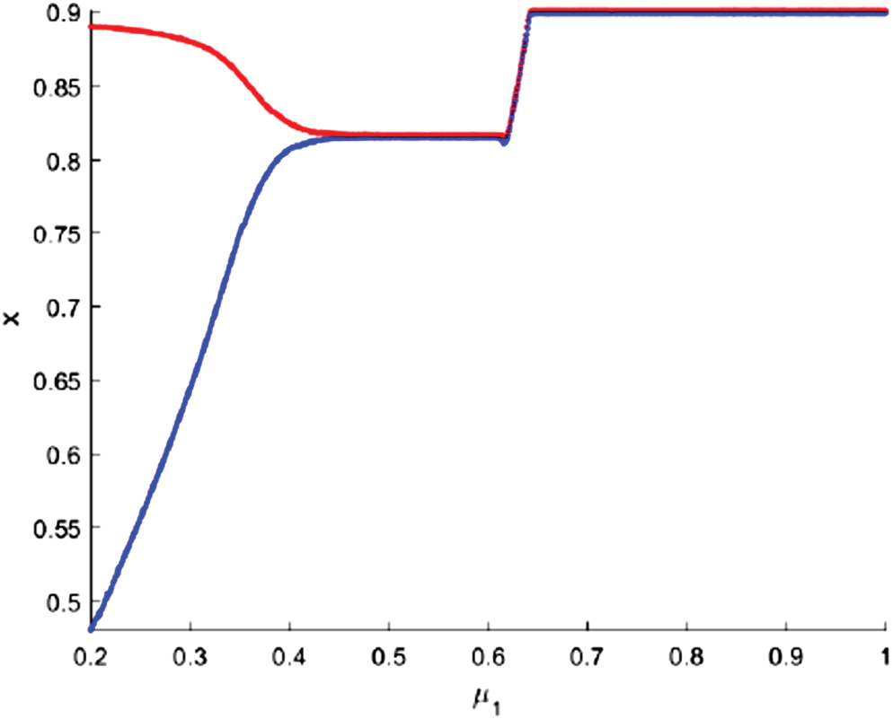
Figure 7: Bifurcation diagram of fractional-order system (3) with respect to μ1
If we increase the value of middle predator death rate
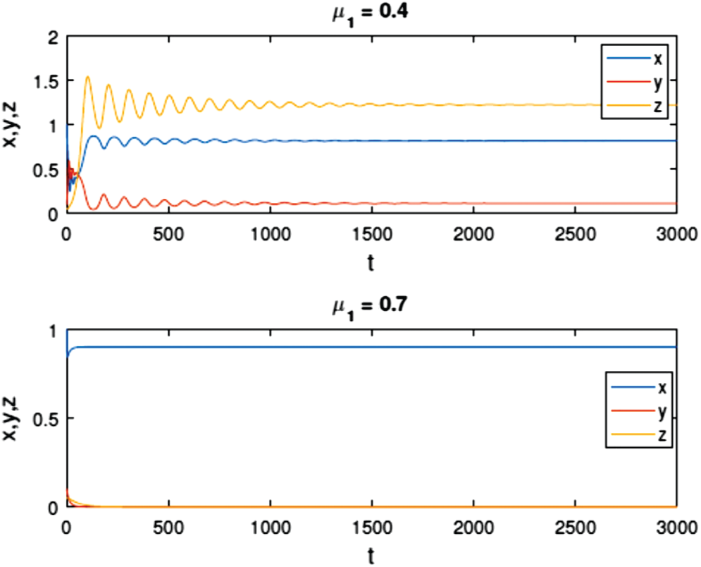
Figure 8: Time series of the food chain model (3) with μ1 = 0.4 and μ1 = 0.7
In this paper, a deterministic and stochastic fractional-order model of the tri-trophic food chain model incorporating harvesting has been proposed. It is shown that the proposed model has bounded and non-negative solution as desired in any population dynamics. By using stability analysis of fractional-order system, we have proved that if the basic reproduction number
Funding Statement: The authors gratefully acknowledge Qassim University, represented by the Deanship of Scientific Research, on the financial support under the number (cosao-bs-2019-2-2-I-5469) during the academic year 1440 AH/2019 AD.
Conflicts of Interest: The authors declare that they have no conflicts of interest to report regarding the present study.
1. A. Hastings and T. Powell, “Chaos in a three-species food chain,” Ecology, vol. 72, no. 3, pp. 896–903, 1991. [Google Scholar]
2. B. Buonomo, F. Giannino, S. Saussure and E. Venturino, “Effects of limited volatiles release by plants in tritrophic interactions,” Mathematical Biosciences and Engineering, vol. 16, no. 5, pp. 3331–3344, 2019. [Google Scholar]
3. P. Ghosh, P. Das and D. Mukherjee, “Chaos to order—Effect of random predation in a Holling type IV tri-trophic food chain system with closure terms,” International Journal of Biomathematics, vol. 9, no. 5, pp. 1650073, 2016. [Google Scholar]
4. K. Cheng, H. You and T. Yang, “Dynamics of three species food chain model with Holling type II functional response,” arXiv preprint arXiv: 2004.12237v1, 2020. [Google Scholar]
5. B. Sahoo and S. Poria, “The chaos and control of a food chain model supplying additional food to top-predator,” Chaos, Solitons & Fractals, vol. 58, pp. 52–64, 2014. [Google Scholar]
6. S. G. Mortoja, P. Panja, A. Paul, S. Bhattacharya and S. K. Mondal, “Is the intermediate predator a key regulator of a tri-trophic food chain model?: An illustration through a new functional response,” Chaos, Solitons & Fractals, vol. 132, no. 4, pp. 109613, 2020. [Google Scholar]
7. N. Pal, S. Samanta and J. Chattopadhyay, “Revisited Hastings and Powell model with omnivory and predator switching,” Chaos, Solitons & Fractals, vol. 66, no. 12, pp. 58–73, 2014. [Google Scholar]
8. N. Pal, S. Samanta and S. Rana, “The impact of constant immigration on a tri-trophic food chain model,” International Journal of Applied and Computational Mathematics, vol. 3, no. 4, pp. 3615–3644, 2017. [Google Scholar]
9. S. Raw, B. Tiwari and P. Mishra, “Analysis of a plankton-fish model with external toxicity and nonlinear harvesting,” Ricerche di Matematica, vol. 69, no. 2, pp. 653–681, 2020. [Google Scholar]
10. M. Haque, N. Ali and S. Chakravarty, “Study of a tri-trophic prey-dependent food chain model of interacting populations,” Mathematical Biosciences, vol. 246, no. 1, pp. 55–71, 2013. [Google Scholar]
11. B. Ghosh, D. Pal, T. Legovi´c and T. Kar, “Harvesting induced stability and instability in a tri-trophic food chain,” Mathematical Biosciences, vol. 304, no. 5, pp. 89–99, 2018. [Google Scholar]
12. B. Nath, N. Kumari, V. Kumar and K. P. Das, “Refugia and Allee effect in prey species stabilize chaos in a tri-trophic food chain model,” Differential Equations and Dynamical Systems, vol. 3, no. 12, pp. 591, 2019. [Google Scholar]
13. A. Matouk, A. Elsadany, E. Ahmed and H. Agiza, “Dynamical behavior of fractional-order Hastings-Powell food chain model and its discretization,” Communications in Nonlinear Science and Numerical Simulation, vol. 27, no. 1–3, pp. 153–167, 2015. [Google Scholar]
14. M. N. Huda, T. Trisilowati and A. Suryanto, “Dynamical analysis of fractional-order Hastings-Powell food chain model with alternative food,” Journal of Experimental Life Science, vol. 7, no. 1, pp. 39–44, 2017. [Google Scholar]
15. P. Panja, “Stability and dynamics of a fractional-order three-species predator-prey model,” Theory in Biosciences, vol. 138, no. 2, pp. 251–259, 2019. [Google Scholar]
16. L. Wang, H. Chang and Y. Li, “Dynamics analysis and chaotic control of a fractional-order three- species food-chain system,” Mathematics, vol. 8, no. 3, pp. 409, 2020. [Google Scholar]
17. L. Addison, “Analysis of a predator-prey model: A deterministic and stochastic approach,” J. Biom. Biostat., vol. 8, no. 4, pp. 359–368, 2017. [Google Scholar]
18. R. Ali, M. S. Arif, M. Rafiq, M. Bibi and R. Fayyaz, “Numerical analysis of stochastic vector borne plant disease model,” Computers, Materials & Continua, vol. 63, no. 1, pp. 65–83, 2020. [Google Scholar]
19. B. Ahmad, S. K. Ntouyas, A. Alsaedi and A. F. Albideewi, “A study of a coupled system of Hadamard fractional differential equations with nonlocal coupled initial-multipoint conditions,” Advances in Difference Equations, vol. 2021, no. 1, pp. 1–16, 2021. [Google Scholar]
20. S. Ahmad, R. Ullah and D. Baleanu, “Mathematical analysis of tuberculosis control model using nonsingular kernel type Caputo derivative,” Advances in Difference Equations, vol. 2021, no. 1, pp. 1–18, 2021. [Google Scholar]
21. R. Almeida, A. M. B. da Cruz, N. Martins and M. T. T. Monteiro, “An epidemiological MSEIR model described by the Caputo fractional derivative,” International Journal of Dynamics and Control, vol. 7, no. 2, pp. 776–784, 2019. [Google Scholar]
22. N. Sweilam, S. Al-Mekhlafi, A. Albalawi and D. Baleanu, “On the optimal control of coronavirus (2019-nCov) mathematical model; a numerical approach,” Advances in Difference Equations, vol. 2020, no. 1, pp. 1–13, 2020. [Google Scholar]
23. Q. Liu, D. Jiang, T. Hayat, A. Alsaedi and B. Ahmad, “Dynamical behavior of a higher order stochastically perturbed SIRI epidemic model with relapse and media coverage,” Chaos, Solitons & Fractals, vol. 139, no. Suppl. 3, pp. 110013, 2020. [Google Scholar]
24. A. I. Aliyu, M. Inc, A. Yusuf and D. Baleanu, “A fractional model of vertical transmission and cure of vector-borne diseases pertaining to the Atangana-Baleanu fractional derivatives,” Chaos, Solitons & Fractals, vol. 116, pp. 268–277, 2018. [Google Scholar]
25. I. Tejado, E. P´erez and D. Val´erio, “Fractional derivatives for economic growth modelling of the group of twenty: Application to prediction,” Mathematics, vol. 8, no. 1, pp. 50, 2020. [Google Scholar]
26. K. Shah, F. Jarad and T. Abdeljawad, “On a nonlinear fractional order model of dengue fever disease under Caputo-Fabrizio derivative,” Alexandria Engineering Journal, vol. 59, no. 4, pp. 2305–2313, 2020. [Google Scholar]
27. B. Nath and K. P. Das, “Harvesting in tri-trophic food chain stabilises the chaotic dynamics-conclusion drawn from Hastings and Powell model,” International Journal of Dynamical Systems and Differential Equations, vol. 10, no. 2, pp. 95–115, 2020. [Google Scholar]
28. J. Cresson and A. Szafran´ska, “Discrete and continuous fractional persistence problems-the positivity property and applications,” Communications in Nonlinear Science and Numerical Simulation, vol. 44, no. 3, pp. 424–448, 2017. [Google Scholar]
29. H. Li, L. Zhang, C. Hu, Y. Jiang and Z. Teng, “Dynamical analysis of a fractional-order predator- prey model incorporating a prey refuge,” Journal of Applied Mathematics and Computing, vol. 54, no. 1–2, pp. 435–449, 2017. [Google Scholar]
30. M. Sambath, P. Ramesh and K. Balachandran, “Asymptotic behavior of the fractional order three species prey-predator model,” International Journal of Nonlinear Sciences and Numerical Simulation, vol. 19, no. 7–8, pp. 721–733, 2018. [Google Scholar]
31. S. K. Choi, B. Kang and N. Koo, “Stability for Caputo fractional differential systems,” Abstract and Applied Analysis, vol. 2014, no. 3–4, pp. 1–6, 2014. [Google Scholar]
32. K. pada Das, “A mathematical study of a predator-prey dynamics with disease in predator,” International Scholarly Research Network, vol. 807486, pp. 1–16, 2011. [Google Scholar]
33. J. Huo, H. Zhao and L. Zhu, “The effect of vaccines on backward bifurcation in a fractional order HIV model,” Nonlinear Analysis: Real World Applications, vol. 26, no. 3, pp. 289–305, 2015. [Google Scholar]
34. M. S. Abdelouahab, N. E. Hamri and J. Wang, “Hopf bifurcation and chaos in fractional-order modified hybrid optical system,” Nonlinear Dynamics, vol. 69, no. 1–2, pp. 275–284, 2012. [Google Scholar]
35. L. Perko, Differential Equations and Dynamical Systems, vol. 7. New York, NY, USA: Springer, 2013. [Google Scholar]
36. W. Wang, S. Cheng, Z. Guo and X. Yan, “A note on the continuity for Caputo fractional stochastic differential equations,” Chaos: An Interdisciplinary Journal of Nonlinear Science, vol. 30, no. 7, pp. 73106, 2020. [Google Scholar]
37. T. Doan, P. Huong, P. Kloeden and A. Vu, “Euler-maruyama scheme for Caputo stochastic fractional differential equations,” Journal of Computational and Applied Mathematics, vol. 380, no. 4, pp. 112989, 2020. [Google Scholar]
38. Z. Guo, J. Hu and W. Wang, “Caratheodory’s approximation for a type of Caputo fractional stochastic differential equations,” Advances in Difference Equations, vol. 2021, no. 1, pp. 68, 2021. [Google Scholar]
39. D. T. Son, P. T. Huong, P. E. Kloeden and H. T. Tuan, “Asymptotic separation between solutions of Caputo fractional stochastic differential equations,” Stochastic Analysis and Applications, vol. 36, no. 4, pp. 654–664, 2018. [Google Scholar]
40. H. Aminikhah, A. H. R. Sheikhani, T. Houlari and H. Rezazadeh, “Numerical solution of the distributed-order fractional Bagley-Torvik equation,” IEEE/CAA Journal of Automatica Sinica, vol. 6, no. 3, pp. 760–765, 2019. [Google Scholar]
41. S. S. Ray and A. Patra, “Numerical solution of fractional stochastic neutron point kinetic equation for nuclear reactor dynamics,” Annals of Nuclear Energy, vol. 54, no. 4, pp. 154–161, 2013. [Google Scholar]
42. M. Hou, J. Yang, S. Shi and H. Liu, “Logical stochastic resonance in a nonlinear fractional-order system,” European Physical Journal Plus, vol. 135, no. 9, pp. L453, 2020. [Google Scholar]
43. G. Zou and B. Wang, “On the study of stochastic fractional-order differential equation systems,” arXiv preprint arXiv: 1611.07618, 2016. [Google Scholar]
44. I. Podlubny, Fractional Differential Equations. New York, NY, USA: Academic Press, 1999. [Google Scholar]
45. C. Huang, X. Yu, C. Wang, Z. Li and N. An, “A numerical method based on fully discrete direct discontinuous Galerkin method for the time fractional diffusion equation,” Applied Mathematics and Computation, vol. 264, no. 1, pp. 483–492, 2015. [Google Scholar]
46. C. Huang and M. Stynes, “Error analysis of a finite element method with GMMP temporal discretisation for a time-fractional diffusion equation,” Computers & Mathematics with Applications, vol. 79, no. 9, pp. 2784–2794, 2020. [Google Scholar]
 | This work is licensed under a Creative Commons Attribution 4.0 International License, which permits unrestricted use, distribution, and reproduction in any medium, provided the original work is properly cited. |