Computers, Materials & Continua DOI:10.32604/cmc.2022.019226
Article

Land-Cover Classification and its Impact on Peshawar’s Land Surface Temperature Using Remote Sensing

Shahab Ul Islam1, Saifullah Jan2, Abdul Waheed3,4,*, Gulzar Mehmood5, Mahdi Zareei6 and Faisal Alanazi7

1Department of Computer Science, IQRA National University, Peshawar, 25124, Pakistan
2Department of Computer Science, City University of Science & Information Technology, Peshawar, 25124, Pakistan
3Department of Information Technology, Hazara University, Mansehra, 21120, Pakistan
4School of Electrical and Computer Engineering, Seoul National University, Seoul, 08826, Korea
5Department of Computer Science and Information Technology, University of Malakand, 23021, Pakistan
6Tecnologico de Monterrey, School of Engineering and Sciences, Zapopan, 45201, Mexico
7Department of Electrical Engineering, Prince Sattam Bin Abdulaziz University, College of Engineering, Al Kharj, 16278, Saudi Arabia
*Corresponding Author: Abdul Waheed. Email: abdul@netlab.snu.ac.kr
Received: 07 April 2021; Accepted: 15 July 2021

Abstract: Spatial and temporal information on urban infrastructure is essential and requires various land-cover/land-use planning and management applications. Besides, a change in infrastructure has a direct impact on other land-cover and climatic conditions. This study assessed changes in the rate and spatial distribution of Peshawar district’s infrastructure and its effects on Land Surface Temperature (LST) during the years 1996 and 2019. For this purpose, firstly, satellite images of bands7 and 8 ETM+(Enhanced Thematic Mapper) plus and OLI (Operational Land Imager) of 30 m resolution were taken. Secondly, for classification and image processing, remote sensing (RS) applications ENVI (Environment for Visualising Images) and GIS (Geographic Information System) were used. Thirdly, for better visualization and more in-depth analysis of land sat images, pre-processing techniques were employed. For Land use and Land cover (LU/LC) four types of land cover areas were identified – vegetation area, water cover, urbanized area, and infertile land for the years under research. The composition of red, green, and near infra-red bands was used for supervised classification. Classified images were extracted for analyzing the relative infrastructure change. A comparative analysis for the classification of images is performed for SVM (Support Vector Machine) and ANN (Artificial Neural Network). Based on analyzing these images, the result shows the rise in the average temperature from 30.04°C to 45.25°C. This only possible reason is the increase in the built-up area from 78.73 to 332.78 Area km2 from 1996 to 2019. It has also been witnessed that the city’s sides are hotter than the city’s center due to the barren land on the borders.

Keywords: Remote sensing; temperature extraction; urbanization; satellite image classification; artificial neural network; support vector machine; LU/LC; land surface temperature

1  Introduction

Remote sensing is the science of getting information without any physical contact about the earth or an object on the earth [1]. The essential research goal in remote sensing is using satellite data for the LU/LC classification. The leading cause of global warming is the forests degradation, deforestation, and urbanization. The satellite data for LU/LC information nowadays is essential for global environmental protection [2]. The RS (Remote Sensing) community implements the LU/LC system for mapping the features of the earth’s surface. LU/LC indicates that how much area is covered by a different type of land and how this landscape is using by the people [3]. Getting the most reliable and adequate information about the landscape LU/LC classification is one of the most important applications of remote sensing. In remote sensing, to extract useful information from satellite data, several classifiers are used. In this work, the LU/LC classification has been done for the Peshawar test patch using Artificial Neural Network (ANN) and Support Vector Machine (SVM) supervised classifiers. Besides the LU/LC classification, temperature extraction has also been done in this work. Many factors contribute to causing global warming and climate change, but the temperature is one of the main factors. A continuous rise may found in the annual temperature worldwide in the past 150 years. The LU/LC change of a city also changes the LST profiles of a city. Different land surface with different emissivity has different temperature [4]. LU/LC change in the present work has a remarkable contribution to changing the urban and local temperature.

1.1 Urbanization

Human populations increase over time, which leads people to live in groups and communities. According to the development in those communities, some came to be recognized as rural settlements, while those with more progress were called the cities. The development process in the urban areas led more people to settle in those areas. This process is known as urbanization. This urbanization resulted in rapid population growth in the cities [5]. However, during this urbanization, a large number of people still lived and worked in rural settlements. It was the eighteen-century industrial revolution that attracted a large scale population towards urban areas. Approximately the world’s half population is moving towards cities. Since these areas provide comparatively more employment, better education, and increase recreation facilities. During industrialization, many countries experience this urbanization; nonetheless, those previously industrialized nations have already been through this process of urbanization. Thus, urbanization is a global phenomenon and as with other phenomena, urbanization also entails some severe disadvantages [6]. The creation of megacities is one of the essential aspects of urbanization. Megacities are cities with more than ten million populations. This, however, has now changed to cities with even double than ten million; for instance, the Japanese city Tokyo has a population of forty million. This has resulted in urban sprawl, which increases the city’s geographical area because of its population growth. In this process, the cities take up the areas which were formerly used for agricultural purposes. These suburbs of the cities now serve residential and industrial functions [7]. This sprawl calls for infrastructural development, especially for transportation, since people are likely to live far from the workplace and need daily commuting to and from one end of the city to another. LU/LC change related to urbanization produces consequences such as a rise in temperature and low air quality [8]. The population will continually grow in urban areas and their population. This will lead to further complex challenges of urbanization in the future. Planning to deal with the likely effects of this urbanization will have consequences for our world in the future.

1.2 Land Surface Temperature

Many factors contribute to causing global warming and climate change, but temperature is one of the main factors. A continuous rise may be found in the annual temperature worldwide in the past 150 years. The LU/LC change of a city also changes the land surface temperature (LST) profile of a city. Different land surface with different emissivity has different temperature [9,10]. LU/LC change in the present work has a remarkable contribution to changing the urban and local temperature. It has a substantial impact on the natural rounds of the atmosphere. By the year 2050, it is anticipated that more than half of the world’s population will move towards urban areas [11]. An obvious picture of the land surface and the climate’s physical properties can be declared by the LST, which is involved in the environment’s several processes. Measuring the air temperature by using temperature sensors is expensive and time-consuming as it requires the building of temperature sensors at the preferred places in the city.

1.3 Remote Sensing

Remote sensing is acquiring details about an object without any physical interaction with that object. Satellite sensors obtain this information about the object. Farmers can use remote sensing to observe their fields without physically visiting the area continuously. The farmers can monitor the overall image of their plantations, extracted through different classification tools. These satellite images give the farmers essential information to plan better for their fields [12,13]. The function of remote sensing is to provide data that helps analyze the variabilities of temporal and spatial parameters of the environment on a large scale. This data is utilized for crop yield appraisal, growth regulations, environmental damage evaluation, land-use monitoring, calculations, surrounding explorations, town planning, radiation monitoring, and geographical maps for civil and military purposes. Remote sensing’s most essential function is to classify and map the land cover aspects such as vegetation, soil, water bodies, and forests [14]. The Remote Sensing study includes photography, computer systems, spectroscopy, electronics satellite propelling, optical communication and media studies, etc. Remote sensing integrates these innovations in one complete system. The remote sensing process is achieved through several stages essential to its successful operation, as shown in Fig. 1.

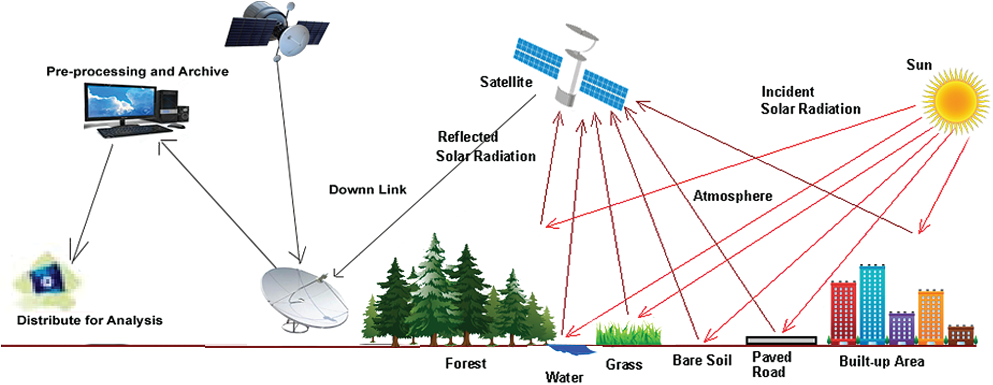
Figure 1: Remote sensing process

Two main types of remote sensing are Passive and Active remote sensing. Passive sensors are used in passive remote sensing. These sensors utilize light to capture the image. These sensors are installed on satellites, aircraft, or drones; these sensors detect the natural radiation reflected from the objects or the earth’s area. Radiometers, infrared, and photography are some other examples of passive remote sensors. Fig. 2 shows the passive remote sensing process.

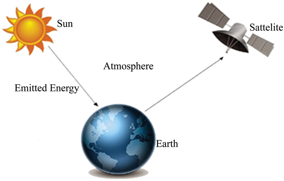
Figure 2: Passive remote sensing

Active remote sensing uses active sensors, which respond to internal stimuli of objects. It records an object’s vitality. The energy is sent to objects or territories, sensors distinguish and the radiation is measured that reflects from objects. Examples of active remote sensing are LIDAR and RADAR [15]. Fig. 3 shows the active remote sensing process.

1.4 Image Classification

Image classification is the most significant field in processing research, particularly in pattern recognition. Image classification is a significant objective for ecological applications. Image pixels in classification can be characterized either by division/segmentation or by factual belongings of multivariable dependent on both spatial and measurable associations with adjoining pixels [16].

1.5 Paper Contribution

About urbanization, especially for climate systems, temperature is the most key parameter. The main objectives of the current study were;

1.    The LU/LC classification of Peshawar region using supervised classifiers, i.e., artificial neural network (ANN) and support vector machine (SVM).

2.    To compare the overall accuracies of these supervised classifiers to evaluate the performance.

3.    Land Surface Temperature retrieval during 1996 and 2019.

4.    To assess spatiotemporal changes in the LU/LC and LST and develop a relationship between LU/LC classes and LST. The Peshawar region has been chosen as a study area in the current work. For analysis, the imagery data of the last 22 years (1996–2019) were obtained from the United States Geological Survey (USGS) earth explorer site and SUPARCO (Space and Upper Atmosphere Research Commission) Pakistan. For city planning to reduce the city temperature, it will help communicate the green cover LU/LC classification guidelines.

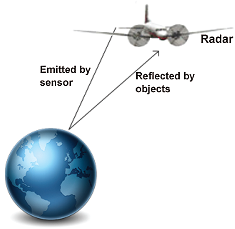
Figure 3: Active remote sensing

1.6 Paper Organization

The proposed work comprises of 7 sections: In Section 2, the literature review has been discussed, Section 3 presents the materials and methods, the methodology has been discussed in Section 4 and Section 5 consists of the experiments and results which demonstrate the simulation results using ENVI & GIS tool, in Section 6 we compare our work with the previous studies and Section 7 presents the conclusion.

2  Literature Review

For LU/LC classification and LST retrieval, different approaches and steps have been followed in this section. Work done on LU/LC classification and LST is reviewed in this section. Mukherje et al. [17] Researched LU/LC and LST variations in India by comparing the two urban areas. They studied LC/LU and LST’s effect on vegetation and water resources for 29 years, i.e., 1988 to 2017. Results showed that sugarcane and rice were less unstable than cotton and wheat. Their study included LU/LC and LST impact on water bodies and agriculture from 1988 to 2017. The LU/LC found that sugarcane and rice crops were less volatile than wheat and cotton crops. For understanding the LC/LU results, both user’s and producer’s accuracy is essential. The producer’s accuracy is considered the map accuracy of the map’s creator, while the accuracy of the user is defined as the accuracy of the person using the map. Their research showed 85.7% for winter crops and 87.7% for summer crops in the general user’s and producer’s accuracy. The study also revealed that from 1988 to 2017, urban development increased by 7.2% in all classes in the district Multan. Increased urban development has caused a gradual decrease in farming activities, ultimately giving rise to land surface temperature. The study proved that LU/LC changes and LST from 1988 to 2017 brought drastic changes in vegetation patterns and increased temperature in the Multan district. Talukdar et al. [18] conducted the study to investigate the accuracy of various machine learning classifiers for LU/LC classifications. The main goal of this study was to suggest the best LU/LC classifier. The authors applied various machine learning algorithms on Landsat 08 (OLI) data for classification. The result shows that area varies different classifiers under each LU/LC class. The maximum changes were noted for the agricultural land and the minimum for the water bodies. Such variations require the best-suited classifier to be proved. This work concludes that in the highly dynamic charland-dominated areas RF is the best machine-learning classifier for LULC modeling. Straub et al. [19] studied the inconsistency of LU/LC variations of Spatiotemporal and its association with LST. The results were linked with the Indian and Bangladesh parts. Their approach tendency was examined in cities with more than 1 million populations and towns with more than 100,000 populations. Changes in Land Surface Temperature were mainly determined by LU/LC changes along both countries’ borders. The leading form of LU/LC change is urbanization. Compared to the period from 1989 to 2005, the rate at which land changed from 2005 to 2010 is much faster. 1.83°C decrease in LST at Indian part and 1.85°C in the Bangladesh part was observed over 21 years. The decline in LST was observed in areas that converged from rural to agricultural, while an increase in LST increased in those joined to urban. LU/LC and LST relationships are high in large cities like Kolkata and Khulna. This research’s results are significant for monitoring LU/LC changes in spatial decision support system development. This research serves as a baseline to examine the impact of LU/LC changes in the mentioned study area. Likewise, Khan et al. [20] studied the pattern of LU/LC, Normalized Difference Vegetation Index, and Normalized Difference Built-up Index variations in district Lodhran, Pakistan. They studied four major types of LU/LC Land sat images from 1977 to 2017. These four LU/LC types are vegetation cover, built-up areas, soil and water cover. These researchers used supervised classification, i.e., the maximum likelihood for detecting LU/LC changes in district Lodhran using ERDAS software. Imagine 15.46.6% of farmers observed a great change in temperature, plantation season, and reduced rainfall in the past few years in Lodhran district. From the year 1977 to 2017, urban areas increased by 4.3%. Normalized Difference Vegetation Index variations values were high in 1977(+0.86) and low in 1997(0.33). Classification overall accuracy for the years 1977, 1987, 1997, 2007 and 2017 were 86%, 85%, 86%, 88%, 95% respectively. NDVI, LU/LC change with soil, temperature, NDBI, and slope classes were common in the study area. In the past 40 years, the plain soil’s alteration to agriculture and urban areas was the major variation in the study area. Less irrigation water resources, downflow in rainfall, and temperature rise were the challenges Lodhran district faces. Local farmers were adopting different strategies to overcome the effects of these climatic changes, but they need support from government agencies. Liaqut et al. [21] examined the changes in LU/LC of the Asansol-Durgapur Region by using multi-temporal satellite data. The study uses 4–5 TM and LANDSAT 8 OLI data of 1993, 2009, and 2015. Land Surface Temperatures of winter, summer and post-monsoon periods are studied in this research. The study finds that radiant surface temperature is dependent upon various LU/LC units. The research found increased surface temperature, i.e., 38°C over coal mines, industries, and hardcore surfaces, while 27°C was observed over water surfaces and green areas. For classifying the satellite image, Choudhury et al. [22] Reviewed different ANN approaches. Every classification needs another classification time to classify satellite images. The reason for different times is algorithm dependency on several classes and training samples. They compared the accuracies of different classifying techniques with ANN. Their experiments showed some excellent techniques to classify LU/LC maps for weather forecasting, archaeology, deforestation, damage assessment, and development. According to Mohamed et al. [23], categorizing and extracting essential information regarding LU/LC is done through remote sensing. This data is utilized in planning for the built-up area, ecological growth of the environment, and sustainable urban monitoring. Therefore, remote sensing is helping researchers use this technology in ecologically sound geographical planning of our earth. To investigate the spatial variations in the different urbanized areas on urban renewal and LST, Hou et al. [24] have worked on the center and borders regions in Fuzhou City, China, between 2007 and 2017. The authors stated that the urban renewal process helps drop in LST in core region districts with relatively high urbanization. In contrast, the side areas with relatively low urbanization presented the opposite characteristics. The result can be explained by combining building density, population density, and landscape pattern variations in urban renewal. The authors further stated that to promote greater awareness of this issue in management practices and future planning, our study’s results provide a new perspective on urban renewal’s impact on thermal environmental and urban microclimates changes.

3  Materials and Methods

This section discusses the main area of study and imagery data that which type of satellite data has been collected for LU/LC classification and further temperature extraction.

3.1 Study Area

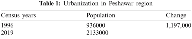
District Peshawar, 340 m above sea level and 1257 km2, is located at 34°0′28.8″ N 71°34′42.6″ E in Khyber Pakhtunkhwa province. On three sides, the valley of Peshawar was surrounded by mountain ranges, with the fourth opening to Punjab province shown in Fig. 4. The oldest history dates back to 539 BCE, making Peshawar one of the oldest cities in Pakistan and throughout the world [20]. The sixth-largest city of Pakistan is Peshawar, according to the 2019 census, with a population of 2,133,000 (Tab. 1) (Pakistan Bureau of Statistics, 2019). According to the Koppen classification, Peshawar has a hot semi-arid climate, with mild winters and sizzling summers.

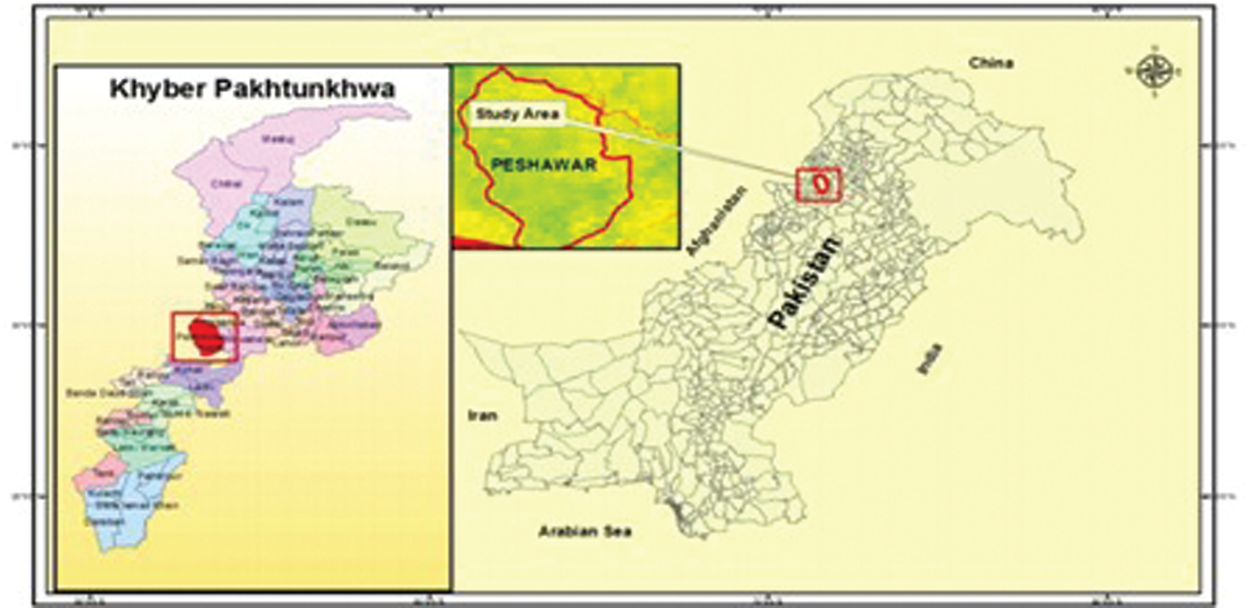
Figure 4: Map of peshawar region (The study area)

3.2 Imagery Data

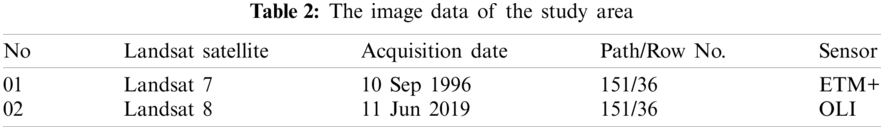
The free and open data sets (multispectral and multi-temporal Landsat satellite imagery) were collected from USGS (United States Geological Survey) and SUPARCO (Space and Upper Atmosphere Research Commission). The analysis was based on the two data sets, i.e., 1996 and 2019. According to the NLCD, the land cover classification has four main types, i.e., water bodies, agricultural land, settlements, and barren land. This land-use data were imitated from the 30-m resolution Landsat ETM+/OLI images. Tab. 2 shows the imagery data that were downloaded based on the satellite availability for the Peshawar region. The Peshawar region’s paths 151 and row are 36, which becomes 151/36, as shown in Tab. 2. By putting the raster form of the imagery data in GIS, the ROI was separated from the rest of the image using the subset image tool.

4  Methodology

The Landsat ETM+ and OLI images were obtained and carried out data pre-processing, as shown in Fig. 5. The median filter was applied to the pre-processed data. After this, we selected the ROIs as training samples for LU/LC classification. The accuracy assessment took place after the classification. After the radiometric correction, the digital number was converted to spectral radiance. Then NDVI and land surface emissivity were calculated. After that, the Land surface temperature has been calculated from Landsat imagery. Once the LST has been obtained, the LST urbanization impact has been evaluated and the LU/LC is correlated with the LST.

4.1 Pre Processing

Pre-processing is the first step of classification and is carried out to remove noise from the image. For the proposed set-up, a reduction in atmospheric correction, fog, and band ratio discovery is made in the pre-processing phase. Fig. 6 shows the workflow of image pre-processing.

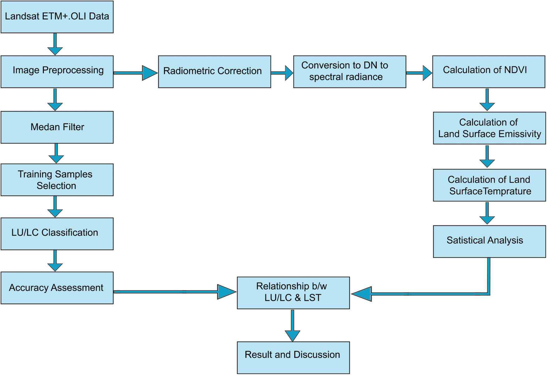
Figure 5: Workflow for LU/LC classification and investigating the impact of urbanization on land surface temperature (LST), based on the combination of ETM+/OLI images

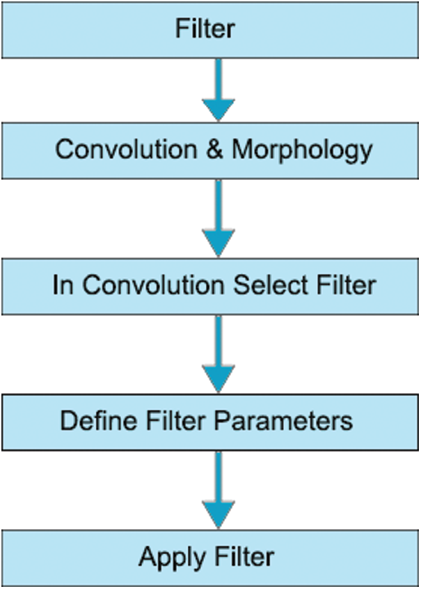
Figure 6: Image processing work flow

4.2 Convolution and Morphology

To remove noise and fog from images, another filter by the name of “convolution and morphology” is applied to the image. The objective of this filter is the evaluation of geometrical structures. For this filter, the relative ordering of pixels is essential rather than the pixels’ numerical value. Morphological filtering effectively works on digital images. Convolution and Morphology filter is available in ENVI 4.7 tool under the heading of filter tab. Click on the Filter tab in the menu and then on Convolution and Morphology. Figs. 7 and 8 show the convolution morphology tool and processing.

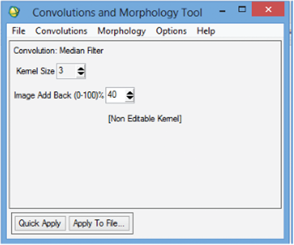
Figure 7: Convolution morphology tool

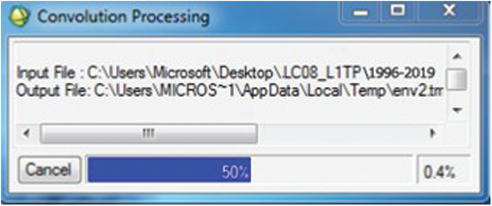
Figure 8: Convolution process

4.3 Median Filter

The median filter is applied to make the image smooth while conserving edges more significant than kernel dimensions. The central pixel value is replaced with the median value. Removing speckling noise from the image, the median filter produces better results. Fig. 9 shows the filtered image after the pre-processing and applying median filter. To sharpen an image, the median filter is provided by the Add Back value. To preserve an image’s spatial context, the Add Back value adds the original image’s back. Add back value is the percentage of the original image included in the final image output. If the Add Back value is 40%, at that point, 40% of the actual image is added to 60% of the final production. Add Back values, added to the median filter, are shown in Fig. 7. Click on Quick Apply or Apply button to add this data to the convolution and morphology tool. The input data is given to the C&M tool; the median filter is then used to acquire the desired filtered patch. A band list will appear once the convolution process is completed and we have to select the grayscale and RBG bands.

Figure 9: Filtered image

4.4 Training Sample

Selecting training samples is the second step of image classification. This sample is used for the automatic classification of a particular data set. This training sample is needed for each class and the number of required classes depends on research interest.

4.5 Region of Interest

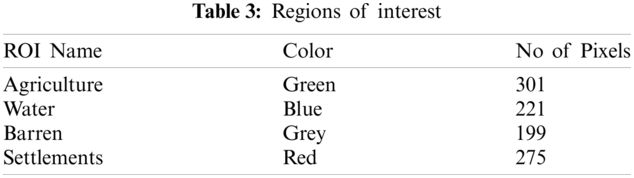
Region of Interest (ROI) are subsets of sample data. Region of Interest is selected as a polygon. ROI defines the border of an object under observation. Once the filtered image is opened, click on tools and then the region of interest. A dialogue box will pop up, showing ROI tools. Select the desired area by drawing a polygon. Several pixels selected will be highlighted as a sample shown in Fig. 10. The number of pixels and colors for the LU/LC classes are mentioned below in Tab. 3.

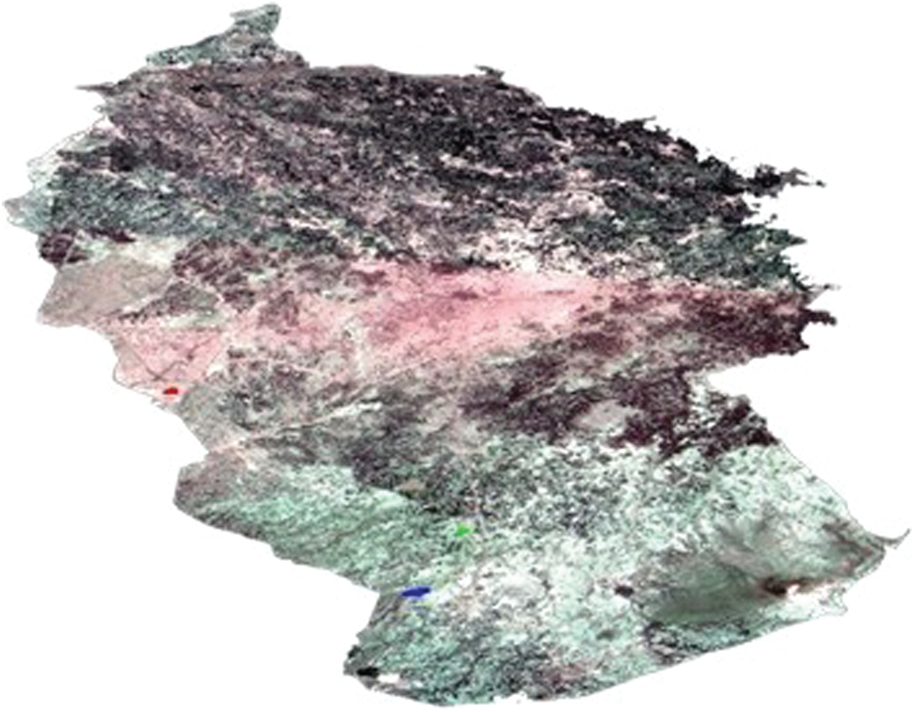
Figure 10: Selection of different classes as ROI

4.6 Decision

The decision step of image classification is based on the training sample where the system is tested for a decision. For comparison of image pattern with the desired image, we select the appropriate procedure. Once the sample is taken, image classification is carried out using a supervised classification algorithm.

4.7 Image and the Supervised Classifications

There are different bands with combined features in unclassified images that cannot be distinguished. To turn these images into their features, supervised classifiers can be used [25], i.e., agriculture, barren land, water bodies, and urban area. Different band combinations were used to view the image to classify the various features. LU/LC classification can be achieved by classifying the satellite images. For each class, simple has been taken in polygon form with pixels mentioned in Tab. 3. Two supervised classifiers Artificial-Neural- Network (ANN) and Support-Vector-Machine (SVM), were used after testing. The classification algorithm is selected once the training sample is added. ANN and SVM are selected by clicking the classification menu and then supervised classification.

4.7.1 Artificial Neural Network (ANN)

Neural Net is selected from the menu, which then asks about the file to be classified. A pre-processed filtered image is added as the input file. Tap the OK button once the file is added for classification, resulting in a dialogue box showing Neural Net parameters. Select the number of classes and set parameters for ANN. Provide a path for the output file and click the OK button. Once all the parameters are set, Tap the OK button, the classification will start. A progress bar pop-up will notify the start of classification. RMS error will be shown at each iteration. The lower value of RMS error shows the training is done correctly. Available Band List will appear as soon as the classification ends. RGB mode is selected. Based on ROI, the output image is generated by the ANN classifier. Color representation is as follows:

4.7.2 Support Vector Machine (SVM)

Click on classification in the menu tab, then supervised classification, and then Support Vector Machine. A new window will pop up, asking for opening a file for classification. The filtered file is selected and is given to SVM as an input file. By tapping on the OK button, another window of Support Vector Machine Classification will spring up. Output depends upon parameters set in SVM. Once the classification is completed, Available Band List options will be shown on the desktop. RGB mode is selected and Load RGB is clicked to generate the output image based on ROI.

5  Experimentation & Results

Land use is the classification of natural environments and their resources into built-up like settlements etc. In contrast, land cover encompasses the physical state of the earth’s surface. The land cover classes in the images may vary significantly, depending upon the type and number of the classes and sensor resolution. The LU/LC classification was analyzed using remote sensing techniques using ENVI 4.7 and the GIS tool in this work. Remote sensing and GIS technology together provide unique and most important information about LU/LC classification [26]. Fig. 11 shows the LU/LC classification of 1996 and 2019 imagery data using ANN. The study area’s imagery data were classified into four classes, i.e., settlements, agriculture, barren land, and water bodies. 1257 km2 was the total classified area. The kappa coefficient and overall accuracy of ANN are mentioned in Tab. 4.

5.1 Estimation of NDVI

Visible and near-infrared electromagnetic spectrum bands are used to calculate the Normalized Difference Vegetation Index NDVI is the best tool to observe the presence of vegetation areas and their strength. The general Eq. (1) for deriving NDVI values is shown in Tab. 3:

NDVI=(NIR−RED)/(NIR+RED) (1)

The value of the NDVI index is between 1 and 1.

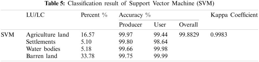
Fig. 12 shows the LU/LC classification of 1996 and 2019 imagery data using SVM. The study area’s imagery data were also classified into four classes, i.e., settlements, agriculture, barren land, and water bodies. 1257 km2 was the total classified area. The kappa coefficient and overall accuracy of SVM are mentioned in Tab. 5.

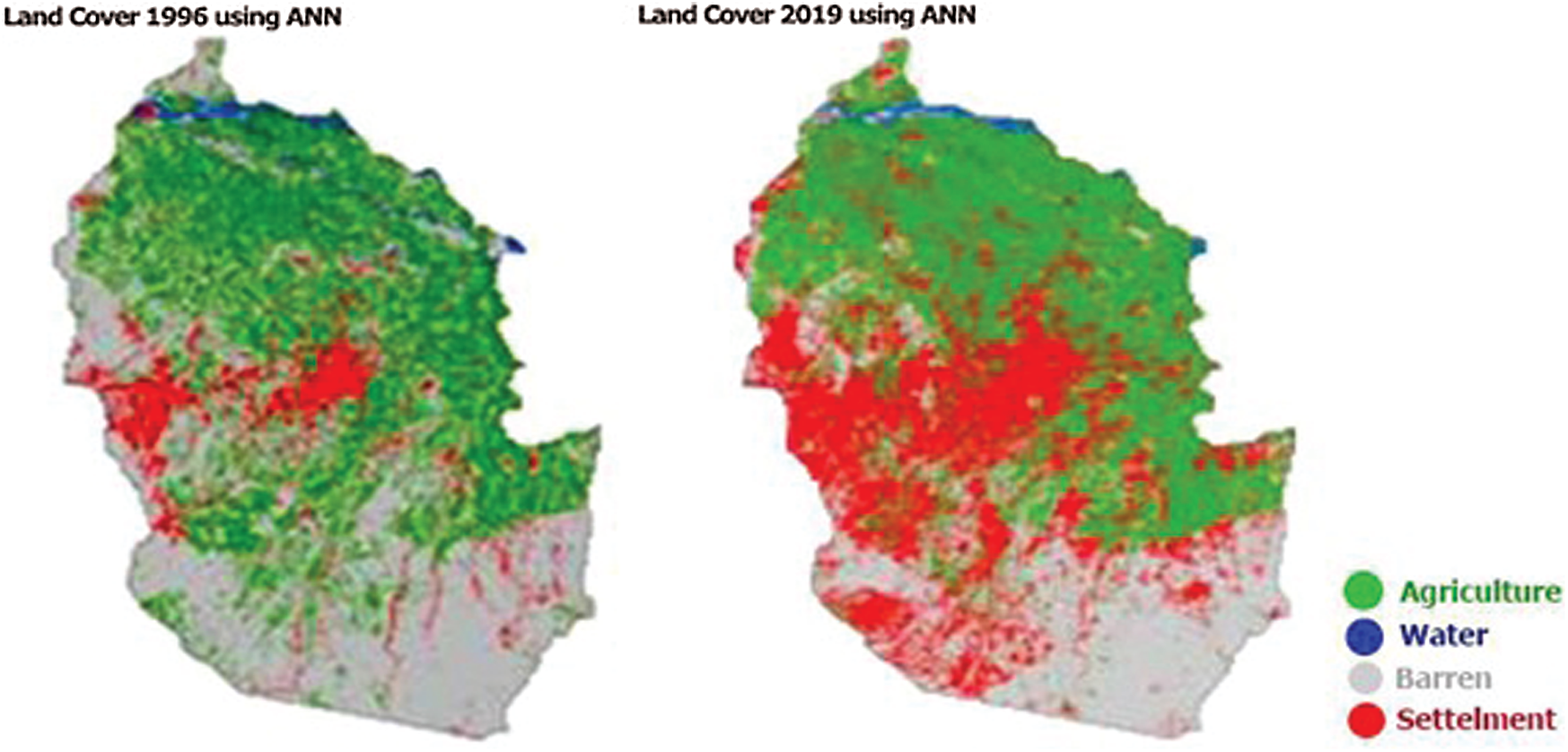
Figure 11: The land cover result of Artificial Neural Network (ANN)

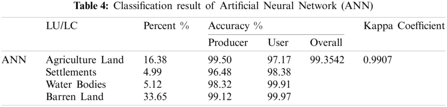
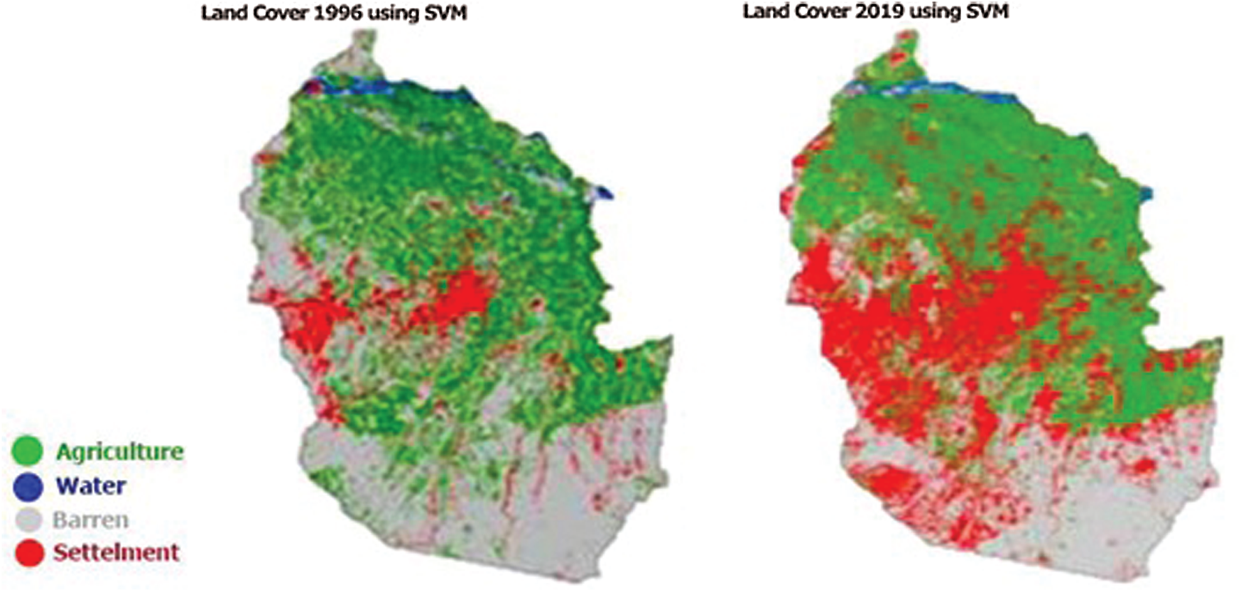
Figure 12: The land cover result of Support Vector Machine (SVM)

5.2 Accuracy of Classification

Assessing the classification accuracy is the last step in supervised classification and is carried out after completing the classification phase. LU/LC maps will be produced with accuracy by using a confusion matrix. The LU/LC classification output of the ANN and SVM are shown in Tab. 6. The table shows the overall accuracy obtained from the post-classification in the confusion matrix: the user and producer accuracy and the kappa coefficient calculated using Eq. (2).

K=N∑i=1nmi,i−∑i=1n(GiCi)N2−∑i=1n(GiCi) (2)

where :

•   i is the number of classes.

•   N is the total number of classified values compared to truth values.

•   mi,i is the number of values belonging to the truth class i that have also been classified as class i (i.e., values found along the diagonal of the confusion matrix).

•   Ci is the total number of predicted values belonging to class i.

•   Gi is the total number of truth values belonging to class i.

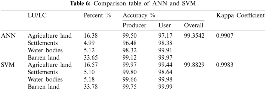
Agriculture, Settlements, Water Bodies, and Barren land have an overall high accuracy in SVM. The table shows that ANN has an overall accuracy of 99.3542% and the Kappa coefficient of 0.9907, while the overall accuracy obtained from SVM is 99.8829%, and the Kappa coefficient of 0.9983. So the overall accuracy indicates that SVM is the highest in declaring higher accuracy for LU/LC classification. A comparative analysis of the Artificial Neural Network and Support Vector Machine state has been summarized in Tab. 6.

5.3 Land Surface Temperature Retrieval

5.3.1 Estimation of LST

How hot the earth's surface would feel touching in a particular region is Land Surface Temperature. Thematic Mapper, Enhanced Thematic Mapper, and thermal bands having spatial resolutions are used to calculate LST. For the estimation of land surface temperature, the digital number needs to be converted as spectral radiance: Eq. (3) is used to change the digital number to spectral radiance.

Lλ=gain∗DN+offset (3)

Eq. (4) is used to convert the spectral radiance to temperature.

T=K2/ln⁡(K1/Lλ+1) (4)

This temperature is in Kelvin scale, which is then converted to Celsius scale by the Eq. (5)

T(C∘)=T(K)−273.15 (5)

The T is the temperature in degree Kelvin and i is the land surface’s emissivity value. The angular effects and spectral emissivity values at the surface, atmospheric attenuation, and viz, these effects need to be corrected to convert radiances to the LST [27]. The study measures the city’s urbanization on climate, not generating the parameters for climatological modeling. In the current work, spectral emissivity at the surface is considered to develop a cause-effect relationship between development activity and LST increase.

5.3.2 Urbanization Effect on Land Surface Temperature

NDVI and LST reflect the impact of urbanization on the study area. Industrialization, settlement, decreases in vegetation areas and different economic activities increase ground surface temperature [28]. The negative correlation between NDVI and LST is found in the study. An increase in surface temperature is observed in fewer vegetation areas. Buildings, surface soil nature, and settlement in the central part of the site under study directly impact surface temperature. The land surface temperature obtains through satellite imagery. Maximum 35.4°C and 15.6°C minimum were observed inland sat ETM+ 2000, with a mean value of 25.5°C. For 2019 Land sat OLI/TIRS, maximum temperature value 43.5°C and minimum 21.9°C, with a mean value of 32.7°C. According to the infrastructure, the research area’s core portion showed high temperature and is considered more developed than the borders area. Figs. 13 and 14 show the Peshawar region’s land surface temperature during 1996 and 2019, respectively.

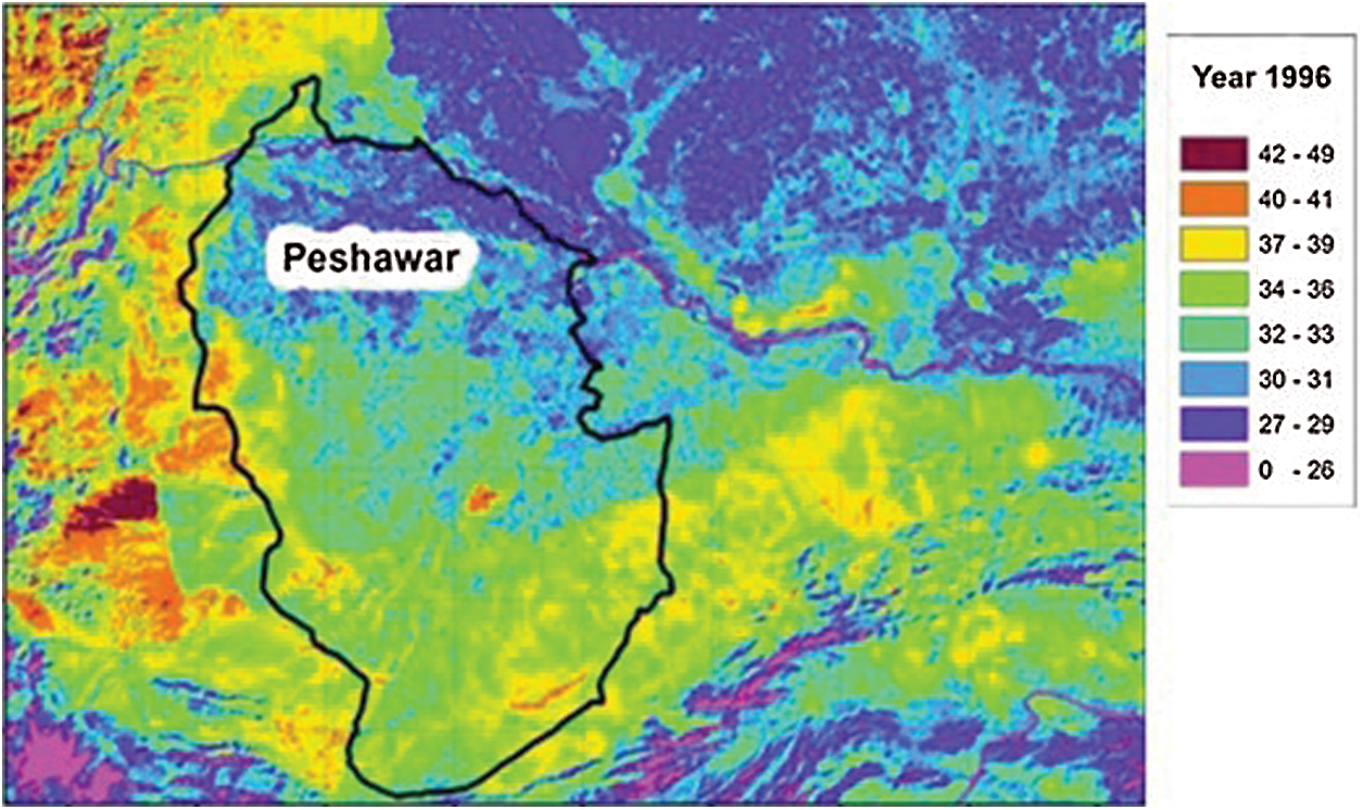
Figure 13: Land surface temperature of Peshawar during 1996

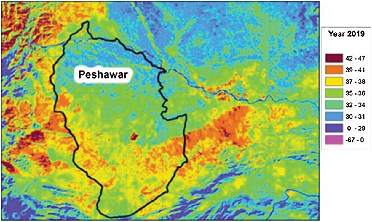
Figure 14: Land surface temperature of Peshawar during 2019

5.3.3 Relationship Between LST and LU/LC

The class-wise LST was pared from the original classified image to induce the relationship between the LST and various LU/LC classes and the statistics of the same were determined. To determine the relationship between mean LST and LU/LC classes, this was done for both of the images and the scatterplot was generated. Figs. 15 and 16 show the relationship between LU/LC and LST during 1996 and 2019.

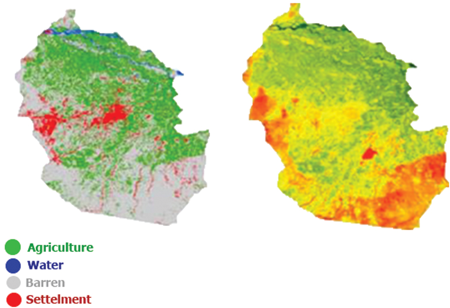
Figure 15: Land cover & surface temperature of 1996 data

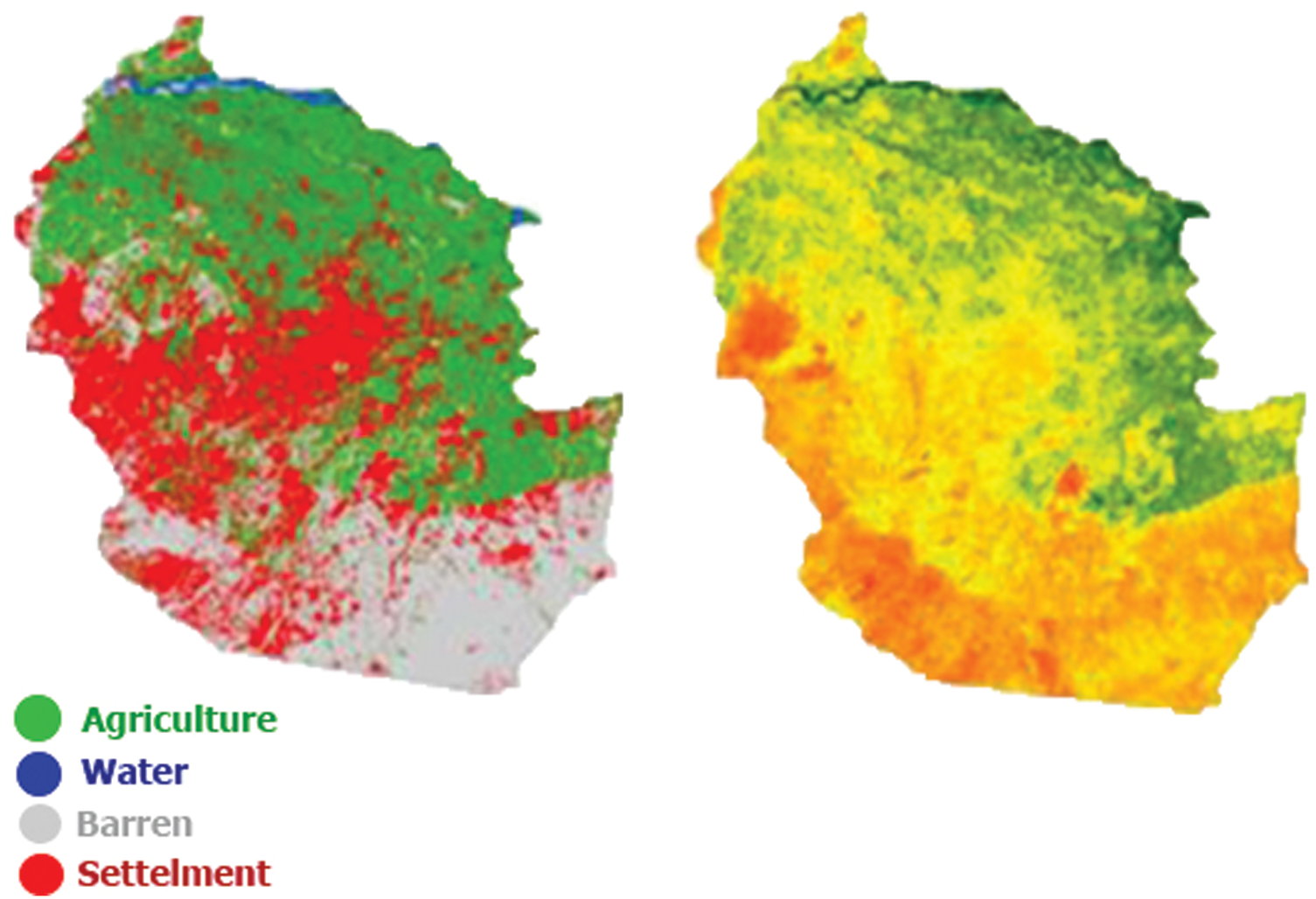
Figure 16: Land cover & surface temperature of 2019 data

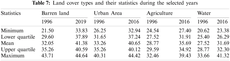
LST of the various land cover classes during 1996 and 2019 are shown in Fig. 17. Tab. 7 shows the land-use change during 1996 and 2019. The findings discovered that the barren land shows a decreasing trend in these two phases, while the urban area portrays the increasing trend over time in our study area. The maximum, mean and minimum temperature of the various land cover classes in the lower and upper quartile shows that a substantial LST difference exists over land cover classes. The mean surface temperature of the barren land was 32.05°C and 41.38°C during 1996 and 2019 respectively shown in Fig. 17. The urban area’s mean surface temperature was 33.26°C and 40.65°C during 1996 and 2019. Similarly, the mean surface temperature of the agricultural land was 28.77°C and 35.69°C during 1996 and 2019 respectively, while the mean temperature of water bodies was 27.52°C and 31.69°C during the same period, respectively. The growing trend in the LST and climate change has led to a global effort to invent specific policies for sustainable energy sources, less energy-intensive economic development, and sustainable agriculture. The overall result showed that the water bodies and agricultural land have a low temperature than the urban and barren land, which has a high surface temperature. There are various factors such as land-use change, land surface parameters, economic development, seasonal variation, and population growth, which affect the land surface temperature [29]. There is a clear difference between the two imageries in terms of temperatures, as shown in Figs. 15 and 16. Urban heat islands are created due to urbanization and human industrial activities. The figure shows that the barren and urban areas have the maximum, while water and agricultural land hold minimum Land surface temperature during 1996 and 2019. Further, the land surface temperature of barren land is higher than in an urban area. The only reason for this is that urban land is covered by green land. This research illustrates that the urban area’s temperature increases from 30.04°C to 45.25°C and the average temperature of the barren land increases from 34.06°C to 42.07°C during 1996–2019. Simultaneously, the average temperature of agricultural land rises by 10°C and 5.89°C during 1996–2019, respectively. This leads to the conclusion that the surface temperature is increased as time passes.

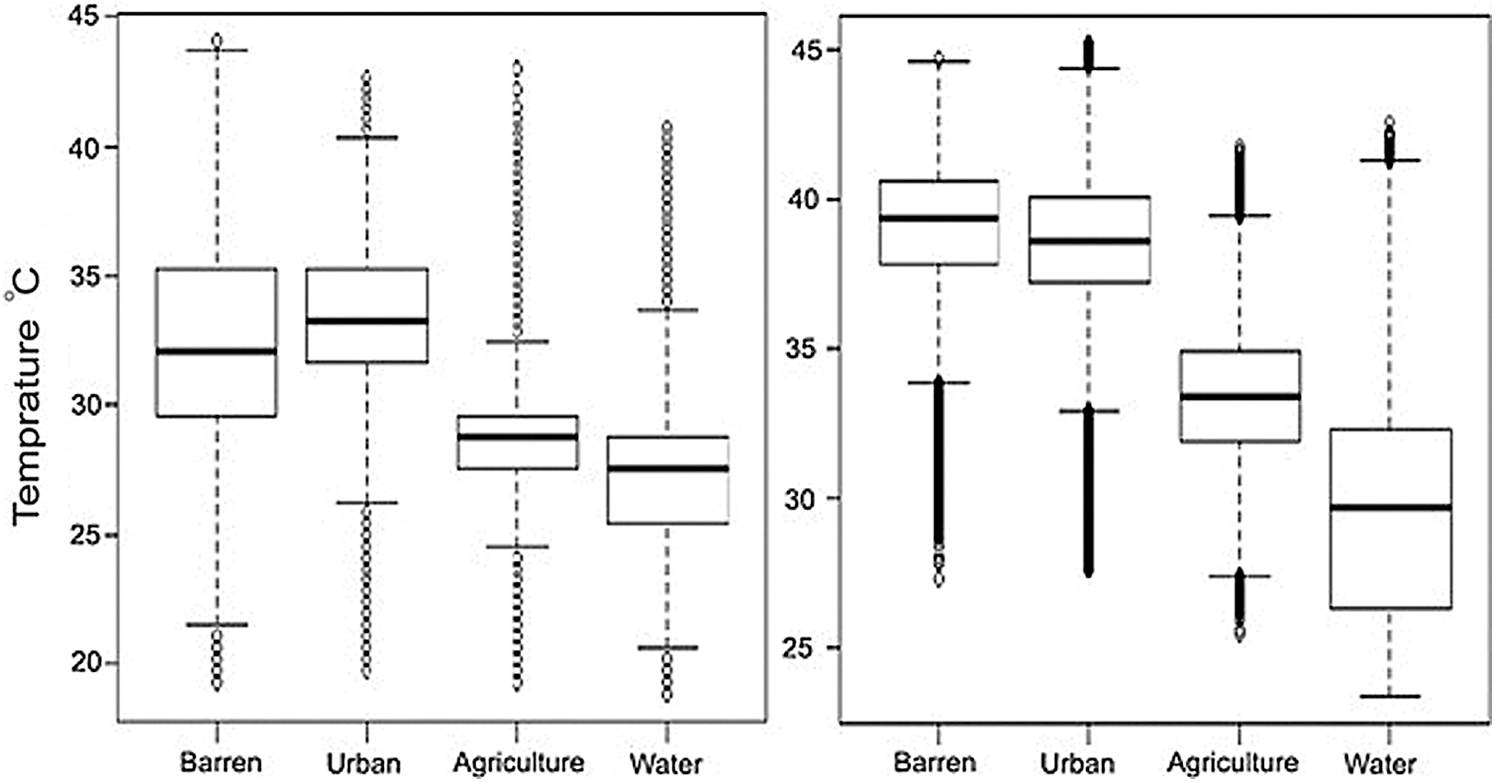
Figure 17: Land surface temperature of various land cover during 1996 and 2019

6  Comparison with Previous Works

Most of the author’s work shows a very close relationship between the change in land surface temperature and urbanization [30–32]. The current work’s main objective is the LU/LC classification using ANN and SVM and Land surface temperature extraction. Further, analyze the impact of urbanization on temperature by correlating the LU/LC classification with LST. The experiments and results of our work reveal a difference in the effects of urbanization in the LST. Specifically, the urbanization in the peripheral areas increased the LST, while in the center areas, urbanization is considered beneficial for reducing the LST with relatively high intensity. Although the authors have some work in this field, the authors carried out some valuable assessments. Imran et al. [33] showed the agricultural productivity in the Peshawar region and the influence of the land-use change valuation on surface temperature. Amin et al. [34] exposed that the LST in several high-temperature areas of the central City of Tehran declined with the development of urbanization, which is stable with the changing inclinations of districts in our study’s core region area. Jian et al. [35] evaluated the 285 Cities of china, confirming that changes in land use and spatial structures related to urban renewal significantly eradicated or weakened the intensity of UHIs. The existing research highlighted urban renewal’s effect on LST in high-building densities, high populations, and high urbanization intensity. Though, no previous work has exposed the spatial difference of urban renewal impact on LST, especially in a comparative analysis of the supervised classifiers such as ANN and SVM and the impact difference of areas with different degrees of urbanization. Therefore, the impact of urban renewal on LST in peripheral areas needs further study.

7  Conclusion

This work analyzes the impact of urbanization on land sur- face temperature in the area (Peshawar). A Negative correlation between NDVI and LST is found in the study. An increase in surface temperature is observed in fewer vegetation areas. Buildings, surface soil nature, and settlement in the central part of the site under study directly impact surface temperature. Moreover, this paper presents a comparative analysis of two states of the art algorithms, i.e., Support Vector Machine and Artificial Neural Network. Classification performed through Support Vector Machine is more accurate as compared to Artificial Neural Network. However, ANN produced good results in some more classes because of its generalization properties. Nevertheless, for land cover classification accuracy, both ANN and SVM are not much different when more training samples are provided.

Funding Statement: The authors received no specific funding for this study.

Conflicts of Interest: The authors declare that they have no conflicts of interest to report regarding the present study.

This work is licensed under a Creative Commons Attribution 4.0 International License, which permits unrestricted use, distribution, and reproduction in any medium, provided the original work is properly cited.