Computers, Materials & Continua DOI:10.32604/cmc.2022.018718
Article

Effectiveness Assessment of the Search-Based Statistical Structural Testing

Yang Shi*, Xiaoyu Song, Marek Perkowski and Fu Li

Department of Electrical and Computer Engineering, Portland State University, Portland, 97201, USA
*Corresponding Author: Yang Shi. Email: yangshi.psu@gmail.com
Received: 19 March 2021; Accepted: 26 April 2021

Abstract: Search-based statistical structural testing (SBSST) is a promising technique that uses automated search to construct input distributions for statistical structural testing. It has been proved that a simple search algorithm, for example, the hill-climber is able to optimize an input distribution. However, due to the noisy fitness estimation of the minimum triggering probability among all cover elements (Tri-Low-Bound), the existing approach does not show a satisfactory efficiency. Constructing input distributions to satisfy the Tri-Low-Bound criterion requires an extensive computation time. Tri-Low-Bound is considered a strong criterion, and it is demonstrated to sustain a high fault-detecting ability. This article tries to answer the following question: if we use a relaxed constraint that significantly reduces the time consumption on search, can the optimized input distribution still be effective in fault-detecting ability? In this article, we propose a type of criterion called fairness-enhanced-sum-of-triggering-probability (p-L1-Max). The criterion utilizes the sum of triggering probabilities as the fitness value and leverages a parameter p to adjust the uniformness of test data generation. We conducted extensive experiments to compare the computation time and the fault-detecting ability between the two criteria. The result shows that the 1.0-L1-Max criterion has the highest efficiency, and it is more practical to use than the Tri-Low-Bound criterion. To measure a criterion’s fault-detecting ability, we introduce a definition of expected faults found in the effective test set size region. To measure the effective test set size region, we present a theoretical analysis of the expected faults found with respect to various test set sizes and use the uniform distribution as a baseline to derive the effective test set size region’s definition.

Keywords: Statistical structural testing; evolutionary algorithms; optimization; coverage criteria

1  Introduction

Statistical structural testing has been studied for decades. In SST, test inputs are sampled from probability distributions (a.k.a, input distributions) over the input domain space. The distributions guarantee that a sampled test input has a probability greater than a threshold to trigger each branch cover element (BCE) under test. This criterion increases the chance of triggering BCEs associated with a small input sub-domain space, resulting in a higher fault-detecting ability than random testing [1]. Constructing such distributions is not a trivial work. A tester needs to know the input sub-domain space associated with each cover element and then assign the right probabilities to each space to create an optimal input distribution. Fortunately, this process can be automated by the search-based software testing framework.

Search-based SST(SBSST) is similar to the traditional search-based coverage-driven approaches where a test input set is refined during the system under test (SUT’s) runtime. However, SBSST optimizes an input distribution’s parameter values and uses sampled test input sets to evaluate fitness. A general evaluation criterion is the Triggering Probability Lower Bound (Tri-Low-Bound), where the minimum triggering probability among all BCEs under test is used as the fitness value. Poulding et al. [2] demonstrate the effectiveness of using the hill-climbing algorithm to search input distributions with the Tri-Low-Bound criterion. However, the time consumption on search is a significant concern. The critical issue is that the estimated triggering probabilities cause over/underestimation, which significantly misleads the search direction. Moreover, if a BCE under test is associated with a diminutive input sub-domain space, triggering the BCE is considered a rare event. The probability estimation of a rare event is usually inaccurate. We conducted a small experiment to show the problem: Our synthetic SUT has two inputs, with each consist of 30 elements. A cover element C can be triggered by 4 non-consecutive test inputs, and the sample set used to estimate fitness has 90 test inputs. We use the hill-climbing algorithm with a Tabu list to search for an input distribution that maximizes C's triggering probability. The fitness is estimated with the Wilson Score approach with continuity correction [3]. Over 5000 iterations, fitness swings around 0.01, and the confidence band ranges from near 0 to an average around 0.15, which could not provide helpful information to guide the search direction moving forward.

Tri-Low-Bound is considered a strong criterion since every BCE’s triggering probability is constrained. In this article, we answer the following question: If we use a relaxed constraint that significantly reduces the time consumption on search, can the optimized input distribution still be effective in fault-detecting ability? We propose a new criterion called fairness-enhanced-sum-of-triggering-probability (p-L1-Max). Instead of Tri-Low-Bound, the sum of triggering probabilities could reduce the noisy fitness influence by estimating the group of events. However, it causes the search direction biasing to one input sub-domain space, whereas the rests take zero chances to be sampled. Hence, we also take fairness a parameter p into consideration, which tunes the distribution to be uniform.

A question raised is how to compare two criteria. In SST, test inputs are sampled from distributions, and the test set size is proportional to fault-detecting ability. This article provides a theoretical analysis of the fault-detecting ability in terms of various test set sizes. We use the uniform distribution as a baseline to derive the effective test set size region R where SST outperforms random testing and determine the expected faults found in R as the effectiveness measure of criteria. To compare two criteria, we use the effectiveness-to-cost ratio, where cost is the wall-time on search.

The main contributions are concluded as the followings. First, we present a method called effectiveness-to-cost ratio to evaluate the fault-detecting ability of criteria for SST problems. Second, we proposed a new criterion(p-L1-Max) and conducted a series of experiments to compare the proposed and traditional criteria. Our results show that the proposed criterion has a better effectiveness-to-cost ratio, and it is more realistic in practical uses.

This paper is organized as follows. Section 2 provides the related work. Section 3 provides the formal definition of input distribution’s effectiveness. Section 4 provides the formal representation of SBSST. Section 5 describes the Criteria under evaluation. Section 6 provides the experimental study. Section 7 gives the conclusion.

2  Related Work

The traditional coverage-oriented test data generation has been widely studied for decades. In those studies, people believe that a test set that achieves a higher coverage provides a more thorough test indicating a stronger fault-detecting ability [4]. However, Tasiran pointed out that the through tests may not provide a high fault-detecting ability [5]. Also, even a coverage criterion subsumes another, the test data set that satisfies the first criterion does not necessarily prove the stronger fault-detecting ability. The lack of randomness using the traditional method is one of the reasons causing low fault-detecting rate. Since the coverage criteria require a fixed number of tests for each cover element, there is no chance that a particular cover element can be triggered multiple times than another. However, the chances are beneficial for detecting faults. In the early work, Duran et al. [6] performed the cost-effective analysis for random testing. They showed that the random testing demonstrates a higher fault detecting ability over branch testing for some fault programs that have critical errors that can be discovered with a low failure rate. To combine the randomness and the traditional coverage adequacy into test data generation, Thevenod-Fosse created a new method, called Statistical Structural Testing (SST). In SST, test inputs are sampled from a probability distribution over the input domain space. The distribution guarantees that the sampled test inputs have probabilities at least greater than a pre-defined value to trigger each cover element (a.k.a, the triggering probability lower bound). They compared the fault-detecting power from the three approaches: deterministic, random, and SST by using mutation testing technique [7]. The experiment results demonstrate that the test set generated by SST is superior efficacy in detecting software fault. Constructing an optimal input distribution that satisfies the probabilistic coverage is not a trivial work. A tester needs to know the knowledge of the sub-input domain space associated with each cover element. Then he needs to assign proper probabilities to each sub-input domain space to create an optimal input distribution. However, as the computing power increases dramatically in recent years, the Search-Based Software Testing (SBST) framework has gained much attention. SBST refers to a software testing methodology that automates the test data generation process using intelligent search algorithms. It is often a dynamic testing process, meaning that the test set is refined during the SUT’s run-time. A typical contribution made by Tracey et al. [8] used G.A to build the test set against the branch coverage criteria. Up to now, there are plenty of Meta-heuristic algorithms dedicated to generating test input set [9–13]. The SBST framework for SST problems is firstly studied by Poulding and Clark. They modeled the input distribution as a Bayesian Network, with nodes represented as inputs, the values in each node defined as a collection of sub-input domain spaces. Their objective is to optimize the Bayesian network’s parameters such that the sampled inputs achieve a probability lower-bound of triggering each branch. They used the hill-climbing as the search algorithm. Their experiment results demonstrated the practicality of applying the SBST framework for producing an optimal input distribution. However, their experiment results also show that efficiency is still a crucial issue. Based on their research, we analyze the problem that causes the low-efficiency issue and proposed the new criterion p-L1-Max.

3  Effectiveness Estimation of Input Distributions

An optimized input distribution is a biased uniform distribution. The point of biasing the uniform distribution is to detect faults more effectively than random testing. Given a test set size, if the number of faults found by the uniform distribution outperforms or equal to the biased input distribution, the biased input distribution should have no effectiveness, since random testing does not require the input distribution construction process. Hence, to investigate an input distribution's effectiveness, we should determine the effective test set sizes.

3.1 Effective Test Set Size

To find effective test set size theoretically, we adopt Duran’s fault revealing ability model. Suppose that an input domain space is re-organized into many consecutive, non-overlapped subsets. In each subset, the test inputs are uniformly selected. Let θi be the failure rate of the i-th partition, which refers to the probability that a randomly selected input triggers the system failure. Let pi be the probability of selecting the i-th partition, k be the total number of partitions and n be the test set size. The expected number of errors found under the assumption that each partition contains one error is formulated as follows:

For a uniform input distribution, pi=1k,∀i∈{1,…,k}. Then, the effectiveness of a biased input distribution is the following:

E=Eb−Er=∑i=1k(1−1kθi)n−∑j=1k(1−pjθj)n (1)

We are interested in the maximum and minimum of E with respect to various n. This function is a summation over exponential functions. An intuitive re-formation can be done as follows: Suppose that a set U={(1−1kθ1),…,(1−1kθk)}, a set B={(1--p1θ1),…,(1−pkθk)} and C(x) is an indication function that C(x)=1 if x∈U; C(x) = −1 if x∈B. Then, Eq. (1) can be written as follows:

E=∑α∈U∪BC(α)αnα∈[0,1] (2)

Shestopaloff [14] proves the following corollary of the above function: “if there exists a sequence of α such that 0<αN,…,α0<1,C0>0. This series can change its algebraic sign a maximum of two times. It can have a maximum of two extrema. It monotonically converges to zero after the second extremum, which is always a maximum.” α0 refers to the maximum fault-detecting rate of a partition, it can be either from U or B. We analyze them separately. Let Ti denote index sets that stores indexes for U and B. Specifically,

Suppose that α0 is an element in {Ui∣i∈T1}. Forming an order over U∪B with one algebraic sign change is impossible. With two algebraic sign changes, the sequence should be the following:

where “>\prime\prime indicates that any element in the left set is greater than any element in the right set. This ordering relation reflects a type of input distributions. The top graph in Fig. 1 shows an example of effectiveness function which satisfies the above sequence. The difference curve drawn from Eq. (1) shows its maximum at the test set size marked by the dashed line. It monotonically converges to 0 after the maximum.

Figure 1: Three typical effectiveness functions from theoretical perspective

Suppose that the maximum value α0 is an element in {Bi∣i∈T2}. Then, the sequence with two algebraic sign changes is

It is noted that C0 is a negative number. To applying the shestopaloff’s corollary, the indication function outputs the opposite number, and the output E should multiply −1 to coincide with the original output. The Fig. 1’s leftmost graph shows an example of an effectiveness function that satisfies the above sequence. The zero-effectiveness test set size is marked by the blue dashed line. After this point, the uniform distribution outperforms the biased input distribution. The maximum effectiveness test set size is marked by the red dashed line. If a sequence contains more than two algebraic sign changes, a possible outcome can be depicted by the rightmost figure of Fig. 1. For this case, there is only one extreme, and it is a maximum.

Hence, for three situations in above, each effectiveness function shows a maximum effectiveness test set size. Further, we can conclude that there is a range of test set sizes that the effectiveness of biased input distribution outperforms the uniform distribution, and we call it the effective region. Formally, Let nm denotes the test set size at the maximum effectiveness an ns,ns>nm denotes the test set size at the zero or minimum effectiveness. The effective region, denoted by R, ranges within [nm,ns]. Then the effectiveness for a coverage criterion, which measures the average number of faults found per test for each test set in the effective region is defined as follows:

η=1ns−nm+1∑k=nmns1k∗Eb (3)

In the later assessments of criteria, for each system under test (SUT), we estimate ns,nm and Eb, and calculate the effectiveness based on Eq. (3).

3.2 Estimation of Expected Errors Found Eb

To estimate the expected errors found, we use 32 test sets sampled with replacement from the input distribution. Each test set runs against the mutation testing tool, named Milu [15], to retrieve mutation scores. The averaged 32 sets of mutation scores are calculated to estimate the expected errors found by an input distribution at each test set size.

Mutation testing is a software testing method dedicated to evaluating the effectiveness of a test set. In mutation testing, a SUT is mutated into a set of mutants. Each mutant is a copy of the SUT injected with an artificial fault. A test input is said to kill a mutant if one of the mutant's execution results is different from the original SUT. A mutant that produces the same result as the original SUT is called an equivalent mutant. Mutation score, defined as the percentage of the killed but excepting the equivalent mutants, is an estimation of the expected errors found (i.e., fault-detecting ability) by a test set.

3.3 Estimation of the effective region R

With the given sets of mutation scores at each test set size, we perform the least-square regression on the data set to create estimation functions of fault detecting ability with the test set size n for both biased input distributions and the uniform distributions. To find the effective test set region with strong confidence, we perform hypothesis testing on the data set. It is difficult to fit the data into Eq. (1) which is a sum of exponential functions. Instead, we created an exponential function model presented in the following to best fit the averaged mutation scores at each test size:

where {a1,…,a4} are the learning parameters, pl,n are the training variables where pl denote the percentage of living mutants left, which is equal to 1−ms and n denotes the test set size. The reason not to directly applying mutation score is that the exponential functions are convex with ms≥0, whereas the Eq. (1) is concave. The function model is a gamma distribution without the normalization constant.

{a2,a3,a4} are the parameters used to shift or scale the input and output. Hypothesis testing makes statistical inference on mutation score sets when comparing the effectiveness of the uniform and biased input distributions at each test set size. If there is no significant evidence showing either one performs better, even with the difference shown by the estimated curves, their effectiveness is treated as equal. We perform a one-tailed hypothesis testing with the Wilcoxon rank-sum test [16] on the two mutation score sets at each test set size. The confidence level is 0.05. Specifically, the hypotheses are:

•   H0: there is no significant difference between mutation scores that produced by random testing and input distributions constructed from an evaluation metric.

•   H1: The mutation scores produced by random testing is significantly different from mutation scores produced by input distributions constructed from an evaluation metric.

To determine the effective set size region, we present Algorithm 1. If there is no test set size such that the corresponding p-value is less than 0.05, the biased input distribution is indifferent from the uniform distribution on the fault detecting ability at any test set size that below the maximum set size. Otherwise, the learned functions fb,fu are used to mathematically derive the test set size at the maximum effectiveness tsmax and the zero-effectiveness set of test set sizes tsmin. If the p-value at tsmax is less than 0.05, nm is determined to be tsmax. If there exists a test set size t in tsmax such that t is greater than nm, then ns is determined to be t.

4  Search-Based Statistical Structural Testing

In this section, we provide a formal representation of SBSST. In SST, a SUT is essentially treated as a control flow graph where each node represents a linear sequence of basic blocks, and each edge represents the flow of the basic blocks [17]. In the context of structural testing, an edge is also known as a branch cover element (BCE). A BCE is said to be triggered by an input x if the path in CFG executed by x contains the corresponding edge. Hence, for the entire input domain space D, there exists a subset of the input domain space that triggers each BCE. Suppose the BCE ci is under test. P(x) denotes a discrete probability distribution over the input domain space. The probability of triggering the BCE ci is the sum of the probabilities of each input in Dci. However, it is not possible to enumerate all inputs to derive the triggering probability. Therefore, we estimate the triggering probabilities derived from the sampled input set. Suppose the sampled set size is n, and the test size triggers ci is nci. The estimated triggering probability of ci is ncin.

4.1 Input Distribution Model

We choose the sum of the weighted uniform distributions as the input distribution model, which is formally defined as follows:

where the weight vector w satisfies:

U(x) is a multi-dimensional uniform distribution whose dimension equals the input domain space’s dimension. The uniform distributions are applied on the consecutive, none-overlapped sub-input domain spaces, denoted as S1,…,Sku.

4.2 Input Distribution Construction

We view the input distribution construction shown in Fig. 2 as a two-step process: First, we arrange sub-input domains to each uniform distribution’s boundary. Second, we assign weights to the uniform distributions. In each iteration, the genetic operators produce an arrangement to form a new set of uniform distributions. Each uniform distribution generates a sampled input set to run with SUT to estimate triggering probabilities. Then, we apply numerical optimization methods to derive the best weights from the estimated triggering probabilities to maximize the overall triggering probabilities. The purpose of adopting the Genetic Algorithm (G.A) is to search for the best arrangement. The detail of G.A is described as follows.

•   Encoding: The chromosome is encoded as an array of integers. Each integer δi represents the size of an input-subdomain space. The lower boundary li of the i-th uniform distribution equals ∑k=0i−1δk. The upper boundary ui of the i-th uniform distribution equals li+δi.

•   Recombination: We adopt the two-point crossover strategy. The two-point crossover randomly selects two positions from two individuals and swaps the contents between them. The crossover rate setups to 0.9.

•   Mutation: We adopt the uniform mutation strategy. The uniform mutation operator mutates a gene by randomly picking up an input set and assigning the index of the input set into the gene. Each gene has a probability of 0.8 to be mutated.

•   Selection: We adopt the roulette-wheel selection strategy with elitism for reproduction. Elitism is applied to ensure the best solution in the current iteration is still available for reproduction in the next generations.

•   Fitness Evaluation: The fitness function depends on the criterion, which is described in later section.

•   Stop criteria: The main loop continues until one of the two stop conditions is satisfied. First, the fitness does not improve over the last 100 iterations. Second, the number of iterations reaches a pre-set maximum value.

Figure 2: The overall workflow

5  Fitness Criteria

This section provides formal definitions of Tri-Low-Bound and p-L1-Max criteria and shows how to use numerical optimization methods to derive the weight vectors. Before start, we reformulate the triggering probabilities to matrix form. The triggering probabilities in all subdomains can be written in a matrix form, denoted by A, where each column represents a subdomain in the set S, and each row represents a BCE. The value aij of the i-th row and the j-th column is the triggering probability of the BCE cI in Sj.

Given a matrix A, the triggering probability vector Pc→ is the linear combination of the column vectors with scalar vector w:

Pc→=[a11⋮am1]ω1+[a12⋮am2]ω2+⋯+[a1ku⋮amku]ωku (4)

where ku denotes the number of components in the input distribution model. Ku is set to m, which refers to the number of BCEs (i.e., the row counts of matrix A).

5.1 Tri-Low-Bound

The Tri-Low-Bound criterion for statistical structural testing originates from the definition of the statistical test set quality, which is defined as the minimum probability of triggering a cover element by a test set. Formally,

Tri-Low-Bound = min{Pc1,…,Pcm}

5.2 p-L1-Max

The proposed p-L1-Max criterion evaluates an input distribution based on the estimated sum of triggering probabilities, and the input distribution must satisfy the fairness property. According to Eq. (4), the sum of triggering probabilities, denoted by fA(w) can be derived by adding up the dot product of each row vector of matrix A and the weight vector:

Since the weight vector is constrained, we can view the above equation as a m-Simplex. The maximum value L1-Max is equal to the maximum sum of column vectors of matrix A:

Hence, the weight associated with the maximum sum of column vectors equals 1.0. The weights associated with the rest columns are 0.0. This situation brings up the fairness issue, where only the subdomain associated with the maximum weight can be sampled. The rest have no chance to be sampled.

It is the fact that the uniform distribution is the fairest distribution since each input has equal probability to be sampled. Hence, we define the fairness property as the L2-distance from the input distribution to the uniform distribution. We use a parameter p to manually adjust the importance of the two objectives. In this way, the input distribution generation process can be tuned to bias on L1-Max or the fairness. The formal definition of criterion p-L1-Max is defined as follows:

In this study, we use the following values for the tuning parameter p: p∈{0.2,0.4,0.6,0.8,1.0}. The optimization objective becomes to minimize the L2-distance of the input distribution and the uniform distribution, with constraints that the estimated sum of triggering probabilities should be at least greater than the proportion of the maximum sum of triggering probabilities.

5.3 Weights Calculation for Tri-Low-Bound

The fitness measure for Tri-Low-Bound is the minimum value in the triggering probability vector Pc→.

Our objective is to optimize the weight vector such that the minimum value in the triggering probability vector is maximized. The problem of Maximizing the inner minimum is equivalent to the following linear programming problem where the objective is to maximize the variable v with respect to weight vector w. Specifically, the optimization problem is defined as follows:

This is a standard linear programming problem. We selected to use the active set method provided in ALGLIB [18] to solve the problem.

5.4 Weights Calculation for p-L1-Max

The fitness for criterion p-L1-Max is measured by the sum of estimated triggering probabilities with p∗L2-distance constraint. The tuning parameter p whose value can be categorized into three types:

•   p=0: Any feasible weight vector satisfies the constraint ∑iPci≥0. The L2-distance is 0. The derived input distribution is a uniform distribution.

•   p=1: The constraint ∑iPcIequalsL1−Max. Then, it is not necessary to minimize the L2-distance. The fitness equals L1-Max.

•   p>0 & p<1: see below.

We treat the optimization problem as a Constrained Quadratic Programming (CQP) problem which can be solved by the active set method. To form the problem as a CQP problem, we construct the quadratic matrix Q and the linear vector H. After expanding the L2-distance equation, matrix Q becomes a diagonal matrix with elements qI,i=2∗|Si|−2,∀i∈{1,…,m}. The vector H has elements hi=−2∗|Si|−1∗|S|−1,∀i∈{1,…,m}.

The whole process to optimize the weight vector starts from checking the value of p. If p equals 0, the process finishes and outputs the uniform distribution. If p equals 1, the process ignores the fairness property and uses L1-Max as the fitness. If p is between 0 and 1, the process first forms matrix Q and vector H and then it applies the active set method to derive the optimal weight vector w→∗.

6  Experiments

Our experiment’s objective is to compare the effectiveness-to-cost ratios of SSBST by adopting different criteria. Hence, we naturally divided the experiments into three sections: the effectiveness, the search run-time, and the effectiveness-to-cost ratio sections. For criterion p-L1-Max, we select p={0.2,0.4,0.6,0.8,1.0} for study. We implemented the G.A by C++ and C# under the Windows 10 environment. We use the mutation testing tool under Ubuntu 12. The hardware configuration is IntelCore i7-4770K 3.50 GHz with 16 GB DDR3 memory. We continue to use the benchmark programs provided by Poulding that are sufficient for our research purpose. The characteristics are shown in Tab. 1. NLOC denotes the number of lines of code. CCN denotes the Cyclomatic complexity of a SUT. NBC denotes the number of branches of a SUT. Param denotes the number of input variables. Triangle and Nichneu can be found in [19,20].

6.1 Effectiveness

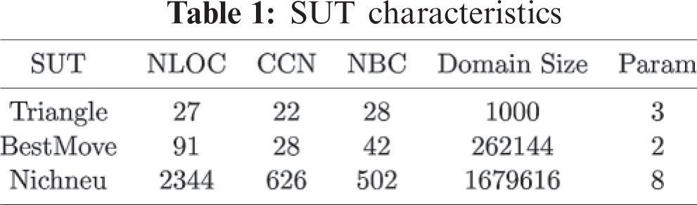
6.1.1 Regression Goodness of Fit

The effectiveness measure requires the estimation of nm and ns. We performed regression analysis on the proposed exponential model for uniform and biased distribution’s test data sets to find the values. The goodness of fit of the regression model is represented by the Root Mean Square Error shown in Tab. 2.

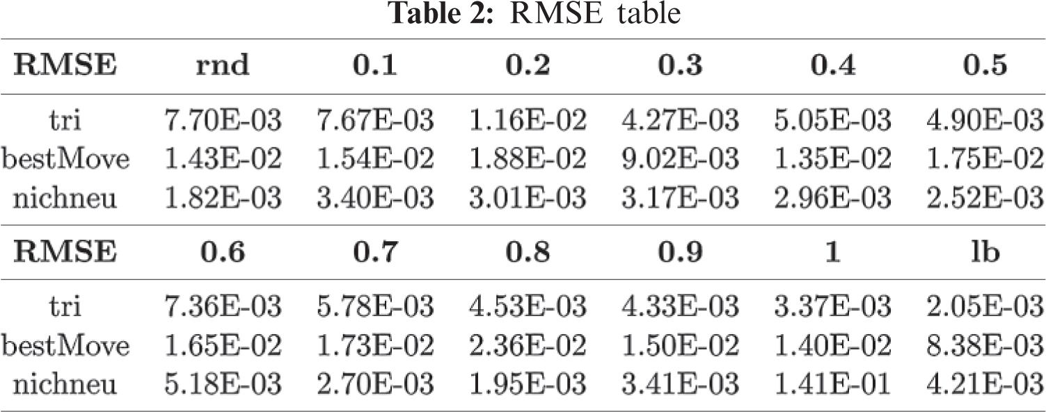
In general, the smaller RMSE, the fitter the estimated model. If the RMSE value is smaller or equal to 0.3, the estimated model is acceptable [21]. In Tab. 2, the maximum value is 0.141, and the averaged value is 0.0117, which is far less than 0.3. Hence, our model can accurately predict the expected number of errors found with different test set sizes.

6.1.2 Estimating nm and ns

We use Algorithm 1 to determine nm and ns. Speaking in detail, Fig. 3 shows the function curves and the p-values at each test set size for the three coverage criteria on the three SUTs. The dashed blue line represents the calculated test set size at nm, and the dashed yellow line represents the calculated test set size at ns. For Triangle SUT, p-values on all coverage criteria have a pyramidal peak shape, which indicates that the mutation scores of biased and uniform distributions are significantly different on the left side and right side of the peak. The inflection points of the peaks, which p-values are at least greater than 0.9 are the test set sizes that ns is mostly located. By solving the two learned functions mathematically, it can be seen that ns is very close to the inflection point. p-value at nm is less than 0.05. For BestMove, the p-values for all coverage criteria are decreasing as the test set size increases. The Tri-Low-Bound criterion shows the highest decreasing speed. It is observed that the difference between the two functions is gradually diminishing after the test set size passes nm. Hence, it can be inferred that after the maximum test set size, which is set to 100, there exists a pyramidal peak on the p-value. For Nichneu, the p-values behave differently for each coverage criteria. The p-values in 0.2-L1-Max are all above 0.05 which indicates that the biased input distribution is indifferent from the uniform distribution in detecting faults. The p-values in 1.0-L1-Max have a pyramidal peak shape, and ns is located near the inflection point. The p-values for Tri-Low-Bound have multiple local optima, which indicates that ns is in a relatively large test set size interval than the unique global optima. Above all, the estimated nm and ns matches the observations from the figures. The detailed assessment data for all the coverage criteria are shown in Tabs. 3–5 respectively.

Figure 3: Estimated effectiveness graphs for Tri (first row), BestMove (2nd row) and Nichneu (3rd row)

The column p-value<0.05 is true if there is a significant difference between biased and uniform distribution. It is observed that 0.2, 0.4, 0.6 and 0.8-L1-Max criteria does not show any difference for Nichneu. After analyzing the SUT, we noticed that the artificial faults can be triggered only by a few partitions of input-domain space, and this is the limitation of using mutation testing to estimate the triggering probabilities. However, for Tri and BestMove, such difference is obvious. The column Improvement% shows the percentage improvement on mutation scores from the uniform distribution at the test set size nm. We observe that the Tri-Low-Bound is significantly superior to any p-L1-Max coverage criteria except for the Triangle. We suspect the estimation error on nm which rounds up to integer, causes 1.0-L1-Max outperforms Tri-Low-Bound with 15% lead. Besides this, we recognize the following criteria order on maximum effectiveness:

Tri-Low-Bound ≥ 1.0-L1-Max ≥,… , 0.2-L1-Max

6.1.3 Effectiveness

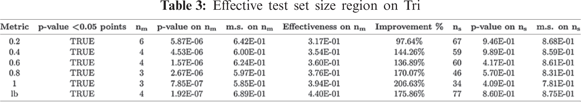
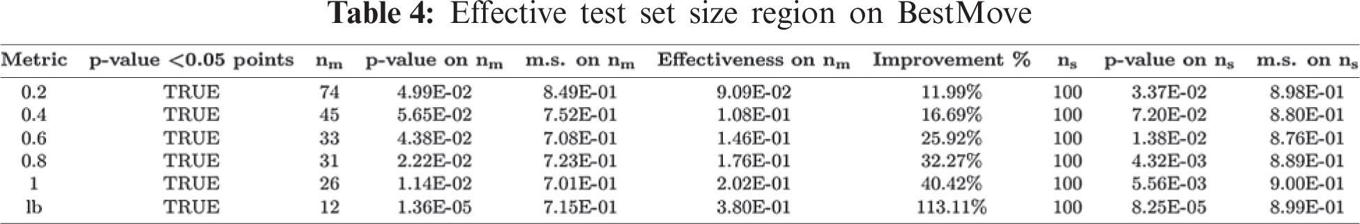
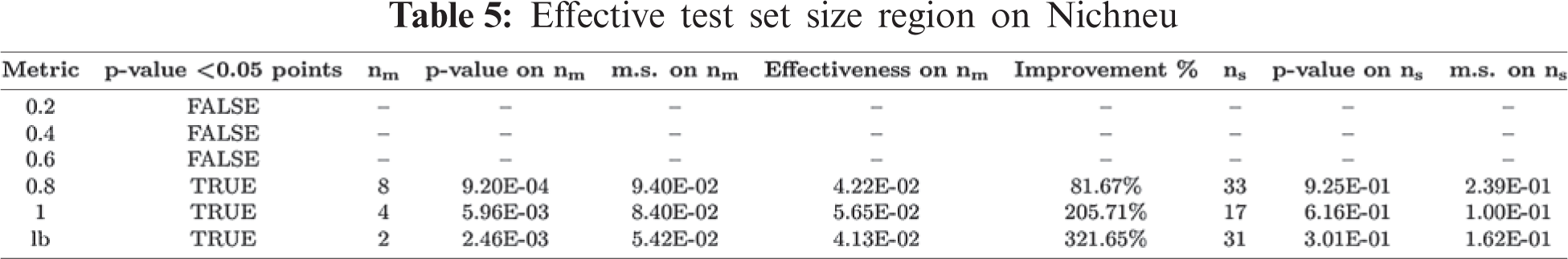
The effectiveness measure η, defined in Eq. (3), represents the average number of errors found per test in the effective test set size region. The effectiveness data is shown in Tab. 6. For Triangle and Nichneu, the 1.0-L1-Max coverage criterion outperforms the Tri-Low-Bound criteria by 68.22 and 10.33 respectively. For BestMove, Tri-Low-Bound outperforms 1.0-L1-Max, since the actual ns beyond 100. Above all, we conclude that 1.0-L1-Max outperforms Tri-Low-Bound. We noted that as the cyclomatic complexity increases, the superiority of Tri-Low-Bound is decreasing. Also, adding more fairness into the input distribution construction process does not benefit the fault-detecting ability. We believe this is due to the weakness of using mutation testing to evaluate the fault-detecting ability. A real software bug is sometimes much more difficult to discover than a bug automatically generated from a template. Hence, increasing test diversity is important in real-world usages.

6.2 Search Results

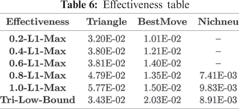
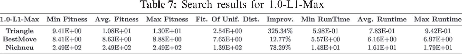
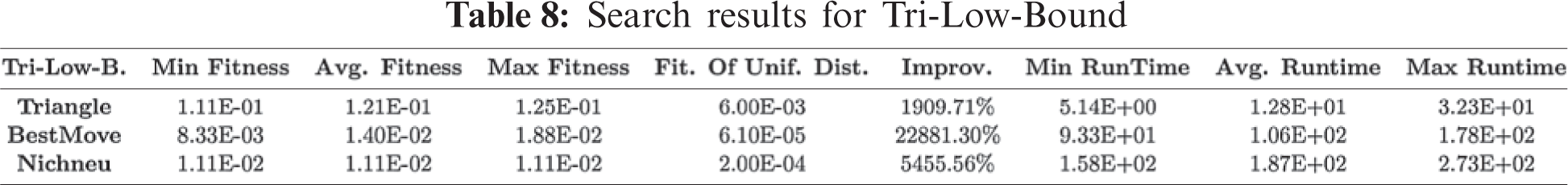
We solely present the 1.0-L1-Max criterion’s search result, since 1.0-L1-Max requires the least computation time in the family of p-L1-Max criteria. The results are shown in Tabs. 7 and 8. The first five columns show the fitness statistics. The column Fit. Of Unif. Dist shows the fitness values for the uniform distribution. The column Improv. shows the increment in the percentage of the average fitness of an optimized input distribution over the uniform distribution. We observed that the fitness improvement is much more significant by using the Tri-Low-Bound criterion. The last four columns present the computation time statistics. For each SUT, the average computation time for the Tri-Low-Bound criterion is greater than the 1.0-L1-Max criterion.

6.3 Effectiveness-to-Cost Ratio

The effectiveness-to-cost ratio measures the criterion’s efficiency on fault-detecting ability, it is expressed as a fraction of the effectiveness over the search time. In Fig. 4, for all SUTs, the efficiency for 1.0-L1-Max is significantly greater than the Tri-Low-Bound. For p-L1-Max coverage criteria, the efficiency decreases as p decreases. Except for Nichneu, where 0.2, 0.4, 0.6-L1-Max exposes no efficiency (uniform outperforms biased distributions), p-L1-Max shows a higher efficiency value than Tri-Low-Bound. Hence, we conclude that the search algorithm by using the 1.0-L1-Max coverage criterion has the most excellent efficiency in detecting software faults than any other criterion. The Tri-Low-Bound has the least efficiency due to the significant computation time required to search for the optimal input distribution.

Figure 4: Effectiveness-to-cost ratio for investigated coverage criteria

7  Conclusion

The current search-based statistical structural testing has its limitations on efficiency. The primary reason is the noisy fitness estimation of triggering probabilities. This paper aims to improve efficiency by investigating criteria. We proposed a new criterion, called p-L1-Max, and conducted experiments to compare the efficiency of input distributions produced against the p-L1-Max and the traditional Tri-Low-Bound criterion. The experiments show that 1.0-L1-Max provides the highest effectiveness and efficiency. However, the fault-detecting abilities to find real bugs is different from the template bugs. Hence, the tuning parameter p to adjust the test diversity is equally essential.

Funding Statement: Publication of this article in an open access journal was funded by the Portland State University Library’s Open Access Fund.

Conflicts of Interest: The authors declare that they have no conflicts of interest to report regarding the present study.

This work is licensed under a Creative Commons Attribution 4.0 International License, which permits unrestricted use, distribution, and reproduction in any medium, provided the original work is properly cited.