Computers, Materials & Continua DOI:10.32604/cmc.2022.018270
Article

Human Gait Recognition Using Deep Learning and Improved Ant Colony Optimization

Awais Khan1, Muhammad Attique Khan1, Muhammad Younus Javed1, Majed Alhaisoni2, Usman Tariq3, Seifedine Kadry4, Jung-In Choi5 and Yunyoung Nam6,*

1Department of Computer Science, HITEC University Taxila, Taxila, 47080, Pakistan
2College of Computer Science and Engineering, University of Ha'il, Ha'il, Saudi Arabia
3College of Computer Engineering and Sciences, Prince Sattam Bin Abdulaziz University, Al-Khraj, Saudi Arabia
4Faculty of Applied Computing and Technology, Noroff University College, Kristiansand, Norway
5Department of Applied Artificial Intelligence, Ajou University, Suwon, Korea
6Department of Computer Science and Engineering, Soonchunhyang University, Asan, Korea
*Corresponding Author: Yunyoung Nam. Email: ynam@sch.ac.kr
Received: 03 March 2021; Accepted: 07 May 2021

Abstract: Human gait recognition (HGR) has received a lot of attention in the last decade as an alternative biometric technique. The main challenges in gait recognition are the change in in-person view angle and covariant factors. The major covariant factors are walking while carrying a bag and walking while wearing a coat. Deep learning is a new machine learning technique that is gaining popularity. Many techniques for HGR based on deep learning are presented in the literature. The requirement of an efficient framework is always required for correct and quick gait recognition. We proposed a fully automated deep learning and improved ant colony optimization (IACO) framework for HGR using video sequences in this work. The proposed framework consists of four primary steps. In the first step, the database is normalized in a video frame. In the second step, two pre-trained models named ResNet101 and InceptionV3 are selected and modified according to the dataset's nature. After that, we trained both modified models using transfer learning and extracted the features. The IACO algorithm is used to improve the extracted features. IACO is used to select the best features, which are then passed to the Cubic SVM for final classification. The cubic SVM employs a multiclass method. The experiment was carried out on three angles (0, 18, and 180) of the CASIA B dataset, and the accuracy was 95.2, 93.9, and 98.2 percent, respectively. A comparison with existing techniques is also performed, and the proposed method outperforms in terms of accuracy and computational time.

Keywords: Gait recognition; deep learning; transfer learning; features optimization; classification

1  Introduction

Human identification using biometric techniques has become the most important issue in recent years [1]. Human identification techniques based on fingerprint and face detection are available. These techniques are used to identify humans based on their distinguishing characteristics. Every person has unique fingerprints and iris patterns that are used for identification [2]. Scientists are increasingly interested in human gait as a biometric approach [3,4]. In comparison to fingerprint and face recognition technologies, gait recognition has a more beneficial system. Automatic human verification and video surveillance are two important applications of gait recognition [5,6]. The HGR has recently developed a dynamic study zone in biometric applications and has received significant attention in Computer Vision (CV) research [7]. Gait is a common and ordinary behavior of all humans, but it is a very complex process because it works with the association from an examination standpoint. The human gait recognition process is divided into two approaches: model-based and model-free [8].

The model-based approach directs human movement based on prior knowledge [9], whereas the model-free approach generates sketches of the human body known as posture generation or skeletons [10]. The model-based approach analyses human behaviors based on joint movement and upper/lower body parts. The model-free approach, on the other hand, is simpler to implement and requires less computational time. Many computerized techniques are used in the literature to automate this application [11]. Computer vision researchers used methods based on both classical and deep learning techniques. In traditional techniques, recognition is accomplished through a series of steps such as data preprocessing, segmenting the region of interest (ROI), feature extraction, and classification. The authors used contrast enhancement techniques during the preprocessing step [12]. In the following step, several segmentation techniques are used to extract the ROI. This is followed by the features extraction step, which extracts texture, shape, and point features. These features are enhanced further by feature reduction techniques such as PCA, Entropy, and a few others [13]. In recent years, the introduction of deep learning into machine learning has demonstrated great success in a variety of applications, including biometrics [14], surveillance [15,16], and medicine [17,18]. A simple deep learning model did not necessitate preprocessing or the use of raw data. Several hidden layers are used to extract the features. Convolutional layers, ReLU layers, max-pooling, and batch normalization are examples of hidden layers. The features are combined in one dimension at fully connected layers classified as Softmax layers [19].

Mehmood et al. [20] presented a novel deep learning-based HGR framework. The presented method consisted of four significant steps: preprocessing of video frames, modification of pre-trained deep learning models, exploiting only the best features with a firefly algorithm, and finally, classification. In this work, the fusion is also used to improve the representation of extracted features. The experiment was carried out on three CASIA B dataset angles: 18, 36, and 54. The calculated accuracy for each angle was 94.3 percent, 93.8 percent, and 94.7 percent, respectively. Anusha et al. [21] used optimal binary patterns to implement the HGR. They considered the problem of view-invariant clothing and conditions. MLOOP is the name given to the extracted binary patterns. They used MLOOP to extract histogram and horizontal width features and then reduced the irrelevant ones using a reduction technique. Two datasets were used in the experimental process, and they performed admirably. Arshad et al. [22] presented a deep learning and best features selection approach for HGR with various view invariants and cofactors. Two pre-trained models were used in this method, which was modified for feature extraction. In the following step, parallel approach-based features are fused and improved further using fuzzy entropy and skewness-based formulation. The experiment was carried out on four available datasets and yielded accuracy rates of 99.8, 99.7, 93.3, and 92.2 percent, respectively. Sugandhi et al. [23] proposed a novel HGR method based on frame aggregation. This work presents two features: the first is designed using dynamic variations of human body parts, and the second is based on first-order statistics. The frames in the first feature are divided into block cycles. The features level fusion is used in the final and executed classification. The experimental process was carried out on the CASIA B dataset and resulted in improved accuracy.

Based on these studies, we consider the following challenges of this work: I change in human view angle; ii) change in a human wearing condition such as clothes, etc.; iii) change of human characteristics during walking styles such as slow walk, fast walk, etc.; iv) deep learning model requires a large amount of data to train a good model, but it is not always possible to obtain data due to various factors. We proposed a new deep learning and Improved Ant Colony Optimization framework for accurate HGR to address these issues.

•   In terms of fully connected layers, modified two pre-trained models, VGG16 and ResNet101, and added a new layer with the connection of the preceding layers.

•   A features selection technique is proposed name improved ant colony optimization (IACO). In this approach, features are initially selected using ACO and then refined using an activation function based on the mean, standard deviation, and variance.

•   Used the IACO on both modified deep learning models to compare accuracy. The best one is considered for the final classification based on accuracy.

2  Proposed Methodology

This section describes the proposed human gait recognition method. Fig. 1 depicts the main flow diagram of the proposed approach. Preprocessing datasets, feature extraction using pre-trained models, feature optimization, and classification are the main steps in this method. Deep transfer learning is used to modify two pre-trained models, Resnet 101 and Inception V3. The features are then extracted from both modified models. We get two resultant vectors as a result, which are then optimized using improved ant colony optimization (IACO). Finally, the final features are classified using multiclass classification methods.

Figure 1: Proposed architecture diagram for HGR using deep learning and IACO algorithm

2.1 Dataset Collection and Normalization Details

CASIA B [24] is a large multiview gait dataset that was created in January of 2005. 124 subjects are involved in the collection of this dataset. The dataset was captured by all subjects using the 11 different view angles. This dataset includes three deviations: changes in view angle, changes in clothing, and changes in carrying objects. This dataset contains three classes: walk with a bag, normal walk, and walk with a coat. We consider three angles in this work: 0, 18, and 180. Three conditions are included for each angle: bag carrying, normal walking, and wearing a coat. Fig. 2 shows a few examples of images from this dataset.

Figure 2: Sample frames of CASIA B dataset [24]

2.2 Convolutional Neural Network (CNN)

Deep learning demonstrated massive success in the classification phase of machine learning [25,26]. The convolutional neural network (CNN) is a deep learning technique. Using a convolutional operator, image pixels are convolved into features in this network. It aids us in image recognition, classification, and object detection. When compared to other classification algorithms, it requires very little preprocessing. CNN uses an image as input and then processes it through the hidden layers to classify it. The training and testing process will go through several layers, including a convolutional layer, a pooling layer, an activation layer, and a fully connected layer.

2.2.1 Convolutional Layer

Suppose we have some P×P fair neuron in the layers. Consider, we have n×n filter ω; then the convolutional layer has an output of (P−n+1)×(P−n+1). To calculate the pre-nonlinearity input to some unit xijl in the layer, it is defined as follows:

xijl=∑a=0n−1∑b=0n−1ωaby(i+a)(j+b)l−1(1)

2.2.2 ReLU Layer

ReLU layer is an activation layer used for the problem of non-linearity among layers. Through this layer, the negative features are converted into zero values. Mathematically, it is defined as follows:

f(x)=max(0,x)(2)

f(x)={0,if x<0x,if x≥0}(3)

2.2.3 Batch Normalization

The batch normalization is achieved through the normalization step that fixes each of the inputs layer's means and variances. Idyllically, the normalization will be conducted on the entire training set. Mathematically, it is formulated as follows:

μB=1m∑i=1mxiandσB2=1m∑i=1m(xi−μB)2(4)

where B denotes the mini-batch of the size m of the whole training set.

2.2.4 Pooling Layer

The pooling layer is normally applied after the convolution layer to reduce the spatial size of the input. It is applied individually to each depth slice of an input volume. The volume depth is always conserved in pooling operations. Consider, we have an input volume of the width W1, height H1, and depth D1. The pooling layer requires the two hyper-parameters such as kernel/filter size G and stride Z. On applying the pooling layer on the input volume, the output dimensions of output will be as:

W2=(W1−G)/Z+1(5)

H2=(H1−G)/Z+1(6)

D2=D1(7)

2.2.5 Average Pooling Layer

The average pool layer calculates the average value for each patch on a feature map. Mathematically, it is formulated as follows:

sj=λmaxi∈Rj⁡aj+(1−λ)1|Rj|∑i∈Rjai(8)

where λ decides to use either max pooling or average pooling, the value of λ is selected randomly in either 0 or 1. When λ=0, it behaves like average pooling, and when λ=1, it works like max pooling.

2.2.6 Fully Connected Layer

Neurons in the fully connected layer (FC) have full connections to all the activations in the previous layer. The activations can later be computed with the matrix multiplication followed by the bias offset. Finally, the output of this layer is classified using Softmax classifier for the final classification. Mathematically, this function is defined as follows:

σ(z→)i=ezi∑j=1Kezj(9)

where, z→ denotes the input vector to a Softmax function made up of (z0,…,zK). All the values of zi are used as input to a softmax function, and it can take any positive, zero, or negative real value. The exponential function is applied to each value as the input vector.

2.3 Deep Learning Features

In the literature, several models are introduced for classification, such as ResNet, VGG, GoogleNet, InceptionV3, and named a few more [27]. In this work, we utilized two pre-trained deep learning models-ResNet101 and InceptionV3. The detail of each model is given as follows.

2.3.1 Modified ResNet101

ResNet represents the residual network, and it has a significant part in computer vision issues. ResNet101 [28] contains 104 convolutional layers comprised of 33 blocks of layers, and 29 of these squares are directly utilized in previous blocks. Initially, this network was trained on the ImageNet dataset, which includes 1000 object classes. The original architecture has been illustrated in Fig. 3. This figure demonstrated that the input images are processed in residual blocks, and each block consists of several layers. In this work, we modify this model and remove the FC layer, which includes 1000 object classes. We added a new FC layer according to our number of classes. In our selected dataset, the number of classes is three, such as normal walk, walking with carrying a bag, and walking with a coat. The input size of the modified model is consistent as 224×224×3, and output is N×3. The modified model is illustrated in Fig. 4. This figure shows that this modified model consists of a convolution layer, max pooling layer with the stride of 2, 33 residual building blocks, avg pooling layer with the stride of 7, and a new fully-connected layer. After this, we trained this modified model using transfer learning (TL) [29,30]. TL is a process of reuse a model for a new task. Mathematically, it is formulated as follows:

Figure 3: Original architecture of ResNet 101 deep learning model

Consider DS={(γ1S,ρ1S),…,(γiS,ρiS),…,(γnS,ρnS)} with a learning taskLD,LS,(γmS,ρmS)∈R; target domain DT={(γ1T,ρ1T),…,(γiT,ρiT),…,(γmT,ρmT)} with a learning task LT,(γnT,ρnT)∈R,(m,n) is the training data sizes where n≪m and ρ1D and ρ1T be the labels of training data. Then the TL is represented as:

DS≠DT,LD=LT(10)

Visually, this process is illustrated in Fig. 5. This figure describes that the weights of original models are transferred to the new modified model for training. From the modified model, features are extracted from the feature layers of dimension N×2048.

Figure 4: The modified architecture of Resnet-101

Figure 5: Transfer learning-based training of modified model for gait recognition

2.3.2 Modified Inception V3

This network consists of 48 layers and is trained on the 1000 object classes [31]. The input size of an image given to the network is 299×299×3, and when we pass the input to the network, it passes through the convolutional layer; there are three convolutional layers, and the size of the filter is 3×3. After that, we have the Max Pool layer where we have the widow size is 3×3 with stride 2. The actual model is comprised of symmetric and building blocks, including convolutions, normal pooling, max pooling, concatenation, dropouts, and completely associated layers. Mathematically, the representation of this network is defined as:

wk+1=wk−α∇f(wk)(11)

zk+1=βzk+∇f(wk)(12)

wk+1=wk−αzk+1(13)

wk+1=wk−α∇f(wk)+β(wk−wk−1)(14)

gk+1−2=αgk−2+(1−α)gk2(15)

wk+1=βwk+ηgk+1+∈−2∇f(wk)(16)

where momentum is represented by β and value is initialized as 0.9. In this work, we utilized this model for gait recognition. The CASIA B dataset was used for training this model. The input size of the modified model is consistent as 224×224×3, and output is N×3. The modified model is illustrated in Fig. 6. This figure illustrates that this modified model consists of a convolution layer, max-pooling layer, avg pooling layer, and a new fully-connected layer. After this, we trained this modified model using transfer learning (TL), as discussed in Section 3.4.1. The features are extracted from the average pool layer and obtained a feature vector of dimension N×1920.

Figure 6: Architecture of modified Inception-V3

2.4 Features Optimization

Optimal feature selection is an important research area in pattern recognition [32,33]. Many techniques are presented in the literature for features optimization, such as PSO, ACO, GA, and name a few more. We proposed an algorithm for feature selection named improved ant colony optimization (IACO) in this work. The working of the original ACO [34] is given as follows:

Starting Ant Optimization—The number of ants are computed as follows at the very first step:

AN=F×w(17)

where F represents the input feature vector, w represents the width of a feature vector, and AN denotes the total number of ants used for the random placement in the entire vector, where each feature in the vector represents one ant.

Decision-Based on probability—The probability of the ant traveling is represented by pij through pixel (e,f) to pixel (g,h). The probability can be computed as follows:

pef=(pef)(pef)a∑(pef)a(wef)auef(Δ)(18)

Here, every feature location is given as ef∈Ω. The pef shows the number of pheromones, wef represents the visibility, and its value is explained with the help of the following function:

wef=HefΔ=0, π/4, π/2, 3π/4, π(19)

Rules of Transition—This rule is mathematically present as follow:

S={arg{maxj∈Q[(ρij)a(wij)buij(Δ)]}},when q<q0(20)

Here, i,j represent the locations of each feature, and these pixels are traveling to a location (k,l). If q<q0 the next pixel that the ants would visit is chosen as shown in the second part's probability distribution.

Pheromone Update—In this step, the ants are shifted from the i,j to update features location (k,l). Based on this, the path of pheromone is obtained after every iteration and mathematically defined as follow:

ρij=(1−η).ρij+η.Δρij(21)

Δρij=wij(22)

Here, η (0 < η < 1) shows the ratio of loss of pheromones. A new value of pheromones is obtained after every iteration. Mathematically, this process is formulated as follow:

ρij=(1−θ).ρij+θ.ρ0(23)

Here, θ(0<θ<1) shows the promotions of loss pheromones. New values of pheromones and ρ0 represents the start values of pheromones. These steps are applied for all features, and in the output, we obtained an optimal feature vector. The number of iterations in this work was 100. After 100 iterations, the selected vector is obtained of dimensions N×800 and N×750, respectively. These vectors are obtained for both modified models ResNet101 and InceptionV3. We found some redundant features in these selected vectors during the analysis step, which affects the recognition accuracy. Therefore, we modify this method by adding one new equation. Mathematically, it is formulated as follows:

Act={Fsel(i)for Fi≥σ¯Discard,Elsewhere(24)

σ¯=μ+σ2σ(25)

μ=1N∑i=1K⁡(Fi),σ2=∑(Fi−F¯)2N−1,σ=σ2(26)

Here, Act represent the activation function which selects or discard the features based on the σ¯. In this step, 20%–30% of features are further removed. Based on the analysis step, we found the selected features better and utilized them for the final classification (in this work, the final feature vector size is N × 1150). The classification is conducted through multiple classifiers and chooses the best of them based on the accuracy value.

3  Experimental Results and Analysis

The experimental process such as experimental setup, dataset, evaluation measures, and results is discussed in this section. The CASIA B dataset is utilized in this work and divide into 70:30. Its means that 70% dataset is used for the training purpose and the remaining 30% data for testing. During the training process, we initialized epoch's 100, iterations 300; mini-batch size is 64 and learning rate 0.0001. For learning, the Stochastic Gradient Descent (SGD) optimizer is employed. For the cross-validation, the ten-fold process was conducted. Multiple classifiers are used, and each classifier is validated by six measures such as recall rate, precision, accuracy, and name a few more. All the simulation of this work is conducted in MATLAB 2020a. The system used for this work is Corei7 with 16GB of RAM and 8 GB graphics card.

3.1 Results Proposed 1

Three different angles are considered for the experimental process, such as 0, 18, and 180. The results are computed for both modified deep models, such as ResNet101 and InceptioV3. For all three angles, the results of the ResNet101 model are presented in Tabs. 1–3. These tables show that the Cubic SVM performed well using the proposed method for all three selected angles. Tab. 1 presented the results of 0 angles and achieved the best accuracy of 95.2%. The recall rate and precision rate of this cubic SVM is 95.2%. The quadratic SVM also performed well and achieved an accuracy of 94.7%. The computational time of this classifier is approximately 237 (sec); however, the minimum noted time is 214 (sec) for Linear SVM. Tab. 2 presented the results of 18 degrees. The best accuracy of this angle is 89.8% for cubic SVM. The rest of the classifier's accuracy is also better. The recall rate and precision rate of cubic SVM are 89.7% and 89.8%, respectively. The computational time of each classifier is also noted, and achieved the best time is 167.1 (sec) for linear SVM, but the accuracy is 83.5%. The difference in the accuracy of cubic SVM and linear SVM is approximately 6%.

Moreover, the time difference is not much higher; therefore, we consider cubic SVM better. Tab. 3 presented the results of 180 degrees. The maximum noted accuracy for this angle is 98.2% achieved for cubic SVM. The confusion matrix of cubic SVM for each classifier is also plotted in Figs. 7–9. From these figures, it is noted that each class has above 90% correct prediction accuracy. Moreover, the error rate is not much high.

Figure 7: Confusion matrix of cubic SVM for angle 0° using modified Resnet101 model

Figure 8: Confusion matrix of cubic SVM for angle 18° using modified Resnet101 model

3.2 Results Proposed 2

In the second phase, we implemented the proposed method for the modified inceptionV3 model. The results ate given in Tabs. 4–6. Tab. 4 shows the accuracy of 0 degrees using modified inceptionV3 and IACO. For this approach, the best-achieved accuracy is 92%, by CSVM, across few other calculated parameters that are recall rate, precision rate, and AUC of values 92%, 92%, and 0.97, respectively. The second-best accuracy of this angle is 91%, achieved on QSVM of 91%. Computational time is also noted, and the best time is 136.5 (sec) for linear SVM. Tab. 5 represented the results of 18 degrees. In this experiment, the best accuracy is 93.9%, by CSVM, recall rate, precision rate, and AUC values 93.9%, 93.9%, and 0.99. The second-achieved accuracy of 93% by FKNN, and the other parameter are Recall rate, Precision rate, and AUC is 93.1%, 93%, and 0.95. The computational time of each classifier is also noted, and the best time is 415 (sec) for cubic SVM. Tab. 6 presented the results of 180 degrees and achieved the best accuracy of 96.7% for CSVM and recall rate, precision rate, and AUC of 96.7%, 96.7%, and 1.00, respectively. The accuracy of cubic SVM for all three angles is verified using confusion matrixes, illustrated in Figs. 10–12. From these figures, it is shown that each class's correct prediction accuracy is above 90%.

Figure 9: Confusion matrix of cubic SVM for angle 180° using modified Resnet101 model

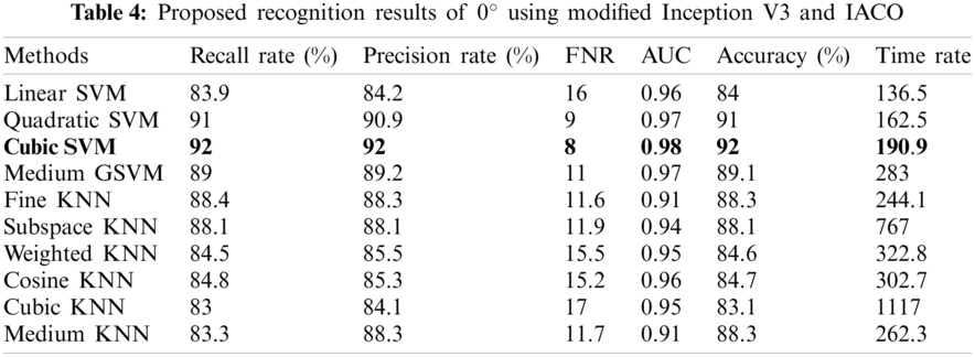
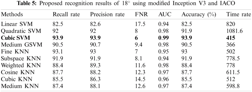
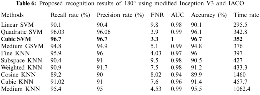
Figure 10: Confusion matrix of cubic SVM for angle 0° using modified Inception V3 and IACO

Figure 11: Confusion matrix of cubic SVM for angle 18° using modified Inception V3 and IACO

Figure 12: Confusion matrix of cubic SVM for angle 180° using modified Inception V3 and IACO

4  Conclusion and Future Work

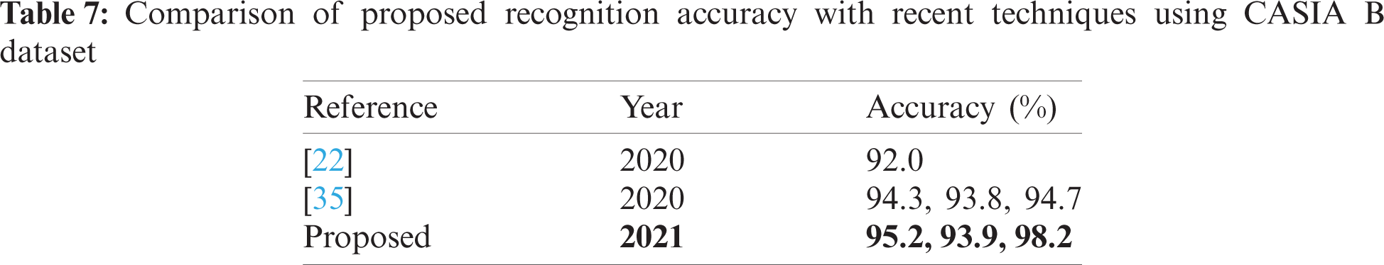
First, a brief discussion of the results section has been added to analyze the proposed framework. The results show that the proposed framework performed well on the chosen dataset. The accuracy of 0 and 180 degrees is better for modified ResNet101 and IACO, while the accuracy of 18 degrees is better for improved inceptionV3 and IACO. When compared to inceptionV3, the computational cost of improved ResNet101 and IACO is lower. Furthermore, the original computational cost of modified ResNet101 and InceptionV3 is nearly three times that of the proposed framework (applying after the IACO). Tab. 7 also includes a fair comparison with the most recent techniques. In this table, it is demonstrated that the proposed accuracy outperforms the existing techniques. Based on the results, we can conclude that the IACO aids in improving recognition accuracy while also reducing computational time. Because the accuracy of improved deep models is insufficient and falls short of recent techniques, we proposed an IACO algorithm. The choice of a deep model is the main limitation of this work because we consider both models instead of just one. In future studies, we will take this challenge into account and optimize any single deep model for HGR.

Funding Statement: This research was supported by Basic Science Research Program through the National Research Foundation of Korea (NRF) funded by the Ministry of Education (2018R1D1A1B07042967) and the Soonchunhyang University Research Fund.

Conflicts of Interest: The authors declare that they have no conflicts of interest to report regarding the present study.

References

 1.  A. Bera, D. Bhattacharjee and H. P. Shum, “Two-stage human verification using HandCAPTCHA and anti-spoofed finger biometrics with feature selection,” Expert Systems with Applications, vol. 171, pp. 114583, 2021. [Google Scholar]

 2.  M. Hassaballah and K. M. Hosny, “Recent advances in computer vision,” in Studies in Computational Intelligence, vol. 804. Cham: Springer, pp. 1–84, 2019. [Google Scholar]

 3.  S. Kadry, P. Parwekar, R. Damaševičius, A. Mehmood, J. Khan et al., “Human gait analysis for osteoarthritis prediction: A framework of deep learning and kernel extreme learning machine,” Complex and Intelligent Systems, vol. 8, pp. 1–21, 2021. [Google Scholar]

 4.  M. Sharif, M. Z. Tahir, M. Yasmim, T. Saba and U. J. Tanik, “A machine learning method with threshold based parallel feature fusion and feature selection for automated gait recognition,” Journal of Organizational and End User Computing, vol. 32, pp. 67–92, 2020. [Google Scholar]

 5.  K. Javed, S. A. Khan, T. Saba, U. Habib, J. A. Khan et al., “Human action recognition using fusion of multiview and deep features: An application to video surveillance,” Multimedia Tools and Applications, vol. 9, pp. 1–27, 2020. [Google Scholar]

 6.  Y.-D. Zhang, S. A. Khan, M. Attique, A. Rehman and S. Seo, “A resource conscious human action recognition framework using 26-layered deep convolutional neural network,” Multimedia Tools and Applications, vol. 11, pp. 1–23, 2020. [Google Scholar]

 7.  M. Hassaballah, M. A. Hameed, A. I. Awad and K. Muhammad, “A novel image steganography method for industrial internet of things security,” IEEE Transactions on Industrial Informatics, vol. 1, pp. 1–8, 2021. [Google Scholar]

 8.  H. Arshad, M. Sharif, M. Yasmin and M. Y. Javed, “Multi-level features fusion and selection for human gait recognition: An optimized framework of Bayesian model and binomial distribution,” International Journal of Machine Learning and Cybernetics, vol. 10, pp. 3601–3618, 2019. [Google Scholar]

 9.  R. Liao, S. Yu, W. An and Y. Huang, “A model-based gait recognition method with body pose and human prior knowledge,” Pattern Recognition, vol. 98, pp. 107069, 2020. [Google Scholar]

10. S. Shirke, S. Pawar and K. Shah, “Literature review: Model free human gait recognition,” in 2014 Fourth Int. Conf. on Communication Systems and Network Technologies, NY, USA, pp. 891–895, 2014. [Google Scholar]

11. X. Wang and W. Q. Yan, “Human gait recognition based on frame-by-frame gait energy images and convolutional long short-term memory,” International Journal of Neural Systems, vol. 30, pp. 1950027, 2020. [Google Scholar]

12. M. Kumar, N. Singh, R. Kumar, S. Goel and K. Kumar, “Gait recognition based on vision systems: A systematic survey,” Journal of Visual Communication and Image Representation, vol. 4, pp. 103052, 2021. [Google Scholar]

13. M. Deng, T. Fan, J. Cao, S.-Y. Fung and J. Zhang, “Human gait recognition based on deterministic learning and knowledge fusion through multiple walking views,” Journal of the Franklin Institute, vol. 357, pp. 2471–2491, 2020. [Google Scholar]

14. A. Tarun and A. Nandy, “Human gait classification using deep learning approaches,” in Proc. of Int. Conf. on Computational Intelligence and Data Engineering, NY, USA, pp. 185–199, 2021. [Google Scholar]

15. M. Sharif, T. Akram, M. Raza, T. Saba and A. Rehman, “Hand-crafted and deep convolutional neural network features fusion and selection strategy: An application to intelligent human action recognition,” Applied Soft Computing, vol. 87, pp. 105986, 2020. [Google Scholar]

16. A. Sharif, K. Javed, H. Gulfam, T. Iqbal, T. Saba et al., “Intelligent human action recognition: A framework of optimal features selection based on Euclidean distance and strong correlation,” Journal of Control Engineering and Applied Informatics, vol. 21, pp. 3–11, 2019. [Google Scholar]

17. M. S. Sarfraz, M. Alhaisoni, A. A. Albesher, S. Wang and I. Ashraf, “Stomachnet: Optimal deep learning features fusion for stomach abnormalities classification,” IEEE Access, vol. 8, pp. 197969–197981, 2020. [Google Scholar]

18. N. Hussain, A. Majid, M. Alhaisoni, S. A. C. Bukhari, S. Kadry et al., “Classification of positive COVID-19 CT scans using deep learning,” Computers, Materials and Continua, vol. 66, pp. 1–15, 2021. [Google Scholar]

19. M. Rashid, M. A. Khan, M. Alhaisoni, S.-H. Wang, S. R. Naqvi et al., “A sustainable deep learning framework for object recognition using multi-layers deep features fusion and selection,” Sustainability, vol. 12, pp. 5037, 2020. [Google Scholar]

20. A. Mehmood, S. A. Khan, M. Shaheen and T. Saba, “Prosperous human gait recognition: An end-to-end system based on pre-trained CNN features selection,” Multimedia Tools and Applications, vol. 11, pp. 1–21, 2020. [Google Scholar]

21. R. Anusha and C. Jaidhar, “Clothing invariant human gait recognition using modified local optimal oriented pattern binary descriptor,” Multimedia Tools and Applications, vol. 79, pp. 2873–2896, 2020. [Google Scholar]

22. H. Arshad, M. I. Sharif, M. Yasmin, J. M. R. Tavares, Y. D. Zhang et al., “A multilevel paradigm for deep convolutional neural network features selection with an application to human gait recognition,” Expert Systems, pp. e12541, 2020. [Google Scholar]

23. K. Sugandhi, F. F. Wahid and G. Raju, “Statistical features from frame aggregation and differences for human gait recognition,” Multimedia Tools and Applications, vol. 18, pp. 1–20, 2021. [Google Scholar]

24. S. Zheng, J. Zhang, K. Huang, R. He and T. Tan, “Robust view transformation model for gait recognition,” in 2011 18th IEEE Int. Conf. on Image Processing, NY, USA, 2011, pp. 2073–2076. [Google Scholar]

25. Y.-D. Zhang, M. Sharif and T. Akram, “Pixels to classes: Intelligent learning framework for multiclass skin lesion localization and classification,” Computers & Electrical Engineering, vol. 90, pp. 106956, 2021. [Google Scholar]

26. T. Akram, Y.-D. Zhang and M. Sharif, “Attributes based skin lesion detection and recognition: A mask RCNN and transfer learning-based deep learning framework,” Pattern Recognition Letters, vol. 143, pp. 58–66, 2021. [Google Scholar]

27. F. Emmert-Streib, Z. Yang, H. Feng, S. Tripathi and M. Dehmer, “An introductory review of deep learning for prediction models with big data,” Frontiers in Artificial Intelligence, vol. 3, pp. 4, 2020. [Google Scholar]

28. Y. Rao, L. He and J. Zhu, “A residual convolutional neural network for pan-shaprening,” in 2017 Int. Workshop on Remote Sensing with Intelligent Processing, Toranto, Canada, pp. 1–4, 2017. [Google Scholar]

29. T. Kaur and T. K. Gandhi, “Deep convolutional neural networks with transfer learning for automated brain image classification,” Machine Vision and Applications, vol. 31, pp. 1–16, 2020. [Google Scholar]

30. M. B. Tahir, K. Javed, S. Kadry, Y.-D. Zhang, T. Akram et al., “Recognition of apple leaf diseases using deep learning and variances-controlled features reduction,” Microprocessors and Microsystems, vol. 6, pp. 104027, 2021. [Google Scholar]

31. M. G. D. Dionson and P. B. El Jireh, “Inception-v3 architecture in dermatoglyphics-based temperament classification,” Philippine Social Science Journal, vol. 3, pp. 173–174, 2020. [Google Scholar]

32. T. Akram, S. Gul, A. Shahzad, M. Altaf, S. S. R. Naqvi et al., “A novel framework for rapid diagnosis of COVID-19 on computed tomography scans,” Pattern Analysis and Applications, vol. 8, pp. 1–14, 2021. [Google Scholar]

33. I. M. Nasir, M. Yasmin, J. H. Shah, M. Gabryel, R. Scherer et al., “Pearson correlation-based feature selection for document classification using balanced training,” Sensors, vol. 20, pp. 6793, 2020. [Google Scholar]

34. M. Paniri, M. B. Dowlatshahi and H. Nezamabadi-pour, “MLACO: A multi-label feature selection algorithm based on ant colony optimization,” Knowledge-Based Systems, vol. 192, pp. 105285, 2020. [Google Scholar]

35. A. Mehmood, M. A. Khan, S. A. Khan, M. Shaheen, T. Saba et al., “Prosperous human gait recognition: An end-to-end system based on pre-trained CNN features selection,” Multimedia Tools and Applications, vol. 2, pp. 1–21, 2020. [Google Scholar]

This work is licensed under a Creative Commons Attribution 4.0 International License, which permits unrestricted use, distribution, and reproduction in any medium, provided the original work is properly cited.