Computers, Materials & Continua DOI:10.32604/cmc.2022.018146
Article

Designing Bayesian New Group Chain Sampling Plan For Quality Regions

Waqar Hafeez1, Nazrina Aziz1,2,*, Zakiyah Zain1,2 and Nur Azulia Kamarudin1

1School of Quantitative of Sciences, Universiti Utara Malaysia, Sintok, 06010, Malaysia
2Institute of Strategic Industrial Decision Modelling (ISIDM), Universiti Utara Malaysia, Sintok, 06010, Malaysia
*Corresponding Author: Nazrina Aziz. Email: nazrina@uum.edu.my
Received: 26 February 2021; Accepted: 16 April 2021

Abstract: Acceptance sampling is a well-established statistical technique in quality assurance. Acceptance sampling is used to decide, acceptance or rejection of a lot based on the inspection of its random sample. Experts concur that the Bayesian approach is the best approach to make a correct decision, when historical knowledge is available. This paper suggests a Bayesian new group chain sampling plan (BNGChSP) to estimate average probability of acceptance. Binomial distribution function is used to differentiate between defective and non-defective products. Beta distribution is considered as a suitable prior distribution. Derivation is completed for the estimation of the average proportion of defectives. This study includes four quality regions namely: (i) probabilistic quality region (PQR), (ii) quality decision region (QDR), (iii) limiting quality region (LQR), and (iv) indifference quality region (IQR). The estimated values for the BNGChSP are tabulated and the inflection point values are derived, based on different combinations of design parameters including both consumer’s and producer’s risks. For comparison with the existing plan, the operating characteristic curves expose that BNGChSP is a better substitute for industrial practitioners.

Keywords: Binomial; beta distribution; consumer’s risk; producer’s risk; quality region

1  Introduction

Quality assurance is one of the most important factors for industrial production in the world. Since the last century, its applications in the manufacturing and service industries have been increasing. As the people are concerned with their critical importance in the production of manufacturing products [1]. A technique in statistical quality assurance is acceptance sampling, where based on different attributes inspection is performed on a sample of items selected from the lot under inspection. To make a decision about a lot under inspection, one option is to do a hundred percent inspection and the other is acceptance sampling. The cost and the time on inspection can be reduced by using acceptance sampling because they are directly related to sample size [2]. For example, one or few grapes can be tasted to find out whether the bunch of grapes is good or bad. It can be purchased if the selected grapes are good and if selected are bad it means the whole bunch is bad, then purchase is refused. This sampling inspection method can be used to determine whether a product is defective or non-defective. Based on their applications, a variety of acceptance sampling plans are used for inspection of products in industry. For example, in electronics manufacturing, hospital pharmacy, and food control [3–5].

Several acceptance sampling plans have been introduced over the decades. Based on single sample inspection, a single sampling plan (SSP) was proposed by Epstein et al. [6]. SSP is most famous in industrial engineering applications due to its simplicity and user-friendliness [7]. Dodge [8] developed a chain sampling plan (ChSP-1) to improve the probability of lot acceptance. Later, by considering the previous sample in SSP and a general family of chain sampling was suggested [9]. A process for attribute single sampling plan was given by Hald [10], to minimize average inspection cost. A single sampling plan was modified by using the acceptable quality limit (AQL) and limiting quality level (LQL). The Bayesian single sampling plan was considered, with weighted Poisson distribution [11,12] and Poisson distribution [13]. Latha et al. [14] used the gamma prior and proposed Bayesian chain sampling plan for construction and performance measures. Through quality regions, Nirmala et al. [15] designed a plan for Bayesian conditional repetitive group sampling.

Mughal et al. [16] assessed the design parameters for group acceptance sampling plan (GASP). GASP is evaluated in the form of group by using several testers at a time. In GASP sample size, n is divided into different groups, g based on the available number of testers r. Mughal et al. [17] developed an economic reliability GASP by using a group sampling plan for Pareto 2nd kind distribution. They used Poisson distribution for biased data theory in finding the necessary design parameters and weighted Poisson distributions. The proposed designs were found to require a shorter testing time. Later same work was applied in GChSP for a product's lifetime, following Pareto distribution of 2nd kind [18,19]. To satisfy pre-assumed design parameters at several quality levels, lot acceptance probability was obtained. Recently, Hafeez et al. [20] worked on GChSP [18] plan and introduced the idea of Bayesian in GChSP.

By considering quality variation, a plan namely Bayesian group chain sampling plan (BGChSP) for binomial distribution with beta distribution as prior was suggested [20]. It is to be noted that BGChSP used five acceptance criteria and can be improved by using more tight acceptance criteria. The main objective of this study is to update the acceptance criteria from five to four. This is more tight criteria against the defective product. Therefore, by tight acceptance criteria for a good plan both producer’s and consumer’s risks need to be minimized. The producer’s risk associated with type I error and the consumer’s risk associated with type II error. To achieve a good decision, both errors should be minimized to increase the correct decision power. With these objectives, this study is proposing a BNGChSP by considering i preceding lots. Also, this paper considers the indexed parameters to design BNGChSP, which are the producer’s risk (α) associated with an acceptable quality level (AQL) and consumer’s risk (β) associated with limiting quality level (LQL). Also for prior distribution parameters, the numerical illustrations are provided for QDR, PQR, LQR, and IQR.

2  Methodology

Operating procedure for the proposed plan is based on the following steps:

1.    Select an ideal number of g groups for each lot and assign r items to each group which is the sample size required (n=g∗r).

2.    Count the number of defectives d.

3.    If d=0 in the current sample, given that the preceding i sample has at most one defective (di≤1), accept the lot.

4.    If d=1 in the current sample, given that the preceding i sample has no defective (di=0) accept the lot, otherwise reject the lot.

5.    If d>1 in the current sample, reject the lot.

All the above steps can be summarized in a flow chart presented in Fig. 1.

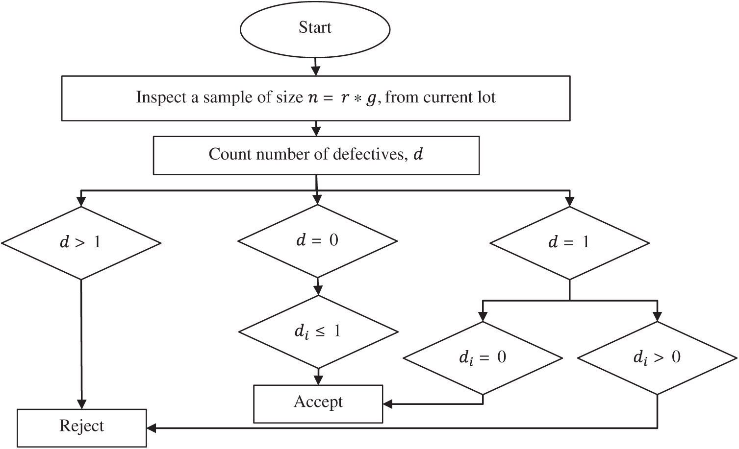
Figure 1: Operating procedure of the proposed sampling plan

For i=2, tree diagram is presented in Fig. 2, where non-defective and defective items are represented by D¯ and D respectively.

With reference to Fig. 2, for i=2, all possible outcomes that meet the acceptance criteria of NGChSP are {DD¯D¯,D¯DD¯,D¯D¯D,D¯D¯D¯}. From Fig. 2, it can be observed that the proposed sampling plan has four acceptance criteria. Let consider P0 and P1 as the probability of D¯ and D respectively, hence the probability of current lot acceptance L(p) can be written as:

L(p)=P0P0P0+3P0P0P1 (1)

L(p)=(P0)3+3P1(P0)2 (2)

and finally, for i=2 the general expression of L(p) is given by

L(P)=(P0)i+1+(i+1)(P0)iP1. (3)

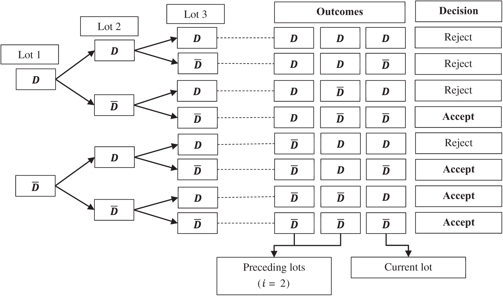
Figure 2: Tree diagram for the proposed sampling plan

Based on the properties of a binomial experiment, binomial distribution can be used to obtain the probability of zero and one defective product. It is valid because lot consists of independent and identical trials. The output from the inspection is based on two mutually exclusive outcomes either defective or non-defective. For large population with sample fraction less than 0.10, binomial distribution can be applied [21]. Hence the probability of acceptance for zero and one defective can be estimated by the binomial likelihood function.

L(c)=∑c=01(r∗gc)pc(1−p)r∗g−c, (4)

where parameter p, the probability of defectives and c is the number of defectives. For zero and one defective product, after solving Eq. (4) we get:

P0=(1−p)r∗g, (5)

P1=(r∗g)p(1−p)r∗g−1, (6)

After replacing P0 and P1 from Eqs. (5) and (6) in L(p) from Eq. (3), we get:

L(p)=(1−p)rg(i+1)+(i+1)(1−p)rgirgp(1−p)rg−1, (7)

L(p)=(1−p)rg(i+1)+(i+1)rgp(1−p)rg(i+1)−1 (8)

If the sample has a binomial distribution, then suitable prior distribution is beta distribution [22]. This means that the unknown parameter p follows beta distribution. Hence, the prior PDF for proposed sampling plan is:

f(p)=1β(s,t)ps−1(1−p)t−1 (9)

where s,t>0 are shape parameters and ss+t is the mean for beta. To estimate the average probability of acceptance, the general expression used in Bayesian is:

P¯=∫01L(p)f(p)dp (10)

After replacing Eqs. (8) and (9) in Eq. (10), we obtain:

P¯=∫01((1−p)rg(i+1)+(i+1)rgp(1−p)rg(i+1)−1)∗1β(s,t)ps−1(1−p)t−1dp (11)

P¯=1β(s,t)[β(s,rg(i+1)+t)+(i+1)rgβ(s+1,rg(i+1)+t−1)] (12)

P¯=Γ(s+t)Γ(rg(i+1)+t)Γ(t)Γ(rg(i+1)+s+t)+rg(i+1)sΓ(s+t)Γ(rg(i+1)+t−1)Γ(t)Γ(rg(i+1)+s+t) (13)

This is mixed distribution of beta and binomial, after simplify for s=1,2,3, Eq. (13) will obtain.

P¯=1−μrgμ(i+1)+1−μ+rgμ(i+1)(1−μ)(rgμ(i+1)+1−μ)(rgμ(i+1)+1−2μ); (14)

P¯=(2−μ)(2−2μ)(rgμ(i+1)+2−μ)(rgμ(i+1)+2−2μ) +2rgμ(i+1)(2−μ)(2−2μ)(rgμ(i+1)+2−μ)(rgμ(i+1)+2−2μ)(rgμ(i+1)+2−3μ); (15)

P¯=(3−μ)(3−2μ)(3−3μ)(rgμ(i+1)+3−μ)(rgμ(i+1)+3−2μ)(rgμ(i+1)+3−3μ) +3rgμ(i+1)(3−μ)(3−2μ)(3−3μ)(rgμ(i+1)+3−μ)(rgμ(i+1)+3−2μ)(rgμ(i+1)+3−3μ)(rgμ(i+1)+3−4μ). (16)

Newton’s approximation is used in Eqs. (14)–(16) to find the quality regions for BNGChSP. Where μ is used as the point of control by reducing P¯. Tab. 1 represents the average proportion of defectives, that are generated from Eqs. (14)–(16) for all the prespecified design parameters.

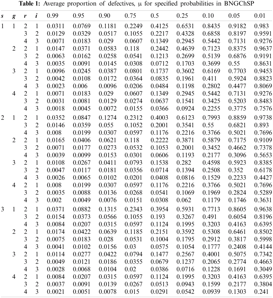
Example 1: In Tab. 1, for s=1,g=2,r=3, i=2 and P¯=0.50 the corresponding value of average proportion of defective is 0.1213 and for s=2,g=3,r=3 and i=2, the corresponding value is 0.0714. From Tab. 1, it can be noticed that as the values of s and g increase the average proportion of defective product will decrease.

2.1 Designing Sampling Plans for Given AQL and LQL

For the selection of BNGChSP, Tabs. 1 and 2 are used for specified AQL, LQL, α and β by applying the following three steps: (i) construct a plan for the given points (AQL, 1−α) and (LQL, β), then compute the required operating ratio; (ii) from Tab. 2, find the value of the operating ratio that is equal to or just less than the desired operating ratio in the desired columns for α,β; (iii) obtain the corresponding values of s,r,g and i, from Tab. 1 for the corresponding located value of the operating ratio given in Tab. 2.

Example 2: Suppose that, the value of AQL 0.0095 and LQL 0.18, with calculated operating ratio 18.9474. The approximate equal value that is closed to the calculated operating ratio in Tab. 2, is 18.542 having corresponding parametric values s=1,g=1,r=3,i=2 with α=0.10 and β=0.05. Now from Tab. 1, the corresponding values according to the above parameters for AQL is 0.0517 and LQL is 0.9591.

2.2 Designing for Quality Intervals

2.2.1 Probabilistic Quality Region

In PQR, the product is accepted with maximum probability 0.95 and minimum probability 0.05, where 0.95 corresponds to AQL (1−α) and 0.05 corresponds to LQL (β). In other words, PQR (R1) is exactly the conventional setting of AQL=μ1 and LQL=μ2. In Fig. 3 it is indicated that the PQR lies between two points μ1≤μ≤μ2.

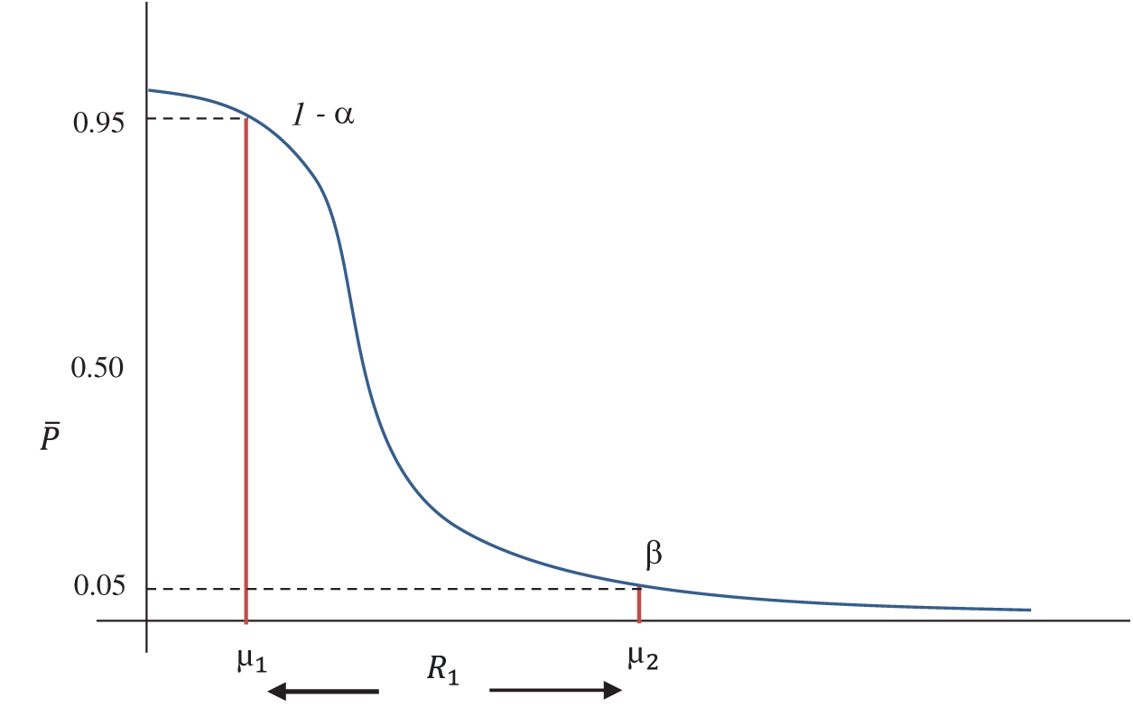
Figure 3: OC curve with pair of coordinates for PQR

This quality region considers the same values for consumer’s and producer’s risk, that is α=β=0.05 and the range of PQR is R1=μ2−μ1 provided in Tab. 3.

2.2.2 Quality Decision Region

In this quality region, the product is accepted with a maximum probability of 0.95 and the minimum probability of 0.25. Where 0.95 corresponds to AQL (1−α) and 0.25 corresponds to LQL (β). In other words, QDR (R2) is exactly the conventional setting of AQL=μ1 and LQL=μβ. In Fig. 4 it can be observed that QDR lies between two points μ1≤μ≤μβ.

Hence the values considered for consumer’s and producer’s risk are α=0.05 and β=0.25 respectively and the range of QDR is R2=μβ−μ1 given in Tab. 3.

2.2.3 Limiting Quality Region

In LQR, the product is accepted with a maximum probability of 0.75 and the minimum probability of 0.05. Where 0.75 corresponds to AQL (1−α) and 0.05 corresponds to LQL (β). In other words, LQR (R3) is exactly the conventional setting of AQL=μα and LQL=μ2. Fig. 5 defines that the LQR lies between two points μα≤μ≤μ2.

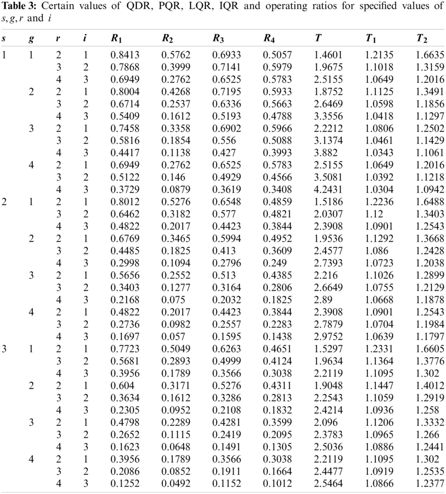
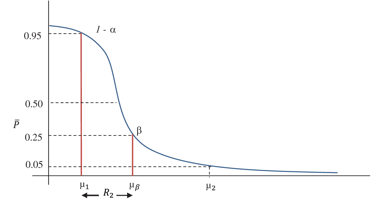
Figure 4: OC curve with pair of coordinates for QDR

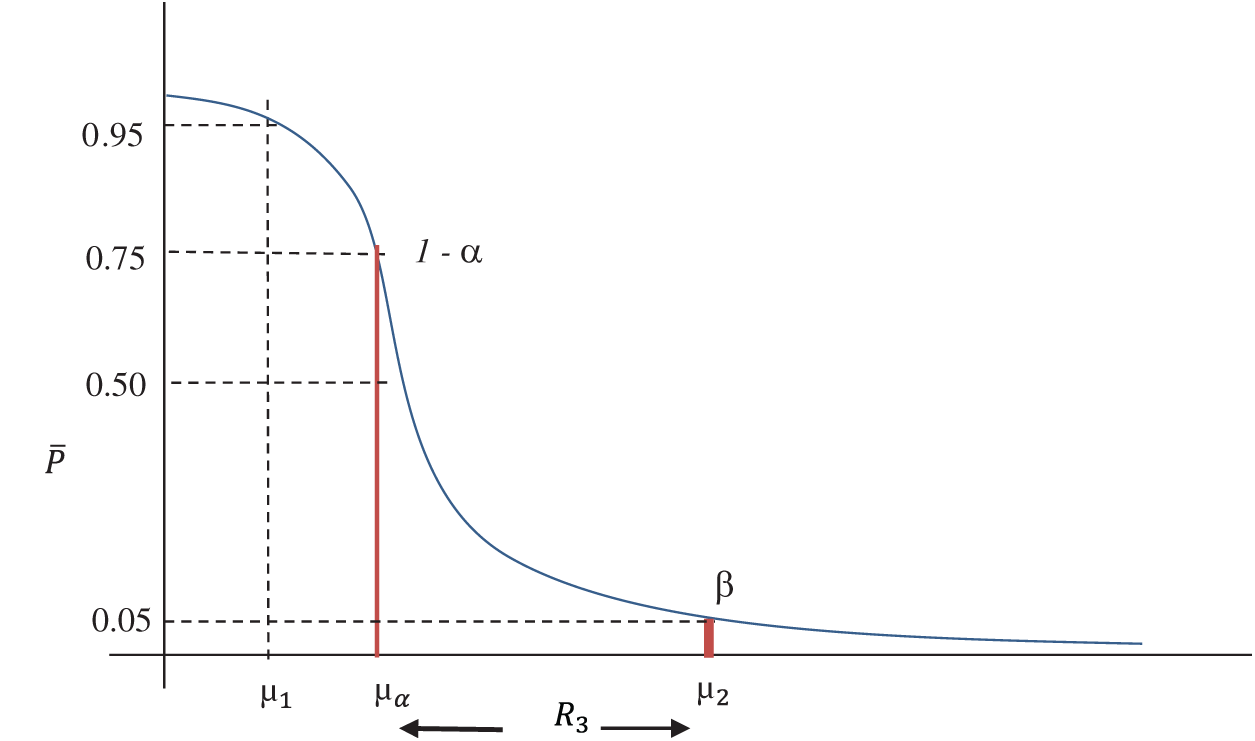
Figure 5: OC curve with pair of coordinates for LQR

In this region, the values considered for consumer’s and producer’s risk are α=0.25 and β=0.05. The range of LQR is R3=μ2−μα as given in Tab. 3.

2.2.4 Indifference Quality Region

In this quality region, the product is accepted with a maximum probability of 0.5 and the minimum probability of 0.05, where 0.5 corresponds to AQL (1−α) and 0.05 corresponds to LQL (β). In other words, IQR (R4) is exactly the conventional setting of AQL=μ∗ and LQL=μ2. Fig. 6 expresses that the IQR lies between two points μ∗≤μ≤μ2.

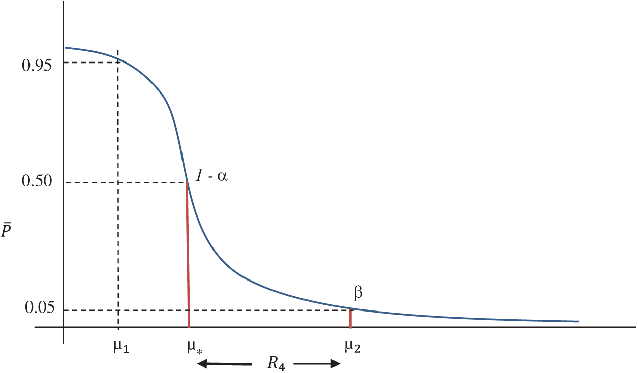
Figure 6: OC curve with pair of coordinates for IQR

In IQR the values considered for consumer’s α=0.5 and producer’s risk β=0.05 and the range is R4=μ2−μ∗ given in Tab. 3.

2.3 Selection of Sampling Plans

In Tab. 3 the range of quality regions, PQR (R1), QDR (R2), LQR (R3), IQR (R4) are presented with their corresponding design parameters s, g, r, and i. For any given values of the quality region, we can find operating ratios T=R1R2, T1=R1R3 and T2=R1R4. The value corresponding to the design parameters s, g, r and i, which is equal to or less than the specified ratio can be obtained from the columns T, T1 and T2 in Tab. 3. For this ratio, the parameters for the BNGChSP can be determined.

3  Numerical Examples

3.1 For Specified PQR and QDR

Suppose a manufacturer produces defectives within the regions of PQR 0.5% and QDR 0.25%, then R1=0.005, R2=0.0025 and the calculated operating ratio T=2.00. From Tab. 3, find the value of T that is equal to or just less than the specified ratio. The observed value is T=1.9675, with corresponding design parameters s=1, g=1, r=3 and i=2. Therefore, from Tab. 3 for this operating ratio, the range of PQR and QDR are R1=0.7868 and R2=0.3999 respectively. Hence the required design parameters for BNGChSP are s=1, g=1, r=3 and i=2, with μ1=0.0329, μβ=0.4328, and μ2=0.8197 from Tab. 1.

3.2 For Specified PQR and LQR

Let in a manufacturer defective product is found in PQR 0.5% and LQR 0.44%. Then R1=0.005, R3=0.0044 and the calculated operating ratio T1=1.136. From Tab. 3, find the value of T1 that is equal or just less than the stipulated ratio. The located value is T1=1.1292, with corresponding design parameters s=2, g=2, r=2 and i=1. Therefore, from Tab. 3, for this operating ratio the range of PQR and LQR is R1=0.6769 and R3=0.5994 respectively. Hence the required design parameters for BNGChSP are noted s=2, g=2, r=2 and i=1, with μ1=0.0406, μα=0.1180, and μ2=0.7175 from Tab. 1.

3.3 For Specified PQR and IQR

Let a producer found defective in PQR 0.5% and in IQR 0.4%, then R1=0.005, R4=0.004 and the operating ratio T2=1.25. From Tab. 3, find the value of T2 that is equal or just less than the required ratio. The value is found to be T2=1.2441, with corresponding values of design parameters are s=3, g=3, r=4 and i=3. Therefore, from Tab. 3, for this operating ratio the range of PQR and IQR are R1=0.1623 and R4=0.1305 respectively. The required design parameters for BNGChSP are s=3, g=3, r=4 and i=3, with μ1=0.0068, μ2=0.1691, and μ∗=0.0386 from Tab. 1.

4  Graphical Results and Discussion

For the specified values of s=3, r=3, i=2, and various values of g=1,2,3,4, OC curves for BNGChSP are given in Fig. 7. It can observe that as increase in the number of groups, the OC curve tends to the ideal OC curve.

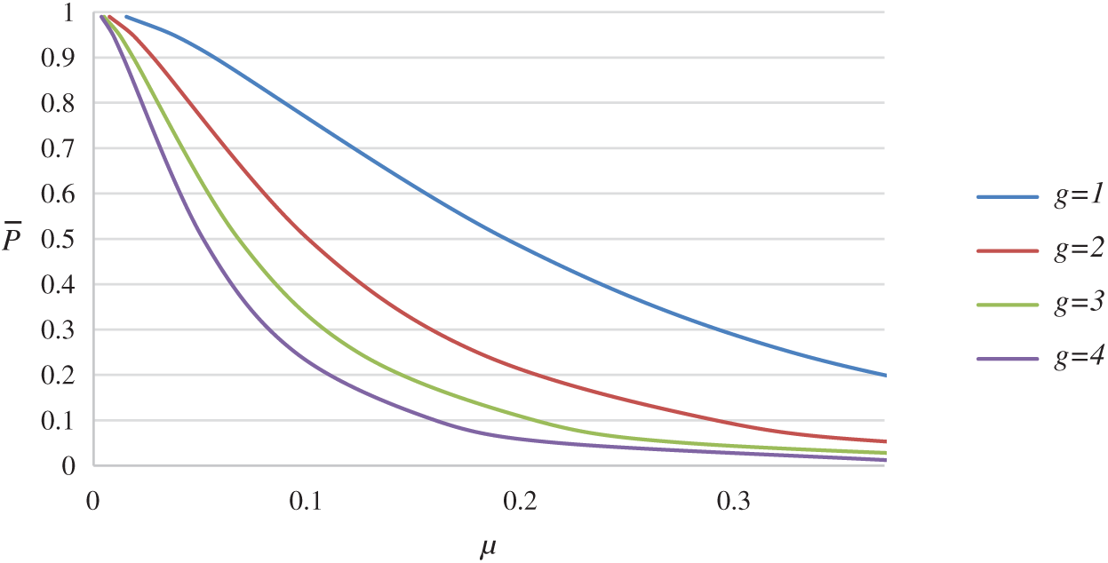
Figure 7: OC curve for BNGChSP for g=1,2,3,4

For the specified value of g=2, r=3, i=2, and different values of s=1,2,3 the OC curves for BNGChSP are presented in Fig. 8. As the value of the shape parameter increases, it can be observed that the OC curve becomes the ideal OC curve.

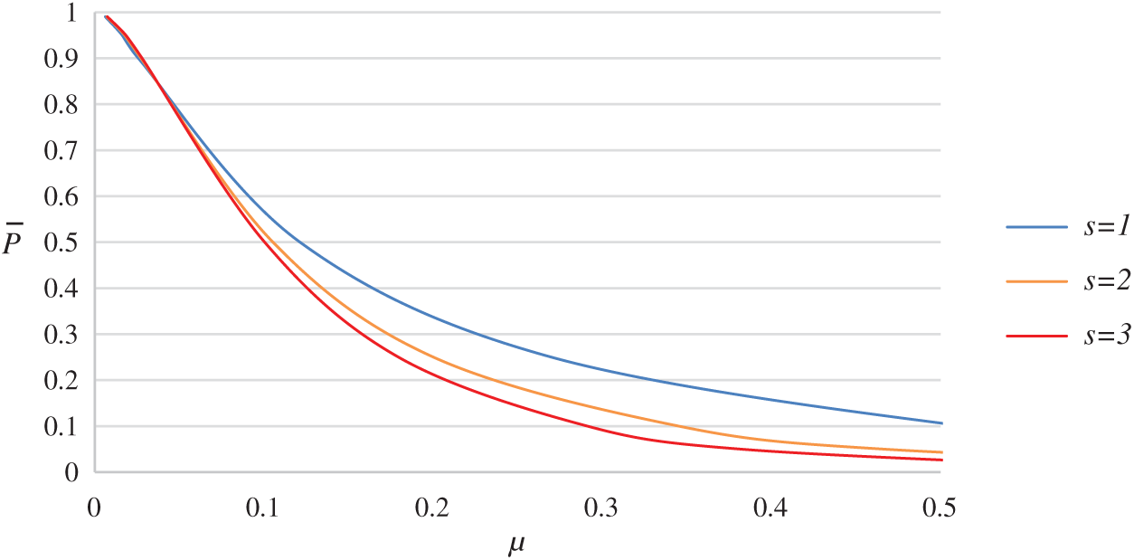
Figure 8: OC curve for BNGChSP for s=1,2 and 3

To measure the performance between proposed and existing plan. The OC curve of the proposed BNGChSP is compared with the OC curve of existing BGChSP [20]. Both plans are using binomial distribution with beta prior distribution. For the same values of design parameters s=2, g=1, r=3 and i=2, their OC curves are presented in Fig. 9.

With the average probability of acceptance P¯=0.5 and same values of other design parameters, BGChSP gives μ=0.2748, that is 27.48 percent and BNGChSP gives μ=0.20 that is 20 percent. Also, for P¯=0.9 BGChSP gives μ=0.074, that is 7.4 percent and BNGChSP gives μ=0.055, that is 5.5 percent. Based on these results, it can be concluded that BNGChSP provides a smaller proportion of defectives than the BGChSP, for the same parameter values [20]. Consequently, it can be noticed from both OC curves that BNGChSP perform better than BGChSP.

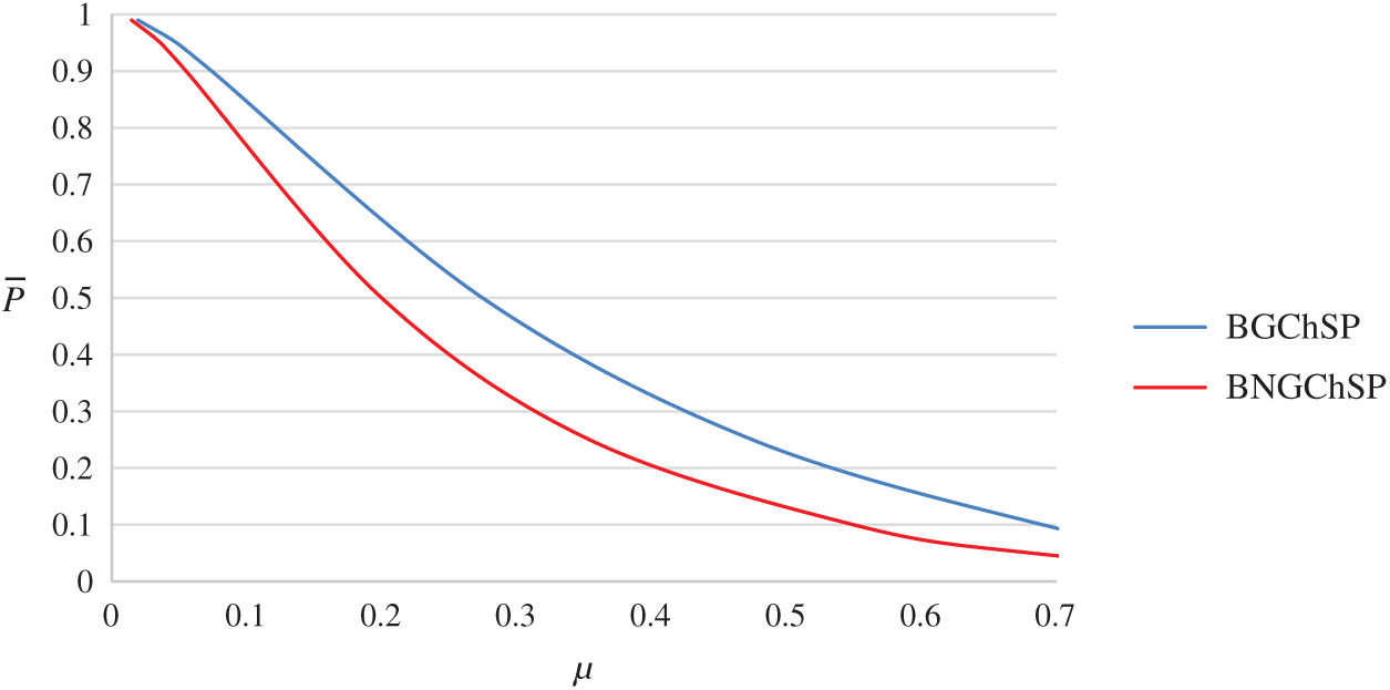
Figure 9: OC curves of BNGChSP and BGChSP

5  Conclusion

Quality interval sampling plans have wider application potential in industry to ensure that the product or process complies with a higher quality standard. Thus, quality interval sampling could be useful for outlining product quality, planning, and quality control arrangements that are ready for electronic industrial applications. For quality control practitioners, BNGChSP will be useful because it is less expensive than other plans in terms of inspection cost and time. To save the time and cost of the experiment, this research suggests the proposed plan to make the same decision as the existing plans. Many electronic components like; transport electronics systems, wireless systems, global positioning systems, and computer-supported and integrated manufacturing systems can be evaluated with proposed plan. In future many other distributions and other quality and reliability characteristics can be explored with proposed plan.

Funding Statement: This research was supported by the Ministry of Education (MOE) through Fundamental Research Grant Scheme (FRGS/1/2020/STG06/UUM/02/2), S/O Code 14884.

Conflicts of Interest: The authors declare that they have no conflicts of interest to report regarding the present study.

This work is licensed under a Creative Commons Attribution 4.0 International License, which permits unrestricted use, distribution, and reproduction in any medium, provided the original work is properly cited.