DOI:10.32604/cmc.2022.019890
| Computers, Materials & Continua DOI:10.32604/cmc.2022.019890 | |
| Article |
Two-Stage Production Planning Under Stochastic Demand: Case Study of Fertilizer Manufacturing
1Department of Industrial Engineering and Management, National Kaohsiung University of Science and Technology, Kaohsiung, 80778, Taiwan
2Sunline NP Telecommunications Co. Ltd, Kaohsiung, 80778, Taiwan
3Department of Shipping Technology, National Kaohsiung University of Science and Technology, Kaohsiung, 80778, Taiwan
4Faculty of Commerce, Van Lang University, Ho Chi Minh City, 70000, Vietnam
5Faculty of Industrial Engineering and Management, International University, Ho Chi Minh City, 70000, Vietnam
*Corresponding Author: Shao-Dong Syu. Email: shaodongsyu@gmail.com
Received: 29 April 2021; Accepted: 02 June 2021
Abstract: Agriculture is a key facilitator of economic prosperity and nourishes the huge global population. To achieve sustainable agriculture, several factors should be considered, such as increasing nutrient and water efficiency and/or improving soil health and quality. Using fertilizer is one of the fastest and easiest ways to improve the quality of nutrients inland and increase the effectiveness of crop yields. Fertilizer supplies most of the necessary nutrients for plants, and it is estimated that at least 30%–50% of crop yields is attributable to commercial fertilizer nutrient inputs. Fertilizer is always a major concern in achieving sustainable and efficient agriculture. Applying reasonable and customized fertilizers will require a significant increase in the number of formulae, involving increasing costs and the accurate forecasting of the right time to apply the suitable formulae. An alternative solution is given by two-stage production planning under stochastic demand, which divides a planning schedule into two stages. The primary stage has non-existing demand information, the inputs of which are the proportion of raw materials needed for producing fertilizer products, the cost for purchasing materials, and the production cost. The total quantity of purchased material and produced products to be used in the blending process must be defined to meet as small as possible a paid cost. At the second stage, demand appears under multiple scenarios and their respective possibilities. This stage will provide a solution for each occurring scenario to achieve the best profit. The two-stage approach is presented in this paper, the mathematical model of which is based on linear integer programming. Considering the diversity of fertilizer types, the mathematical model can advise manufacturers about which products will generate as much as profit as possible. Specifically, two objectives are taken into account. First, the paper’s thesis focuses on minimizing overall system costs, e.g., including inventory cost, purchasing cost, unit cost, and ordering cost at Stage 1. Second, the thesis pays attention to maximizing total profit based on information from customer demand, as well as being informed regarding concerns about system cost at Stage 2.
Keywords: Two-stage stochastic programming; demand uncertainty; planning; blending; fertilizer
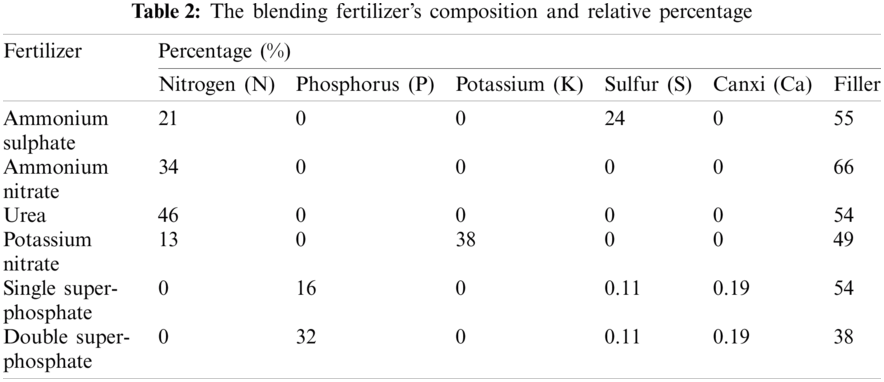
For over 40 years, the blending of solid granular materials in appropriate proportions with the purpose of producing a wide range of compound fertilizers has been well applied to fertilizer manufacturing. This process, technically called fertilizer blending (bulk blending), is one in which nutrients in a blend are mixed together physically. The three most important components needed to produce fertilizer are nitrogen (N), phosphorus (P), and potassium (K). In addition, filler material, which is added for chemical stabilization purposes and to prevent excessive fertilizer spreading causing soil “burning,” is needed. For example, the NPK formula “15-30-10” means that every 100 kilograms of this fertilizer contains 15 kg of nitrogen, 30 kg of phosphorus, and 10 kg of potassium, with 45 kg of filler.
Making an early production plan plays an important role in decreasing costs, procuring lower material costs, and meeting customer demands and requires lower bound quantities from governments with limited production capacity.
Fig. 1 shows the manufacturing planning period for the processes detailed in this paper. In the first period, Stage 1, the material purchasing price is cheap, and there is more time for manufacturing to produce products. However, the information on demand is unknown. After a certain time passes, Stage 2 begins, which is closer to the selling time, so there is more information on product demand, but the material price is more expensive than that in Stage 1. Stage 1 creates an opportunity to gain a lower cost for material and more time for producing products, but if the total quantity of purchasing material and product produced exceeded future demand, increased inventory cost will be incurred. The proposed solution, a two-stage stochastic process, uses the integer linear programming model in which the number of inputs and their quantity are treated as decision variables, and the demand is unclear information in the beginning. It is difficult to match the final demand of customers and a high inventory or holding cost is created because of excessive inventory created when demand was overestimated. However, underestimating demand leads to shortfalls and penalty costs.
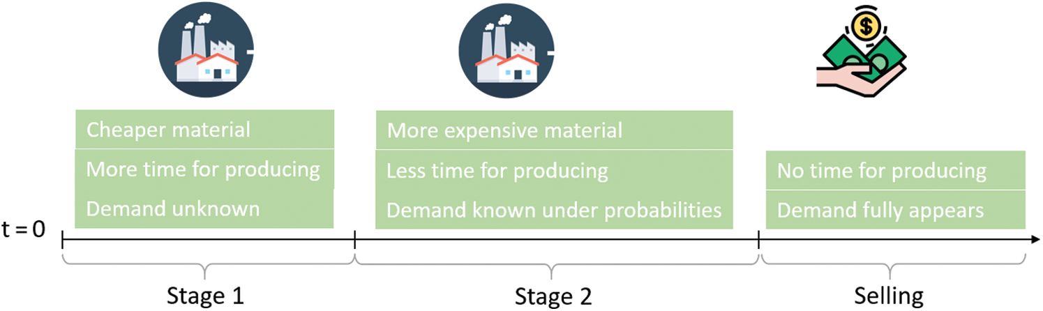
Figure 1: Planning period
In this research, the assigning of products for the production model is based on the percentage of components as developed based on the previous work of Benhamou et al. [1]. This approach has been upgraded by taking the profit from each product into account. The main objective of this paper is, for fertilizer manufacturing, to determine a solution for the best amount of purchased material due to the different price ranges in each stage, the total quantity of one-time ordering, the total products that will be produced by each blending machine, and the setting level for each machine.
Customer demand at the beginning is normally difficult to predict. Multiple optimization models have been developed over time to solve the production planning problem under changing demands [2–11]. Gupta et al. [12] suggest that demand is one of the main sources of unpredictability in any supply chain. If a supply chain fails to recognize demand fluctuations and incorporate them into planning processes, it will suffer low customer satisfaction or excessively high inventory level [13]. Uncertain demand can be modelled using probability distribution [14–18]. Gao et al. [19] approach the changing-demand planning problem with a stochastic dynamic programming model that allows delay-in-payment contracts. Huang et al. [20] propose a joint sourcing strategy framework to deal with random demand surges. The objective of the proposed framework is to minimize long-term cost while maintaining a certain target service level. Peidro et al. [21] approach a supply-chain planning problem under uncertain demand with a fuzzy mathematical programming model approach.
Weskamp et al. [22] suggest that unknown variables command attention, and propose a two-stage method. At the primary stage, the focus is on decision variables for establishing production without full information, which holds for all scenarios because restructuring this activity is costly due to the high fixed cost. In the second stage, the random probability of events exists, so then the number of materials for producing products is considered the decision variable used to minimize the total cost for manufacturing, inventory, and penalty. According to Benhamou et al. [1], a varying type of fertilizer exists to meet with customer demand. The increase in the number of fertilizer formulae leads to an increase in inventory, transportation, and production. They thus propose the reverse blending method, in which inputs are existing materials where most of the fertilizer formulas are shared like N, P, and K. Their objective is to maximize mass customization and minimize the total quantity of inputs. Emirhüseyinoğlu et al. [23] put forward that precipitation is a major uncertain factor that affects nutrient loss. They predicted nutrient reduction under stochastic precipitation rates.
Swaminathan et al. [24] present a stochastic programming model used to investigate the optimal configuration of semi-finished products and inventory levels for a multi-period planning horizon for one manufacturer. The determination of optimal differentiation points is additionally studied by Hsu et al. [25], who suggest a dynamic programming model for multiple products and unsure demand. However, their research does not consider more complex cost types, such as trans-shipment costs, and focuses only on design decisions. Liu et al. [26] introduced a two-stage mathematical optimization model to the supply-chain problem under uncertain demand. In the first stage, the production quantity of each facility of the manufacturing network and the production quantity to be transported between the network facilities are calculated. After the uncertain demand is realized and observed, the inventory size and flow of product shipped to customers are calculated in the second stage. The proposed model was implemented to solve a planning problem for a light-emitting-diode manufacturing company to demonstrate the model’s feasibility. Shi et al. [27] approach the production planning problem of a multi-product closed-loop system with uncertain demand and return with a mathematical programming model. The proposed model was applied to a real-world case study to illustrate its feasibility.
In this paper, the supply-chain planning problem under volatile demand is approached with a two-stage mathematical model with constraints on changing material price. The objectives of the proposed model are to minimize material overstock and maximize profit.
An appropriate production plan in two time periods is advanced in this paper. The outcome of the model will advise the user regarding the quantity that should be ordered at Stages 1 and 2 for each material and which blending machine is used at which level.
The mathematical model was developed based on the following assumptions.
The price of buying raw materials and ordering costs in Stage 1 is always cheaper than purchasing in Stage 2.
The length of the planning schedule in Stage 1 is 3 months, and that in Stage 2 is 5 months based on the company’s experience.
All blending machines have the same properties of all setting levels.
• The higher the setting level, the better the output and the higher the cost.
The annotations of the model are defined as follows:
• m: index of material m = 1…M
• p: index of output products p = 1…P
• r: index of price ranges r = 1…R
• e: index of scenarios e = 1…E
• j: index of ordering time j = 1…J
• b: index of blending machine b = 1…B
• i: index of setting i of blending machine i = 1…I
The parameters of the model are defined as follows:
•
•
• BigM: very large number
•
•
•
•
•
•
•
•
•
•
•
•
•
•
The decision variables of the model are defined as follows:
•
•
•
•
•
•
The auxiliary variables of the model are defined as follows:
•
•
•
The mathematical model has two objectives:
• Objective 1: Minimize total cost:
• Objective 2: Maximize profit
The constrains of the mathematical model are given below:
Constraint (1)–(2) shows that the purchased material at each time ordering is either zero or one at the one price range.
If
Constraint (3)–(8) states that each price range has its own lower bound and upper bound for the total quantity of one-time purchasing. At every ordering time belongs to price range r, the total number of purchasing must beyond lower bound and upper bound.
Range for purchasing material m at price range r
Constraint (9) focuses on total quantity purchasing material in both stages which must be smaller than the maximum usage of them in all scenarios du to prevent the unnecessary redundant.
Constraint (10)–(11) presents the number of needed material m for producing product p at stage 1 or stage 2 must be smaller than the total available of material m at that stage.
With
Constraint (12)–(13) ensures that at stage 1 and stage 2 the total time producing of all products on blending machine b must be smaller than the number of available hours of that blending machine.
Constraint (14)–(15) guarantee during production time at each stage, every blending machine will fix at only one setting level due to the high cost of changeover:
Constraint (16) defines the total income is the min of total producing product and demand from customers. If products were produced less than the demand, income will be from the total product selling. Otherwise, products were produced more than the needed, total income will come from the total demand.
Constraint (17)–(20) are binary constraints.
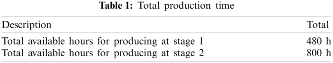
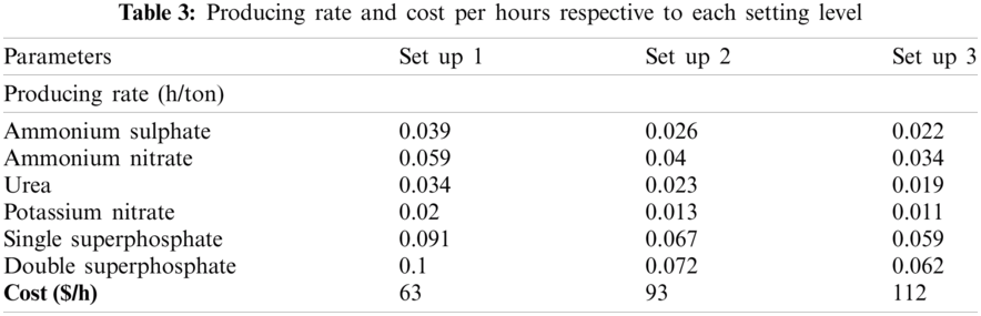
The company begins making production plans for the Fall selling season at the beginning of January annually. Stage 1 is defined as the period from the first day of January to the first day of April; Stage 2 is defined as the period between April and September. The initial manufacturing parameters are shown in Tabs. 1–3:
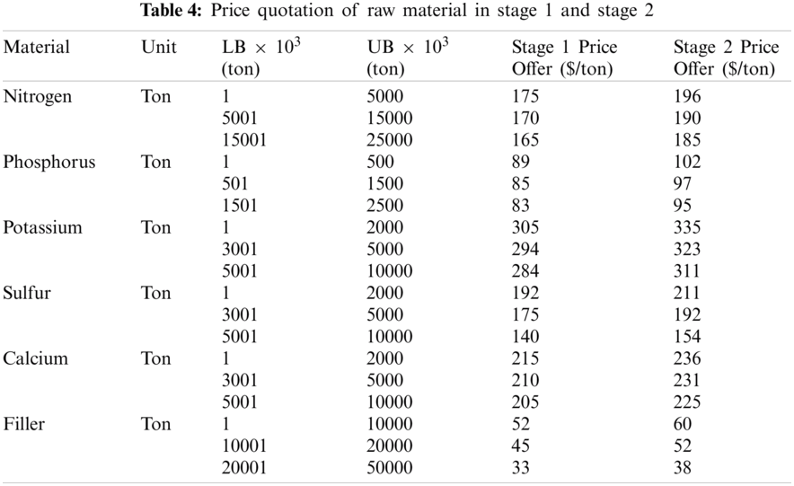
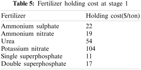
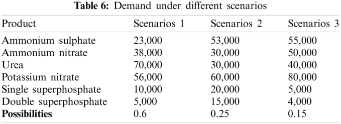
The quotations of 2 stages are shown in Tab. 4. Ordering costs at stage 1 and stage 2 are 120$ and 150$ per order, respectively. Tab. 5 enumerates the holding costs of all materials while Tab. 6 describe the demands under three different scenarios.
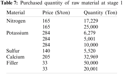
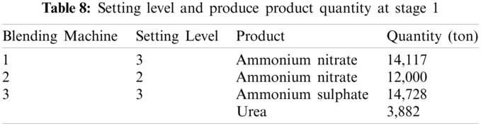
The quantity of materials that should be purchased in Stage 1 is proposed in Tab. 7. The detailed Stage 1 production plan is presented in Tab. 8.
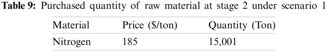
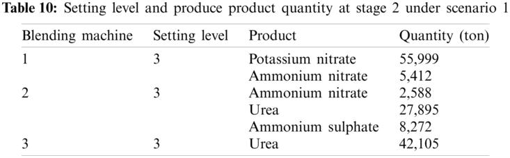
In this paper, only the results corresponding to Scenario 1, which has the highest probability of occurrence, are presented. Tabs. 9 and 10 describe the optimal Scenario 1 production plan.
Decision makers can use the results to make optimal procurement decisions. The case studied thus demonstrates the feasibility and applicability of the proposed model to real-world problems.
In this paper, a blending method and mathematical linear integer model approach are presented that comprise a decision-support tool for identifying the optimal purchased raw material and allocating the appropriate capacity for manufacturing purposes in each stage of the entire planning period for a fertilizer manufacturing planning problem. The proposed two-stage stochastic mixed-integer program was formulated to quantify total cost and managerial decision support regarding setting the levels of machines, production, and inventory. While previous research on blending fertilizer only focuses on maximizing the production of products, attention was not paid to the material or production costs. In the present study, the decision was made based on all of the costs that will affect profit. The proposed model can be improved in future research by considering other complications in the planning process such as adding output-dependent cost and price, or applying the model with rolling planning horizons.
Funding Statement: The authors received no specific funding for this study.
Conflicts of Interest: The authors declare that they have no conflicts of interest to report regarding the present study.
1. L. Benhamou, V. Giard, M. Khouloud, P. Fenies and F. Fontane, “Reverse blending: An economically efficient approach to the challenge of fertilizer mass customization,” International Journal of Production Economics, vol. 226, no. 2, pp. 107603, 2020. [Google Scholar]
2. S. Guericke, A. Koberstein, F. Schwartz and S. Voß, “A stochastic model for the implementation of postponement strategies in global distribution networks,” Decision Support Systems, vol. 53, no. 2, pp. 294–305, 2012. [Google Scholar]
3. S. Leung and W. Ng, “A stochastic programming model for production planning of perishable products with postponement,” Production Planning & Control, vol. 18, no. 3, pp. 190–202, 2007. [Google Scholar]
4. D. Peidro, J. Mula, R. Poler and F. Lario, “Quantitative models for supply chain planning under uncertainty: A review,” The International Journal of Advanced Manufacturing Technology, vol. 43, no. 3–4, pp. 400–420, 2008. [Google Scholar]
5. C. Fábián, “Handling CVaR objectives and constraints in two-stage stochastic models,” European Journal of Operational Research, vol. 191, no. 3, pp. 888–911, 2008. [Google Scholar]
6. A. Degbotse, B. T. Denton, K. Fordyce, R. J. Milne, R. Orzell et al., “IBM blends heuristics and optimization to plan its semiconductor supply chain,” Interfaces, vol. 43, no. 2, pp. 130–141, 2013. [Google Scholar]
7. B. Cole, S. Bradshaw and H. Potgieter, “An optimization methodology for a supply chain operating under any pertinent conditions of uncertainty—An application with two forms of operational uncertainty, multi-objectivity and fuzziness,” International Journal of Operational Research, vol. 23, no. 2, pp. 200, 2015. [Google Scholar]
8. F. Ciarallo, R. Akella and T. Morton, “A periodic review, production planning model with uncertain capacity and uncertain demand—Optimality of extended myopic policies,” Management Science, vol. 40, no. 3, pp. 320–332, 1994. [Google Scholar]
9. Z. Chen and B. Sarker, “Aggregate production planning with learning effect and uncertain demand,” Journal of Modelling in Management, vol. 10, no. 3, pp. 296–324, 2015. [Google Scholar]
10. J. Figueroa-García, D. Kalenatic and C. Lopez-Bello, “Multi-period mixed production planning with uncertain demands: Fuzzy and interval fuzzy sets approach,” Fuzzy Sets and Systems, vol. 206, no. 1, pp. 21–38, 2012. [Google Scholar]
11. O. Yoshida, T. Nishi, G. Zhang and J. Wu, “Design of optimal quantity discounts for multi-period bilevel production planning under uncertain demands,” Advances in Mechanical Engineering, vol. 12, no. 2, pp. 1–17, 2020. [Google Scholar]
12. A. Gupta and C. D. Maranas, “Managing demand uncertainty in supply chain planning,” Computers and Chemical Engineering, vol. 27, no. 8-9, pp. 1219–1227, 2003. [Google Scholar]
13. T. Davis, “Effective supply chain management,” Sloan Management Review, vol. 34, no. 4, pp. 35–46, 1993. [Google Scholar]
14. G. Nasiri, R. Zolfaghari and H. Davoudpour, “An integrated supply chain production-distribution planning with stochastic demands,” Computers & Industrial Engineering, vol. 77, no. 2, pp. 35–45, 2014. [Google Scholar]
15. T. Aouam and R. Uzsoy, “Zero-order production planning models with stochastic demand and workload-dependent lead times,” International Journal of Production Research, vol. 53, no. 6, pp. 1661–1679, 2014. [Google Scholar]
16. B. Kazaz, “Production planning under yield and demand uncertainty with yield-dependent cost and price,” Manufacturing & Service Operations Management, vol. 6, no. 3, pp. 209–224, 2004. [Google Scholar]
17. V. Vargas and R. Metters, “A master production scheduling procedure for stochastic demand and rolling planning horizons,” International Journal of Production Economics, vol. 132, no. 2, pp. 296–302, 2011. [Google Scholar]
18. W. Liu, W. Ma, Y. Hu, M. Jin, K. Li et al., “Production planning for stochastic manufacturing/remanufacturing system with demand substitution using a hybrid ant colony system algorithm,” Journal of Cleaner Production, vol. 213, no. 2, pp. 999–1010, 2019. [Google Scholar]
19. D. Gao, X. Zhao and W. Geng, “A delay-in-payment contract for Pareto improvement of a supply chain with stochastic demand,” Omega, vol. 49, no. 3, pp. 60–68, 2014. [Google Scholar]
20. L. Huang, J. S. Song and J. Tong, “Supply chain planning for random demand surges: Reactive capacity and safety stock,” Manufacturing & Service Operations Management, vol. 18, no. 4, pp. 509–524, 2016. [Google Scholar]
21. D. Peidro, J. Mula, R. Poler and J. L. Verdegay, “Fuzzy optimization for supply chain planning under supply, demand and process uncertainties,” Fuzzy Sets and Systems, vol. 160, no. 18, pp. 2640–2657, 2009. [Google Scholar]
22. C. Weskamp, A. Koberstein, F. Schwartz, L. Suhl and S. Voß, “A two-stage stochastic programming approach for identifying optimal postponement strategies in supply chains with uncertain demand,” Omega, vol. 83, no. 4, pp. 123–138, 2019. [Google Scholar]
23. G. Emirhüseyinoğlu and S. Ryan, “Land use optimization for nutrient reduction under stochastic precipitation rates,” Environmental Modelling & Software, vol. 123, pp. 104527, 2020. [Google Scholar]
24. J. Swaminathan and S. Tayur, “Stochastic programming models for managing product variety,” International Series in Operations Research & Management Science, vol. 17, pp. 585–622, 1999. [Google Scholar]
25. H. Hsu and W. Wang, “Dynamic programming for delayed product differentiation,” European Journal of Operational Research, vol. 156, no. 1, pp. 183–193, 2004. [Google Scholar]
26. Y. Liu, Y. Chen and G. Yang, “Developing multi-objective equilibrium optimization method for sustainable uncertain supply chain planning problems,” IEEE Transactions on Fuzzy Systems, vol. 27, no. 5, pp. 1037–1051, 2019. [Google Scholar]
27. J. Shi, G. Zhang and J. Sha, “Optimal production planning for a multi-product closed loop system with uncertain demand and return,” Computers & Operations Research, vol. 38, no. 3, pp. 641–650, 2011. [Google Scholar]
 | This work is licensed under a Creative Commons Attribution 4.0 International License, which permits unrestricted use, distribution, and reproduction in any medium, provided the original work is properly cited. |