Computers, Materials & Continua DOI:10.32604/cmc.2022.019685
Article

An Artificial Intelligence Approach for Solving Stochastic Transportation Problems

Prachi Agrawal1, Khalid Alnowibet2, Talari Ganesh1, Adel F. Alrasheedi2, Hijaz Ahmad3 and Ali Wagdy Mohamed4,5,*

1Department of Mathematics and Scientific Computing, National Institute of Technology Hamirpur, Himachal Pradesh, 177005, India
2Statistics and Operations Research Department, College of Science, King Saud University, Riyadh, 11451, Kingdom of Saudi Arabia
3Section of Mathematics, International Telematic University Uninettuno, Roma, 00186, Italy
4Operations Research Department, Faculty of Graduate Studies for Statistical Research, Cairo University, Giza, 12613, Egypt
5Wireless Intelligent Networks Center (WINC), School of Engineering and Applied Sciences, Nile University, Giza, Egypt
*Corresponding Author: Ali Wagdy Mohamed. Email: aliwagdy@gmail.com
Received: 22 April 2021; Accepted: 25 May 2021

Abstract: Recent years witness a great deal of interest in artificial intelligence (AI) tools in the area of optimization. AI has developed a large number of tools to solve the most difficult search-and-optimization problems in computer science and operations research. Indeed, metaheuristic-based algorithms are a sub-field of AI. This study presents the use of the metaheuristic algorithm, that is, water cycle algorithm (WCA), in the transportation problem. A stochastic transportation problem is considered in which the parameters supply and demand are considered as random variables that follow the Weibull distribution. Since the parameters are stochastic, the corresponding constraints are probabilistic. They are converted into deterministic constraints using the stochastic programming approach. In this study, we propose evolutionary algorithms to handle the difficulties of the complex high-dimensional optimization problems. WCA is influenced by the water cycle process of how streams and rivers flow toward the sea (optimal solution). WCA is applied to the stochastic transportation problem, and obtained results are compared with that of the new metaheuristic optimization algorithm, namely the neural network algorithm which is inspired by the biological nervous system. It is concluded that WCA presents better results when compared with the neural network algorithm.

Keywords: Artificial intelligence; metaheuristic algorithm; stochastic programming; transportation problem; water cycle algorithm; weibull distribution

1  Introduction

The issue related to transportation, which is a basic necessity of society, is called a transportation problem. The transportation problem distributes homogeneous products from different origins to different destinations. It mainly consists of three parameters: the available amount of products at origins, the required amount of products at destinations, and the transportation cost from origins to destinations. The main objective is to minimize the transportation cost based on the availability and the requirement of the product.

Kantorovich’s [1] obtained a solution for the transportation problem through his seminal work; however, Hitchcock [2] gave a constructive method for the same. Arsham et al. [3] proposed a linear programming approach to solve the same issue using the simplex algorithm.

Owing to lack of information or inaccurate data, the parameters price and demand of the product may be treated as random variables. Such transportation problems, where the pivotal parameters like demand and price are uncertain and where there is a need for mathematical programming that optimizes the uncertainty, are usually termed as “stochastic transportation problems” [4]. This is applicable to many areas including but not limited to population management, transportation, agriculture, finance ranger service, to name a few.

Over the years, the optimization of parameters in stochastic programming (SP) is focused on right side vectors in such a way that these have a certain probability distribution. Few research works in this line were by Barik et al. [5], Matiy et al. [6], Agrawal et al. [7], and Mahapatra et al. [8]. In these studies, the parameters are estimated using Pareto, Logistic, and Normal random variables. Several researchers contributed finding the solution for multichoice SP: Maity et al. [9] suggested a utility function to obtain the optimum solution, Agrawal et al. [10] worked on a nonlinear approach to have feasible and optimal values, and Roy [11,12] proposed Lagrange’s interpolation for having optimal values of multichoice parameters and also solutions in the case of stochastic supply. Mahapatra et al. [13] solved a multichoice stochastic transportation problem in which the parameters follow extreme value distribution.

However, for handling complex SP problems and having a convergence, algorithms that help in iterating the parameter values of SP and finding out the optimal solution are highly required. This has grabbed the attention of many researchers, and several works have come out on this platform too, some notable contributions of which were: genetic algorithm (GA) [14], particle swarm optimization [15], ant colony optimization [16], and differential evolution optimization [17]. Dutta et al. [18] solved a fuzzy stochastic transportation problem using GA. Vignaux et al. [19] adopted the GA to understand its utility in solving the linear transportation problem. Cao [20] solved the transportation problem with the branch and bound method, and later on, Cao et al. [21] obtained the solution of transportation with the tabu search algorithm. Later, Eskandar et al. [22] developed a novel approach to address these complex situations by building a metaheuristic algorithm called water cycle algorithm (WCA) and it is also shown that WCA works better than other metaheuristic algorithms. Furthermore, Sadollah et al. [23], Ghaffarzadeh [24], and Sadollah et al. [25] worked on WCA and applied it to enhance the parameters of a power framework stabilizer and used it to solve multi-objective optimization problems. In the recent past, Sadollah et al. [26] proposed an algorithm based on biological neural networks, named neural network algorithm (NNA), to deal with constrained optimization problems.

The main purpose of this study is to apply WCA to the stochastic transportation problem and find the optimal transportation plan of the problem. In this study, the stochastic transportation problem is considered, in which the parameters supply and demand are considered as random variables, which follow the Weibull distribution [27]. Therefore, the stochastic constraints are converted into deterministic using SP, and WCA is applied to the deterministic transportation problem. The obtained results of the case study are compared with NNA.

The paper is organized as follows. The mathematical model of the stochastic transportation problem is given in Section 2 and the methodology used to solve the stochastic transportation problem is presented in Section 3. The metaheuristic algorithm WCA is given in Section 4. To understand the methodology, the case study is presented in Section 5 and their results and conclusions are given in Sections 6 and 7, respectively.

2  Problem Specification

This section contains the introduction and mathematical model of the stochastic transportation problem. Assume that there are p and q number of supply and destination locations, respectively. Wt, Rs denote the availability of the product at the, supply locations and the requirement of the product at the , destination locations. These parameters are stochastic, are considered to follow Weibull distribution, and their corresponding constraints are probabilistic. Also cts is the transportation cost from tth supply locations to the sth destination locations. In particular, c13 describes the transportation cost from the first supply location to the third destination location. The main aim is to find the number of units xts (decision variables) of the homogeneous product that is shipped from the tth supply locations to the sth destination locations. The mathematical model of the stochastic transportation problem is written as

minZ=∑t=1p⁡∑s=1q⁡ctsxts(1)

subject to

P(∑s=1q⁡xts≤Wt)≥ηt,t=1,2,…,p,(2)

P(∑t=1p⁡xts≤Rs)≥δs,s=1,2,…,q,(3)

xts≥0,t=1,2,…,p,s=1,2,…,q.(4)

Eq. (1) represents the objective function, and (2) and (3) are the constraints of supply and destination which are probabilistic with a specified probability, respectively.

3  Methodology

This section describes the methodology applied to the stochastic transportation problem to find the optimal solution. The problem contains probabilistic constraints, and to convert them into deterministic, SP is used and then metaheuristic algorithm WCA is applied to the deterministic problem. The description of the methodology is presented in the following sections.

3.1 Transformation of Stochastic Constraints

Theorem 1. Let Wt, t=1,2,…,p, are independent Weibull random variables with αt,βt, and γt being the location, scale, and shape parameters, respectively. Then the probabilistic constraint (2) is converted into deterministic as

Proof: Consider tth(t=1,2,…,q) supply constraint:

It can be rewritten as

P(Wt≤∑s=1q⁡xts)≥1−ηt.(5)

Since Wt(t=1,2,…,q) are random variables that follow Weibull distribution, the probability density function of Wt is given by

where Wt≥αt,αt∈R,η>0,andγt>0.

Eq. (5) is rewritten as

which implies that

∫αt∑s=1qxts⁡γtβt(Wt−αtβt)γt−1e−[(Wt−αtβt)γt]d(Wt)≤1−ηt.(6)

To solve this integral, let (Wt−αtβt)γt=y. Therefore, (6) is rewritten as

This implies that

Taking logarithm on both sides, we obtain

This implies that

On simplifying, we obtain

∑s=1q⁡xts≤αt+βt[−ln⁡(ηt)]1/γt,t=1,2,…,p.(7)

Eq. (7) is the deterministic constraint of the supply probabilistic constraint (2).

Theorem 2. Let Rs, s=1,2,…,q, are independent Weibull random variables with αs¯,βs¯,andγs¯ being the location, scale, and shape parameters, respectively. Then the probabilistic constraint (3) is converted into deterministic as

∑t=1p⁡xts≥αs¯+βs¯[−ln⁡(1−δs)]1/γs,s=1,2,…,q.(8)

Proof: The proof follows the same procedure as in Theorem 1, and, therefore, we omit it.

Eq. (8) is the deterministic constraint of the demand probabilistic constraint (3).

3.2 The Mathematical Model

Using SP, the deterministic mathematical model of the stochastic transportation problem is written as follows:

s.t.

4  Water Cycle Algorithm

The thought behind WCA is invigorated from nature, based on the perception of the water cycle, and how rivers and streams stream downhill toward the sea in reality. A river, or a stream, is shaped at whatever point water moves downhill, starting with one point and then onto the next. This shows that most rivers are framed high up in the mountains, where snow or ice sheets liquefy. The rivers consistently stream downhill. On their downhill adventure and at the end winding up to the sea, water is gathered from the downpour and different streams. Water in streams and lakes evaporates to create mists which at that point consolidates in the colder air, discharging the water back to the earth as downpour or precipitation.

4.1 Initial Solution Generation

The population-based metaheuristic algorithm WCA begins with the initial population, called raindrops. A raindrop represents an array of 1×nVar, where nVar is the dimension of the optimization problem. The 1×nVar array represents the decision variables, which is defined as follows:

In the array, the best raindrop is picked as the sea, and at that point, various great raindrops are picked as the river, and the remainder of the raindrops are considered as streams which flow to the rivers and sea. A candidate solution represents a matrix of raindrops of size nPop×nVar which is generated randomly. Hence, the matrix X is written as

Each of the decision variables (kx1,kx2,…,kxnVar) is represented as floating-point numbers, but all the decision variables have to be non-negative. NSR (user-defined parameter) represents the summation of the number of rivers and sea (single value), as shown in the following equation:

NSR=Numberofrivers+1(9)

and the remainder of the population is calculated from

NRD=nPop−NSR.(10)

In (9), 1 represents the sea value, and in (10), NRD denote the number of raindrops.

4.2 Evaluation of Fitness

The objective function (cost function) is evaluated at the raindrops kx1,kx2,…,kxnVar, k=1,2,…,nPop:

where nPop and nVar are the number of raindrops and the number of decision variables, respectively.

4.3 Designate Streams to Rivers and Sea

To assign/appoint raindrops to the rivers and sea relying on the power of the flow, the accompanying equation is given in which NSn denotes the numbers of streams that flow to the specific rivers or sea:

NSn=round[Objectiven∑i=1NSR⁡Objectivei×NRD],n=1,2,…,NSR(11)

4.4 Formation of Rivers and Streams

In WCA, the streams are made from the raindrops, which join with others to form new rivers. Likewise, a portion of the streams straightforwardly moves to the sea. Every river and every stream end up in the sea. With distance, a stream moves toward the river along the interfacing line between them. The distance is chosen randomly, which is given as

X∈(0,v×d),1≤v≤2,(12)

where d is the current distance between the stream and the river. The value of X depends on the random number between 0 and v×d.

Therefore, the new streams and rivers are written as

where kXSt and kXR are the position of the stream and the river at kth iteration, respectively, and the rand is a uniformly distributed random number between 0 and 1. The position of the river and streams will be interchanged if the solution obtained by the stream is better than its connecting river. The same will be applied to rivers and sea.

4.5 Evaporation

The main part of the algorithm is based on evaporation, which prevents the algorithm from rapid convergence. In the water cycle, water evaporates from rivers and lakes, while plants give off water during photosynthesis. The evaporated water is carried into the atmosphere to clouds which then condenses in the colder atmosphere, releasing the water back to the earth in the form of rain. The rain creates the new streams, and the new streams flow to the rivers which in turn flow to the sea. In WCA, the vanishing procedure causes the seawater to dissipate, as waterways/streams stream to the sea. This idea is utilized to abstain from getting caught in local optima. The drizzling procedure is connected for which new raindrop structure streams in various areas. For indicating the new areas of the recently shaped streams, the accompanying condition is utilized:

newXSt=Lb+rand×(Ub−Lb),(13)

where Lb and Ub are the lower and upper bounds of the decision variables, respectively, which is defined in the problem. Again, the best newly formed raindrop is considered as a river flowing to the sea.

5  Case Study

A numerical example is considered for a better understanding of the proposed methodology, in which supply and demand follow the Weibull distribution. It presents a case study of tea transportation, which contains three supply locations and four destination locations in India. Tea is transported from the bottom of hill areas to different areas. It is transported at Palampur, The tea capital of North India, in Kangra district, Himachal Pradesh, India, from Bir, Thakurdwara, and Dharamsala, to four destination locations of Delhi, Punjab, Rajasthan, and Uttar Pradesh. The cost of transporting one unit (50 kg) from supply location to destination locations is considered. The main aim is to minimize the total transportation cost for availability and the requirement of the tea. The corresponding objective function and the related data are presented.

Tab. 1 presents the data relating to Weibull distribution with three known parameters of supply and demand.

First, using the data, the mathematical model of the stochastic transportation problem involving the Weibull distribution is formulated. The objective function is given in the following form subject to probabilistic constraints. The probabilistic model is converted into a deterministic model using the transformation technique and then solved by WCA and NNA.

minZ=10x11+10x12+20x13+11x14+12x21+7x22+9x23+20x24+10x31+14x32+16x33+18x34(14)

s.t.

6  Results and Discussion

A case study based on the stochastic transportation problem involving Weibull distribution is presented in Section 5, and using SP, the problem is converted into its deterministic form. WCA is applied to obtain the solution of the problem that contains 12 decision variables and 19 constraints. The problem is solved using MATLAB software, and the codes were run on a computer with Intel (R) Core (TM)2 Quad, a CPU clock of 2.33 GHz with 4.00 GB RAM. Tab. 2 presents the values of the parameters used in WCA.

For each run, the initial candidate solution was generated randomly within the boundaries using a uniform probability distribution. Tolerance, which is defined by the user, is ϵ = 2.22E − 16$ and the maximum number of iterations was set to 1000. Similarly, the number of the total population and the maximum number of iterations for the NNA were set as reported in the WCA. Twenty-five independent runs were performed for both the algorithms and the obtained results are noted throughout the process. It can be observed from the obtained results that WCA has the optimal (minimum) objective value in the 20th run and has the worst objective value in the fifth run. The best (optimal), average, and the worst objective values are shown in Tab. 3, which depicts that the WCA presents better solutions when compared to NNA.

Fig. 1 shows that WCA and NNA are comparable: using WCA, the obtained value is 22495.384 which occurs at the 77th iteration, whereas using NNA, the objective value is 23534.583 which occurs at the 387th iteration.

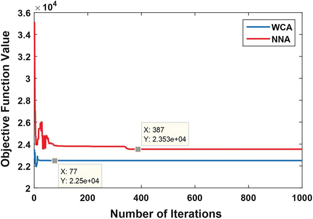
Figure 1: The convergence graph for solving the stochastic transportation problem at the third run using WCA and NNA

The convergence graph of WCA and NNA at the optimal solution is presented in Fig. 2. It can be observed from the figure that the convergence of WCA is faster than that of NNA. WCA is stable after 203 iterations, whereas NNA is stable after 569 iterations.

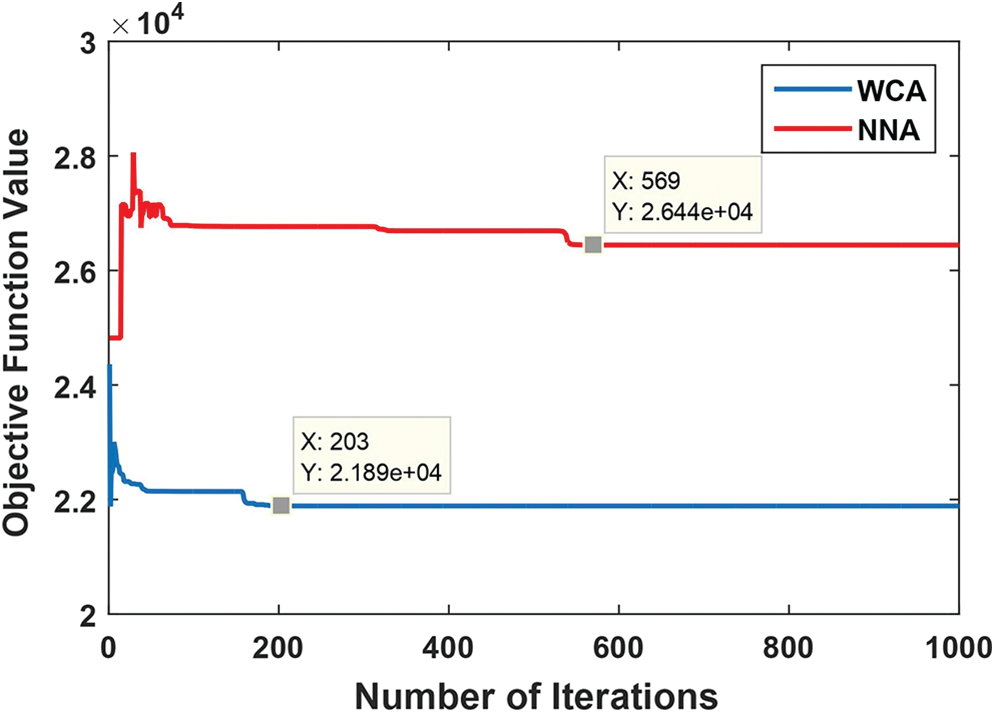
Figure 2: The convergence graph of the optimal solution obtained by WCA and NNA of the stochastic transportation problem

Fig. 3 illustrates the convergence graph of WCA and NNA at the worst solution. The convergence of WCA is much stable than that of NNA. WCA converges after 64 iterations, whereas NNA converges after 500 iterations.

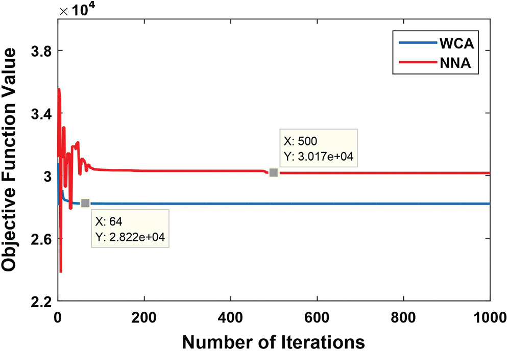
Figure 3: The convergence graph of the optimal solution obtained by WCA and NNA of the stochastic transportation problem

Also, for each run, the elapsed time is calculated using WCA and NNA, which is shown in Fig. 4.

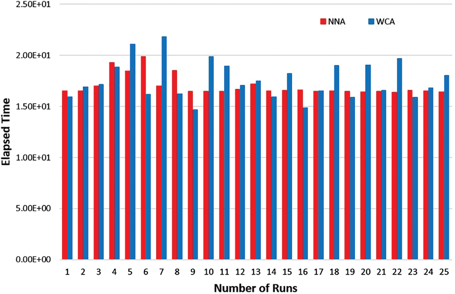
Figure 4: The elapsed time taken by WCA and NNA at each run

It is concluded that for solving transportation problem, the decision-maker opt for the best solution, which means that the number of units that are transferred from different supply locations to different destination locations are x11=62.22365,x12=0.0205 (∼0),x13=30.98294,x14=461.7318,x21=1.339141,x22=118.9762,x23=501.3241,x24=34.68913,x31=267.6457,x32=312.9103,x33=0,x34=136.3857, and the total transportation cost is Rs. 21887.897.

7  Conclusions

In this study, the stochastic transportation problem is considered in which supply and demand are Weibull random variables. This work incorporates the WCA algorithm into the stochastic transportation problem to obtain the optimal solution. Since the transportation problem contains a large number of constraints, the constraints are handled using Deb’s constraint handling techniques. The problem is also solved by a metaheuristic algorithm NNA and the obtained results are compared. All the constraints are handled in WCA and NNA. The results show that WCA gives significant results when compared to NNA. As a future scope, WCA can be applied to the multi-objective stochastic transportation problem to find the optimal solution that can satisfy all the objectives.

Acknowledgement: The authors extend their appreciation to the Deanship of Scientific Research at King Saud University for funding this work through research group number RG-1436-040.

Funding Statement: This work was funded by the Deanship of Scientific Research at King Saud University through research Group Number RG-1436-040.

Conflicts of Interest: The authors declare that they have no conflicts of interest to report regarding the present study.

References

 1.  L. V. Kantorovich, “Mathematical methods in the organization and planning of production,” Management Science, vol. 6, no. 4, pp. 366–422, 1960. [Google Scholar]

 2.  F. L. Hitchcock, “The distribution of a product from several sources to numerous localities,” Journal of Mathematical Physics, vol. 20, no. 1–4, pp. 224–230, 1941. [Google Scholar]

 3.  H. Arsham and A. B. Kahn, “A simplex-type algorithm for general transportation problems: An alternative to stepping-stone,” Journal of Operational Research Society, vol. 40, no. 6, pp. 581–590, 1989. [Google Scholar]

 4.  A. C. Williams, “A stochastic transportation problem,” Operations Research, vol. 11, no. 5, pp. 759–770, 1963. [Google Scholar]

 5.  S. K. Barik, M. P. Biswal and D. Chakravarty, “Stochastic programming problems involving pareto distribution,” Journal of Interdisciplinary Mathematics, vol. 14, no. 1, pp. 40–56, 2011. [Google Scholar]

 6.  G. Maity and S. Roy Kumar, “Solving a multi-objective transportation problem with nonlinear cost and multi-choice demand,” International Journal of Industrial Engineering and Management Science, vol. 11, no. 1, pp. 62–70, 2016. [Google Scholar]

 7.  P. Agrawal and T. Ganesh, “Multi-choice stochastic transportation problem involving logistic distribution,” Advances and Applications in Mathematical Sciences, vol. 18, no. 1, pp. 45–58, 2018. [Google Scholar]

 8.  D. R. Mahapatra, S. K. Roy and M. P. Biswal, “Stochastic based on multi-objective transportation problems involving normal randomness,” Advanced Modeling and Optimization, vol. 12, no. 2, pp. 205–223, 2010. [Google Scholar]

 9.  G. Maity and S. K. Roy, “Solving multi-choice multi-objective transportation problem: A utility function approach,” Journal of Uncertainty Analysis and Applications, vol. 2, no. 1, pp. 1–20, 2014. [Google Scholar]

10. P. Agrawal and T. Ganesh, “Solving transportation problem with stochastic demand and non-linear multi-choice cost,” AIP Conference Proceedings, vol. 2134, pp. 60002, 2019. [Google Scholar]

11. S. K. Roy, “Lagrange’s interpolating polynomial approach to solve multi-choice transportation problem,” International Journal of Applied and Computational Mathematics, vol. 1, no. 4, pp. 639–649, 2015. [Google Scholar]

12. S. K. Roy, “Transportation problem with multi-choice cost and demand and stochastic supply,” Journal of the Operations Research Society of China, vol. 4, no. 2, pp. 193–204, 2016. [Google Scholar]

13. D. R. Mahapatra, S. K. Roy and M. P. Biswal, “Multi-choice stochastic transportation problem involving extreme value distribution,” Applied Mathematical Modelling, vol. 37, no. 4, pp. 2230–2240, 2013. [Google Scholar]

14. D. Goldberg, Genetic Algorithms in Search, Optimization and Machine Learning Reading. MA: Addison-Wesley, 1989. [Google Scholar]

15. Q. He and L. Wang, “An effective co-evolutionary particle swarm optimization for engineering optimization problems,” Engineering Applications of Artificial Intelligence, vol. 20, pp. 89–99, 2006. [Google Scholar]

16. M. Dorigo and G. Di Caro, “Ant colony optimization: A new meta-heuristic”, in Proc. of the 1999 Congress on Evolutionary Computation-CEC99 (Cat. No. 99TH8406IEEE, vol. 2, Washington, DC, USA, pp. 1470–1477, 1999. [Google Scholar]

17. F. Z. Huang, L. Wang and Q. He, “An effective co-evolutionary differential evolution for constrained optimization,” Applied Mathematics and Computation, vol. 186, no. 1, pp. 340–56, 2007. [Google Scholar]

18. S. Dutta, S. Acharya and R. Mishra, “Genetic algorithm based fuzzy stochastic transportation programming problem with continuous random variables,” Opsearch, vol. 53, no. 4, pp. 835–872, 2016. [Google Scholar]

19. G. A. Vignaux and Z. Michalewicz, “A genetic algorithm for the linear transportation problem,” IEEE Transactions on Systems, Man and Cybernetics, vol. 21, no. 2, pp. 445–452, 1991. [Google Scholar]

20. B. Cao, “Transportation problem with nonlinear side constraints a branch and bound approach,” Operational Research, vol. 36, no. 2, pp. 185–197, 1992. [Google Scholar]

21. B. Cao and G. Uebe, “Solving transportation problems with nonlinear side constraints with tabu search,” Computers & Operations Research, vol. 22, no. 6, pp. 593–603, 1995. [Google Scholar]

22. H. Eskandar, A. Sadollah, A. Bahreininejad and M. Hamdi “Water cycle algorithm—A novel metaheuristic optimization method for solving constrained engineering optimization problems,” Computers & Structures, vol. 110–111, pp. 151–166, 2012. [Google Scholar]

23. A. Sadollah, H. Eskandar, A. Bahreininejad and J. H. Kim, “Water cycle algorithm with evaporation rate for solving constrained and unconstrained optimization problems,” Applied Soft Computing, vol. 30, pp. 58–71, 2015. [Google Scholar]

24. N. Ghaffarzadeh, “Water cycle algorithm based power system stabilizer robust design for power systems,” Journal of Electrical Engineering, vol. 66, no. 2, pp. 91–96, 2015. [Google Scholar]

25. A. Sadollah, H. Eskandar and J. H. Kim, “Water cycle algorithm for solving constrained multi-objective optimization problems,” Applied Soft Computing, vol. 27, pp. 279–298, 2015. [Google Scholar]

26. A. Sadollah, H. Sayyaadi and A. Yadav, “A dynamic metaheuristic optimization model inspired by biological nervous systems: Neural network algorithm,” Applied Soft Computing, vol. 71, pp. 747–782, 2018. [Google Scholar]

27. N. L. Johnson, S. Kotz and N. Balakrishnan, Continuous Univariate Distribution. New York: A Wiley-Interscience Publication, 1995. [Google Scholar]

This work is licensed under a Creative Commons Attribution 4.0 International License, which permits unrestricted use, distribution, and reproduction in any medium, provided the original work is properly cited.