Computers, Materials & Continua DOI:10.32604/cmc.2022.019621
Article

IoT Information Status Using Data Fusion and Feature Extraction Method

S. S. Saranya* and N. Sabiyath Fatima

Department of Computer Science and Engineering, B. S. Abdur Rahman Crescent Institute of Science and Technology, Vandalur, Chennai, Tamil Nadu, India
*Corresponding Author: S. S. Saranya. Email: saranyassphd@gmail.com
Received: 20 April 2021; Accepted: 06 June 2021

Abstract: The Internet of Things (IoT) role is instrumental in the technological advancement of the healthcare industry. Both the hardware and the core level of software platforms are the progress resulted from the accompaniment of Medicine 4.0. Healthcare IoT systems are the emergence of this foresight. The communication systems between the sensing nodes and the processors; and the processing algorithms to produce output obtained from the data collected by the sensors are the major empowering technologies. At present, many new technologies supplement these empowering technologies. So, in this research work, a practical feature extraction and classification technique is suggested for handling data acquisition besides data fusion to enhance treatment-related data. In the initial stage, IoT devices are gathered and pre-processed for fusion processing. Dynamic Bayesian Network is considered an improved balance for tractability, a tool for CDF operations. Improved Principal Component Analysis is deployed for feature extraction along with dimension reduction. Lastly, this data learning is attained through Hybrid Learning Classifier Model for data fusion performance examination. In this research, Deep Belief Neural Network and Support Vector Machine are hybridized for healthcare data prediction. Thus, the suggested system is probably a beneficial decision support tool for multiple data sources prediction and predictive ability enhancement.

Keywords: IoT; data fusion; improved principal component analysis; hybrid learning model

1  Introduction

Many kinds of research have recently been grabbed by many healthcare applications like Healthcare facilities management, disaster relief management, sports health managing, and home-based care [1]. A wide range of edge computing technologies aims at offering facilities to the public using embedded intelligent systems in these systems. An extensive range of computing technologies aims to offer facilities to the public by applying embedded intelligent systems to these situations [2]. Pervasive Healthcare Monitoring System (PHMS) aids in enabling real-time besides uninterrupted monitoring of healthcare by pervasive computing technologies. Also, automatic identification and treatment facilitate independent living, common wellness, and distant disease management deprived of spatial-temporal limitations [3]. Consequently, Pervasive Healthcare Monitoring System (PHMS) offers benefits like self-adaptable automation services, intelligent emergency management and health monitoring services.

Discrete incorporation into remote objects is done through technological progress in sensors and communications both in-home and person [4]. Information gathering is significantly achieved via monitoring physiological, behavioural, and social life aspects to impact life, health, and well-being positively. Recently, the Internet of Things (IoT), an effective and evolving technology, has been used in the interconnection of computing devices and objects for data transfer from one place to another place [5].

Further, IoT sensor assists in communication enhancement, deprived of necessitating human-computer interaction or human-human interaction. Wearable sensors have become popular, and they might also be knitted into apparels and accessories to monitor the wearer’s vitals [6]. For complex multidimensional information, interpretation is delivered using these sensors. Data fusion techniques are engaged for offering a significant sensor outputs representation.

Enhancement of data to obtain precise and appropriate outputs using wearable sensors leads to many challenges. The purpose of data mining, whether used in healthcare or business, is to identify valuable and understandable patterns by analyzing large data sets. These data patterns help to predict industry or information trends and then to determine its application. Health care monitoring is achieved by completely exploiting this data and employing data fusion techniques to create and enhance output accuracy [7]. The meticulous composition of multiple types of information sources or personal data in the investigation process using exclusive methods is called Multi-Source Data Fusion (MSDF). MSDF has done to disclose the highlights of the research objective and get wide-ranging and quantitative results. The three parts of MSDF are data integration, blending of data relations, and ensemble clustering. Cross-integration of multi-mode data and matrix fusion of multi-relational data is divided by fusing data relations. The standard dataset characteristics are integrated into multiple sources for attaining improved outcomes.

Occasionally, data from one source may not be enough to decide the real-time environment [8]. In the decision-making process, data representation is greatly supported by data fusion to aid decision-makers. It is defined as a process of data transformation for taking the apt decision on time. Various data fusion definitions are outlined in the literature; nonetheless, the most extensively used definition is from Joint Directors of Laboratories. Based on the JDL workshop, Data fusion is well-defined as “A multi-level process dealing with correlation, association, data combination and information from single as well as multiple sources to achieve refined position, recognize estimates, complete along with timely situations, threats assessments as well as their significance [9].” The MSDF aims at understanding the environment and function accordingly. Sensor fusion is utilized whenever more than one sensor is deployed to gather precise and supplementary data [10,11]. These challenges greatly urge Context-aware data fusion, and a novel methodology is greatly necessitated for mitigating these issues. A practical feature selection and classification technique are suggested for managing data acquisition and data fusion for medical treatment improvement.

The paper’s structure is given below. Related works are given in Section 2. Context-aware data fusion methods for context-aware healthcare management systems and definition of data management steps are illustrated in Section 3. Investigation’s outcomes are specified in Section 4, trailed by the conclusion in Section 5.

2  Literature Review

A review of traditional Multi-Sourcer Data Fusion (MSDF) solutions is outlined in this part. MSDF methods are extensively employed for melding data acquired by sensors positioned in the background, for driving knowledge abstraction process from raw data besides creating high-level conceptions.

Baloch et al. [12] suggested data fusion methods for significant information extraction from heterogeneous IoT data, merging distinct sensor data for collectively obtaining outcomes and being more consistent, precise, and comprehensive. Context structure is accomplished using additional context sensors rather than wearable sensor devices. Context-aware data fusion was greatly utilized due to its massive benefits. The application behaviour customization can be done based on particular condition using context information. An effective context-aware data fusion incorporated with data management technique is suggested for context-aware systems, and that can be used in healthcare applications, including situation building, context acquisition, reasoning and inference.

Gite et al. [13] offered a MSDF in which IoT assist smart things connectivity, focussing on interoperations and interactions amid human and things. IoT middleware-based context-aware mechanism is greatly employed in this research for obtaining automated inferences in the neighbouring environment through the computing world in association with data fusion.

Rashid et al. [14] suggested an optimal multi-sensor data fusion method to estimate the dynamic state model, which is highly non-linear. From spatially distributed sensors, data fusion expression is given as Semi Definite Program aiming at reducing state estimate Mean-Squared Error under total transmit power restrictions. Under a multi-sensor context, SDP implementation is greatly achieved by the Bayesian filtering method, depending on Linear Fractional Transformations and unscented transformations. Experimental simulations validate the proposed multi-sensor system over a single sensor provided with a similar power budget as in a complete sensor network. De Paola et al. [15] suggested an adaptive Bayesian System for inferring environment aspects such as activities achieved by the user, manipulating an extensive characterized sensory device set through restricted-energy resources. An adaptive sensory infrastructure configuration is suggested for concurrent maximization of network lifetime for inference accuracy by multi-objective optimization.

Shivashankarappa et al. [16] utilized the basis of Kalman filters for establishing a measurement level fusion, state vector fusion and covariance union fusion to present systems having delayed states. Data fusion algorithms based on Kalman filter for time-delayed systems modification are done to manage missing measurements, which are regarded as a general concern in Wireless Sensor Networks. Also, a comparative analysis is done for data fusion algorithms’ simulation outcomes by MATLAB. The specific application similarity would influence fusion algorithm choice in fusion filter performances.

Gao et al. [17] exploited adaptive fading unscented Kalman filter in multi-sensor stochastic systems, which is non-linear for offering novel optimal data fusion approach. A two-level fusion arrangement exists: at the bottom level, on Mahala Nobis distance, adaptive fading unscented based Kalman filter is established and functions as local filters for local state estimations adaptability and robustness improvement against process-modelling error. At the top level, multi-sensor optimal data fusion based on unscented transformation for ‘N’ local filters is recognized based on linear minimum variance principle for global optimal state assessment using local estimations fusion. For multi-sensor non-linear stochastic systems, the suggested approach efficiently ceases from process-modelling error influence on fusion solution, owing to enhanced data fusion adaptability and robustness. Globally, optimal fusion outcomes are obtained according to the linear minimum variance principle. The suggested approach’s efficacy for CNS/GNSS/INS (Celestial Navigation System/Global Navigation Satellite System/Inertial Navigation System) integrated navigation is demonstrated through simulation and experimental outcomes.

Durrant-Whyte et al. [18] suggested a complete decentralized architecture to be used in data fusion issues, which consider sensor nodes network including its processing capability, any central communication or central processor competence is not necessitated. The computation is locally achieved, and communication occurs between two nodes: via appropriate properties like sensors’ robustness against failure and flexibility for addition or loss of sensors. It is suitable to extend geometric data fusion difficulties based on Extended Kalman Filter (EKF), which is regarded as an algorithm permitting comprehensive multi-sensor EKF equations’ decentralization amid numerous sensing nodes. The multicamera problem can be greatly handled by this application, along with objects’ real-time tracking and individuals moving over a room.

Zebin et al. [19] exploited Machine Learning algorithms like Artificial Neural Networks and SVM for a quicker recognition process through numerous feature selection approaches using experimentation on features extraction obtained from gyroscope time series and accelerometer data gathered from enormous volunteers. Furthermore, diverse design parameters are explored, for instance, features count and data fusion from various sensor locations, which impacts complete recognition performance.

Liu et al. [20] suggested semantic perception-based multi-source heterogeneous data fusion for obtaining uniform format. Lastly, an enhanced Dempster–Shafer theory (DST) is implemented for attaining data and final fusion outcome. The suggested algorithm benefits from higher stability, quicker convergence rate, and its judgment for fusion outcomes and further appropriate to actual circumstances, validated through experimental simulation.

Raheja et al. [21] presented an architecture for Condition-Based Maintenance (CBM) for data mining/data fusion. In defence applications, data fusion is used, an automated merging data process from numerous sources for decision-making concerning object state. Data mining finds unknown patterns and relationships in huge data sets; the CBM approach greatly supports data fusion and model generation at numerous levels. A maintenance strategy known as Condition-Based Maintenance (CBM) is used to monitor the real situation of an asset to determine the kind of maintenance to be carried out. Only if there is an indication that flashes signs of deteriorating performance or forthcoming failure should be carried out.

Kusakabe et al. [22] established a data fusion approach for trips behavioural attributes estimation through smart card data for long-term changes and continuous observation in trips’ attributes. The travellers’ behavioural understanding is greatly enhanced during smart card data monitoring. In smart card data, to supplement absent behavioural attributes, smart card data’s data fusion approach is adopted with person trip survey data including naïve Bayes probabilistic model. For the trip purpose, derivation of estimation modelling is done from person trip survey data in which trip purposes estimations are done as trips observation’s additional behavioural attributes is done in smart card data. Also, it is substantiated that trip purposes in 86.2% validation data are greatly estimated by validation analysis. In smart card data, empirical data mining investigation revealed that the suggested approach could be applied for finding and interpreting perceived behavioural features, which is a tremendous challenge for obtaining from every free dataset.

The prevailing literature reviews address data imperfection concern by suggesting diverse methodologies based on numerous theoretical foundations. The detecting sensory measurements that concern misalliance with observed data expected pattern have been deeply considered in the above literature by eliminating outlier’s intention from the fusion process. The intelligent data fusion techniques primarily focus on contextual information in an innovative way to enhance reasoning accuracy and system adaptiveness.

3  Proposed Methodology

The heterogeneous IoT data is managed by suggesting a feature selection and classification technique for data acquisition and data fusion management to enhance when some statistical method is applied to a data set to convert it from a cluster of insignificant numbers into significant output known as the statistical of data treatment. Data treatment improvement is revealed in Fig. 1, which comprises data pre-processing, context-aware data fusion, feature extraction, and classification (data storage and processing).

Figure 1: The overall process of the proposed methodology

Data is collected. Then, essential cleaning and filtering are utilized for eliminating outliers (irregularities or unexpected values) at the pre-processing data layer. Context-aware data fusion is done in the next step. This layer displays two data blocks. One is vital signals like body temperature, Electro Cardio Gram (ECG), blood pressure, pulse rate, etc., and the other is context data. It encompasses supplementary data like environment temperature or object location. DBN is considered an improved balance for tractability, a tool for Cumulative Distribution Function (CDF) operations, and context source diverges based on circumstances.

•   The process of generating more constant, precise, and valuable information than that provided by any independent data source by incorporating multiple data sources is called data fusion. These processes are frequently divided as low, intermediate, or high based on the processing stage where the fusion occurs. Improved Principal Component Analysis is deployed to extract feature as well as dimension reduction.

•   Lastly, a suitable data fusion algorithm is used based on the application for data combining. Data learning is attained through Hybrid Learning Classifier Model for data fusion performance examination, which supports tracking historical data for current data validation and future situation prediction. In this research, DBN and SVM are hybridized for healthcare data prediction.

Consequently, suggested intelligent data fusion methods merge heterogeneous data for context information extraction enabling health care applications for reacting accordingly (Fig. 1).

3.1 Preprocessing

Data collection from physical devices is the primary part of context acquisition, followed by pre-processing for noise elimination through filtering and estimation techniques of other measurement outliers. The erroneously labelled data items correction is now done by classification models where models operate on clean data/data sets and are single classifiers or ensemble models. The cleaned data sets refer to data items that persist after cleaning or filtering data/data sets. Preliminary filtering is performed before removing noises in data instances through filtering. A dual filtering technique is presented for data processing. Kalman Filter (KF) is a statistical state estimation technique, whereas the particle filter is a stochastic technique for moments estimation. In this dual filtering approach, the pre-processing stage is elementary for removing the noise with high efficiency compared to the single filtering approach.

3.2 Kalman Filter

The Kalman filtering algorithm estimates certain anonymous variables that give the measurements noted over a while. The usefulness of Kalman filters has been validated in lots of applications. Instead, a simple structure and requirement of less computational power are featured by Kalman filters. But for people who have no insight into estimation theory, the implementation of the Kalman filter is very complicated.

3.3 Particle Filtering (PF)

When analytic computation cannot be done, particle filtering is the stochastic process for moments’ target probability density estimation. Random numbers generation called particles is the main principle, from an “importance” distribution that is effortlessly sampled. At that time, each particle is accompanying weight that corrects variation amid target and significant probabilities. Particle filters are frequently used for posterior density mean estimation, which offers profit of estimating full target distribution deprived of any assumption in Bayesian context, which is predominantly beneficial for non-linear/non-Gaussian systems. The PF might be employed to estimate biomechanical state depending on gyroscope as well as accelerometer data.

These dual filtering steps support in achieving noiseless, properly labelled clean data for additional processing. Supposing every data instance xj is a multi-label set lj = {ljk}k=1R. For binary classifications, let C(+) represent set positive labels li and C(-) denotes the number of negative labels in li. If pb(+) and pb(-) are positive and negative label probabilities in set li then, Eqs. (1) and (2)

pr(+)=C(+)+1C(+)+C(−)+2(1)

pr(−)=C(−)+1C(+)+C(−)+2(2)

for a Laplace correction that is applied.

If C(+) is very proximate to C(-), then margin amid classes |pr(+) - pr(-)| is small. This occurs in two circumstances explicitly when items labelling is done deprived of appropriate knowledge. The second circumstance is while labelling complex instances. Hence, for an instance xi, if |pr(+) - pr(-)| is small, inference algorithms could not incorporate instance and desire to be filtered. The suggested work utilizes Algorithm 1, which is listed below. Lines 1 to 7 implement preliminary filtering through |pr(+) - pr(-)|. The second filtering level is in line 8, while lines 9 to 13 correct noisy labels and 14 to 16 noiseless return data.

3.4 Algorithm for Pre-Processing Noisy Dataset for Noise Reductions

Input: D^={(xi,y^i)}i=1N—a training data set with integrated labels; {li}i=1N

—the multiple label sets of D^; δ—a threshold

Output: D^—the corrected data set

1: A—an empty set

2: For i = 1 to N Do

3: Account numbers of the positive label and negative label in li, i.e., N(+) and N(-), respectively

4: Calculate p(+) and p(-)

5: If |p(+) - p(-)|≤δ

6: The instance ‘’’ is added to the set A

7: End for

8: A filter is applied to the set D^∖A and all instances are filtered out by the filter that comprises a set B

9: D^c=D^∖(A+B)

10: Build a classification model f on the set D^c

11: For i = 1 to the size of (A + B) Do

12: Use the classifier f to relabel the instance i the set A + B

13: End For

14: Update the set A+B to A¯+B¯ with corrected labels

15: D^=D^c+A¯+B¯

16: Return D^ as the corrected data set

3.5 Deep Belief Network (DBN)

DBN serves as an optimal trade-off for tractability throughout this study and becomes a better model for DF operations. Besides, the impacts of context variables are efficiently identified by DBNs, regardless of limitations through probability distributions. The data are divided by DBNs into time slices, through which the states of an instance are represented. During that, its noticeable symptoms are identified through HMMs. The states of a given feature of interest is significantly inferred using DBN, then epitomized by the hidden variable Vt. Following the sensory readings and corresponding contexts, the updates are carried out. Based on the application’s environment, the set of sensor’s readings active in time slice t is denoted by St=(St1,…,Stn); and Cnt=(Cnt1,…,Cntn) denotes the set of contexts. Nevertheless, the number of context variables is controlled for limiting the size of CPT (Conditional Probability Table) and learning in the training phase.

Defining sensors and state transitions are highly necessitated for DBN. Besides, the impact made by the system’s current state/the sensor model over sensor information is represented by the probability distribution Pb(St | Vt). In contrast, its state transition model is signified by Pb(Vt | Vt–1, Cnt), which reveals the probability that the state variable possesses a particular value, and specified in its earlier value as well as the current context. In a time, slice t, the utilized DBN is the Markov model of first-order and a specific system state. In other words, vt can be formulated as following Eq. (3)

Bl(vt)=Pb(vt|S1,t,Cn1,t)(3)

For a practical formulation of belief, Bayes Filter analogous strategy is followed, and the Bayes rule is applied to express Eq. (4), possibly

Bl(vt)=Pb(vt|S1:t,Cn1:t)=Pb(vt|S1:t−1,St,Cn1:t)=η.Pb(St|vt,S1:t−1,Cn1:t).Pb(vt|S1:t−1,Cn1:t)(4)

Here, Normalizing Constant is signified by η. According to Markov hypothesis, the sensor nodes in St are not dependent on context variables Cnt, in a state variable St, and assuming that sensor measurements are mutually independent, parent node value St can be formulated as Eq. (5)

Pb(St|vt,S1:t−1,Cn1:t)=Pb(St|vt,Cn1:t)=Pb(St|vt)=∏sti⁡Pb(sti|vt)(5)

In which, in a time slice t, the specific value of the sensor I is signified by sti. Besides, Eq. (6)

Pb(vt|S1:t−1,Cn1:t)=∑vt−1⁡Pb(vt,vt−1|S1:t−1,Cn1:t)=α.∑vt−1⁡Pb(vt|vt−1,S1:t−1,Cn1:t).Pb(vt−1|S1:t−1,Cn1:t)(6)

Here, the normalizing constant is represented by α. Cnt can be omitted from the last term since Vt–1 does not rely on the following context Cnt if the next state Vt is not reflected. As a consequence, Eq. (7) is expressed by applying the Markov assumptions:

Pb(vt|S1:t−1,Cn1:t)=α.∑vt−1⁡Pb(vt|vt−1,Cnt).Pb(vt−1|S1:t−1,Cn1:t−1)=α.∑vt−1⁡Pb(vt|vt−1,Cnt).Bl(vt−1)(7)

Then, belief can be defined with a recursive Eq. (8) by replacing Eqs. (5) and (7) in Eq. (4)

Bl(vt)=η.∏sti⁡Pb(sti|vt).∑vt−1⁡Pb(vt|vt−1,Cnt).Bl(vt−1)(8)

Here, α signifies an integrated normalization constant η. The inference is executed using the expression Eq. (6), where only two DBN slices are stored, in which time, as well as space updating network’s belief is sequence’s length independent. Computational complexity involved in Eq. (8) is O(n + m), in which n—no of sensors and m–no of probable values of Vt and complete complexity of Bl(vt) for all Vt is O(m2 + m ⋅ n).

3.6 Feature Extraction

The process of reducing dimensionality by compressing a primary set of raw data into more adaptable groups is called feature extraction. The requirement of many computing resources for processing by the massive number of variables is the significant feature of these large data sets.

The parameters of every measurement are extracted from information associated with categorization concern in the second stage. The feature extraction process using the suggested algorithm is presented in Fig. 2.

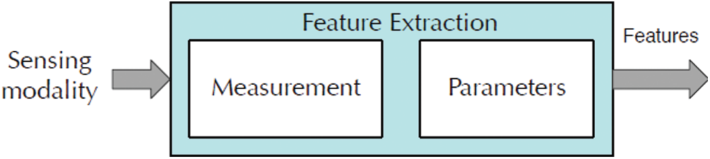
Figure 2: Process of the feature extraction

3.6.1 Improved Principal Component Analysis (IPCA)

. Principal Component Analysis (PCA) works as a tool to build predictive systems in investigative data analysis. Most often, the genetic distance and relatedness within the populations are visualized through PCA. PCA can be carried out through decomposition or eigenvalue data decomposition of correlation/covariance matrix, generally in post-normalization of initial data. Usually, there is a mean center in each attribute when normalizing it, which subtracts the value of each data from the measured mean of its variable; hence the corresponding empirical mean (i.e., average) becomes ‘zero’.

Consequently, it normalizes the variance of each variable as much as possible for assuming it ‘1’; see Z-scores. The component scores, also termed factor scores (the converted variable values associated with a specific data point), loadings (weight required to manipulate each original standardized variable for deriving the component score), and the PCA outcomes are considered conferred. If the standardization of component scores matches with unit variance, it indicates the existence of data variance in loadings and signifies that it is the magnitude of eigenvalues; whereas, the non-standardized component scores indicate that the data variance is accompanied by component scores only, and the loadings need to be unit-scaled (“normalized”). These weights are termed Eigenvectors, which are orthogonal rotation cosines of variables into principal components or back.

Generally, an internal data structure can be depicted by the functionality of this model, thereby the variance in the data in an optimal manner. In the context where the multivariate dataset is visualized as coordinates set in high-dimensional data space, PCA can offer lower-dimensional images to the user, during which the object is projected at its most informative perspective. This is possible only through a few standard components; thus, the dimensionality reduction is carried out in the transformed data. Nevertheless, if the outliers exist in the data set, PCA’s analysis result will be highly hampered. In such a scenario of huge data volume, it becomes a challenging task to separate the outliers. To overcome this issue, the Adaptive Gaussian kernel matrix is built.

3.6.2 Constructing the Adaptive Gaussian Kernel Matrix

In a distributed setting, assume s nodes set be V = {vi, 1 ≤ i ≤ s}, where everyone is capable of communicating central coordinator ‘v0’.

A local data matrix Pi ∈ Rni × d on each node ‘vi’ possesses ‘ni’ data points in ‘d’ dimension (ni > d). Subsequently, global data P∈Rn×d become local data matrix concatenation PT=[P1T,P2T,…,PsT] and n=∑i=1s⁡ni. The P’s ith row is denoted by pi. Consider centred data points with zero mean, i.e., ∑i=1spi=0 Uncentered data necessitates a rank-one modification in algorithms, whose computation and those in other steps dominate communication cost. Take on non-linear transformation ϕ(x) to M-dimensional new feature space from standard D-dimensional feature space; however, it demands extreme expense and inadequacy. Therefore, apply kernel methods for simplifying the computation.

Assume projected new features having zero mean, Eq. (9)

1N∑i=1N⁡ϕ(xi)=0(9)

The projected features covariance matrix is M × M, which can be projected as, Eq. (10)

C=1N∑i=1N⁡ϕ(xi)ϕ(xi)T(10)

Its eigenvectors and eigenvalues are as follows, Eq. (11)

Cvk=λkvk.(11)

Here, k = 1, 2,…, M. From expression Eqs. (10) and (11), have, Eq. (12)

1N∑i=1N⁡ϕ(xi){ϕ(xi)Tvk}=λkvk,(12)

The above expression can be rewritten as follows, Eq. (13)

vk=akiϕ(xi)(13)

Here, by substituting vk in Eq. (12) with Eq. (13), have, Eq. (14)

1N∑i=1N⁡ϕ(xi)ϕ(xi)T∑j=1N⁡akjϕ(xj)=λk∑i=1N⁡akiϕ(xi).(14)

The following equation expresses the kernel function, Eq. (15)

k(xi,xj)=ϕ(xi)Tϕ(xj),(15)

Then, multiply both sides of Eq. (16) by (xl)T, and get

1N∑i=1N⁡k(Xl,Xi)∑j=1N⁡akjk(Xi,Xj)=λk∑i=1N⁡akik(Xl,Xi)(16)

Here, the matrix notation is used as, Eq. (17)

K2ak=λkNKak(17)

In which, Eq. (18)

Ki,j=k(Xi,Xj)(18)

and ak denotes aki’s N-dimensional column vector, Eq. (19)

ak=[ak1ak2…akN]T(19)

ak might be estimated through Eq. (20)

Kak=λkNak,(20)

Then, the ensuing kernel principal components might be estimated as follows, Eq. (21)

yk(X)=ϕ(X)Tvk=∑i=1N⁡akik(X,Xi).(21)

The kernel approaches’ power is that it does not calculate ϕ(xi) explicitly. From training data set {xi}, kernel matrix is constructed directly, Eqs. (22) and (23)

k(x,y)=(xTy)d(22)

or k(x,y)=(xTy+c)d,(23)

In which c > 0 is a constant, and Gaussian kernel, Eq. (24)

k(x,y)=exp(−x−y2/2σ2)(24)

σ denotes an Adaptive Gaussian kernel parameter.

When k = 1, PCA becomes a special case, and the center is an r-dimensional subspace. This optimum r-dimensional subspace is spanned through top r right P singular vectors (principal components) that can be identified through Singular Value Decomposition (SVD).

3.7 Hybrid Learning Classifier Model (Hlcm)

The inputs of the IoT sensor network reached each neuron layer, during which the processes such as aggregation, pre-processing and feature extraction are carried out. To proceed further, healthcare data are predicted using Hybrid Learning Classifier Model (HLCM). Besides hybridising Deep Belief Neural Network (DBNN), SVM is carried out to predict healthcare data.

3.7.1 Deep Belief Neural Network (DBNN)

Being a feed-forward method, DBNN helps for connecting layers with every node in a multilayer perceptron. Since there are various parameters in the neural network, the output is generated with noisy information and error if the input signal is provided to the corresponding input network. Hence, for reducing the error rate, the partial derivatives of each variable are employed in this study. In feed-forward context, input to hidden layer from information layer is multiplied with specific weights. Consequently, every data source obtained by each shrouded node is summed up. Here, through the activation function, value is passed. Besides, quantities from the hidden layer for the yielding layer multiplied by different weights, and input obtained by yield is summed up. Again, the sum is passed through the activation function, and then the yield is generated. In a neural network, the target output is differentiated by the yield from the output layer.

By using the learning algorithm procedure, DBNN computation searches error function base in weight space. The combination of loads is considered an optimal solution for resolving the learning issue since it restricts the blunder capability. According to this procedure, the error function’s coherence and differentiability need to be ensured since the inclination of the learning algorithm needs to be estimated at each cycle.

In other words, such kind of enablement work needs to be utilized instead of progression capacity utilized in perceptions. Besides, the error function as to the output network layer needs to be computed. The network’s efficient learning process enhances the recognition process, and activation of function exists.

Meanwhile, the estimated output values are compared to the output of the pre-trained network. The comparison ensures accurate output, i.e., if both outputs are equal or indicate error propagation. In this process, the recognition rate can be improved by updating the values of weights and bias. In this study, the list of values, the selection of optimized weights is carried out with the help of SVM that is recognized as a global classification algorithm.

Besides, optimized extremum (minimum/maximum) values of weights can be predicted through this algorithm, and even the error value exists in the network. Subsequently, the current value is switched by the extremum selected points, and it is selected iteratively, concerning the Enhancement of recognition rate.

3.7.2 Support Vector Machine (SVM)

SVM is also called Maximum Margin Classifiers since it can perform the empirical classification error minimization and maximization of geometric margin concurrently. Moreover, SVM implicitly maps its inputs as high-dimensional feature spaces by employing kernel trick; hence it is recognized as an effective model for non-linear classification. The construction of the classifier is enabled by the kernel trick, regardless of clear indication about feature space. In SVM, the examples are represented as a point in space that is mapped. To differentiate the examples that belong to different classes, they are separated with possibly a considerable gap. Assume that a set of points is provided, which is from either of two classes, then a hyperplane accompanied by the most considerable possible points fraction belonging to the same class on the same plane will be identified by SVM. This separating hyperplane is termed as Optimal Separating Hyperplane that could increase distance in the middle of two parallel hyperplanes and the diminishing test dataset’s misclassifying examples risk. Labelled training data as data points with the form is specified in Eq. (25)

M={(x1,y1),(x2,y2),…,(xn,yn)}(25)

Here yn=1/−1 is a constant, which represents the class to which that point xnbelongs, in which the data sample’s count is signified by n.

A ‘real vector with p-dimension’ is denoted by each xn. At first, input vectors are mapped into a decision value by the SVM classifier, classified through a suitable threshold value. The hyperplane is divided as follows for viewing training data, Eq. (26)

Mapping:wT.x+b=0(26)

The ‘weight vector with p-dimension’ is signified by w, and ‘a scalar’ is denoted by b. The vector ‘w’ points are perpendicular for separating the hyperplane. Maximization of margin is enabled through the offset parameter b. These hyperplanes can be selected if t training data are linearly separable. Consequently, the distance between hyperplane will be tried to get maximized, as there are no points between them. At this point, the distance between the hyperplane as 2/|w| will be estimated. Minimization of |W|, needs to be ensured, Eq. (27)

w.xi−b≥1orw.xi−b≤−1(27)

3.7.3 Radial Basis Kernel Function

In higher-dimensional data, the RBF kernel function is efficient; hence, the SVM’s Radial Basis Function (RBF) kernel is deployed as Classifier. The kernel output relies on the Euclidean distance, of which one is the testing data point, and another one is the support-vector. At the centre of RBF, the support vector determines its area of impact across the data space. The following equation expresses RBF Kernel function, Eq. (28)

k(xi,xj)=exp⁡(−γ‖xi−xj‖2)γ>0(28)

In the above equation, a kernel parameter is denoted by k, defined as a training vector. Since RBF enables a support vector to influence more across a larger area, it is proven that a large area can efficiently support a more traditional decision boundary and a smoother decision surface. Besides, the application of optimal parameter on the training dataset eases the procurement of the classifier. Thus, efficient healthcare data classification can be performed through the developed hybrid learning classifier model where ‘k’ is a training vector and kernel parameter. And smooth decision surface is provided by a large value of highly regular decision boundary and smooth decision surface. Support vector can have a strong influence over a larger area by a RBF of large value. The training dataset is applied with the best parameter to obtain the classifier. Health care data are classified effectively using a designed hybrid learning classifier model.

4  Results and Discussion

In this segment, the proposed context-aware data fusion approaches are conferred, specifically for healthcare applications. In this work, the (Mobile HEALTH(MHEALTH) dataset is used for the suggested approach performance assessment.

Dataset Description

In the dataset of MHEALTH, the information such as body motion and vital signs recordings for ten volunteers are significantly involved, accompanied by different profile and numerous physical activities. For measuring the motion of different body parts (e.g., magnetic field orientation, acceleration, and rate of turn), the sensors are placed over the chest, left ankle, and right wrist of the subject. Besides, 2-lead ECG measurements are obtained by a sensor placed over the chest, through which primary heart monitor, various arrhythmias checking or monitoring exercise impacts on ECG are performed.

In order to evaluate different performance parameters, False Positive (FP), False Negative (FN), True Positive (TP) and True Negative (TN) values are estimated initially. The parameters, namely Accuracy, F-measure, Recall and Precision, are predominantly considered for measuring the performance.

Precision refers to the ratio between the number of appropriately identified positive instances and totally expected positive instances count, Eq. (29)

Precision=TP/TP+FP(29)

Recall or Sensitivity is defined as the ratio between the number of appropriately identified positive instances and total instances count, Eq. (30)

Recall=TP/TP+FN(30)

F-measure refers to the Recall and Precision’s weighted average. Such that, F-measure takes false positives and negatives, Eq. (31)

F1Score=2∗(Precision∗Recall)/(Precision+Recall)(31)

Based on the positives and negatives, the Accuracy is measured as expressed below, Eq. (32)

Accuracy=(FP+TP)/(TP+FP+TN+FN)(32)

Tab. 1 illustrates the performance comparison results of the proposed methodology. The table values show that the proposed hybrid model has high performance than the existing model.

In Fig. 3, the performance of the proposed and prevailing Context-aware data fusion methods is compared in terms of Precision rates for the healthcare data classification. From the figure, the graphs represent the efficiency of the proposed CDFT-HLCM method to provide optimal Precision rates, which is higher than the existing classification methods.

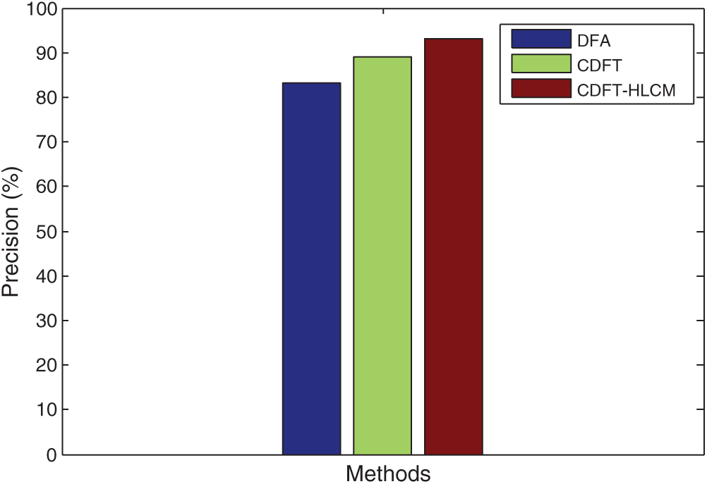
Figure 3: Analysis of precision context-aware data for classifying the healthcare data

Fig. 4 compares the Recall rates obtained by the proposed and prevailing Context-aware data fusion methods regarding healthcare data classification. The graphs represent that the proposed CDFT-HLCM method is proficient in procuring optimal Recall rates, which is superior to the existing classification.

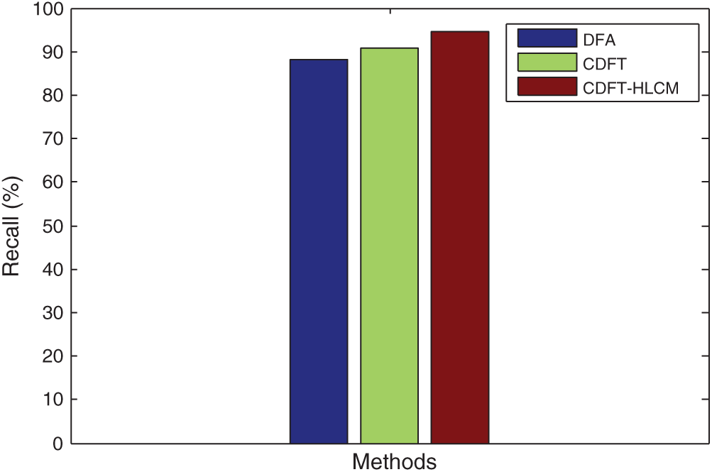
Figure 4: Analysis of recall context-aware data for classifying the healthcare data

Fig. 5 compares suggested and prevailing Context-aware data fusion methods’ F-measure values regarding healthcare data classification. It is substantiated that the suggested CDFT-HLCM method can obtain optimal F-measure values, which is higher than the existing classification methods.

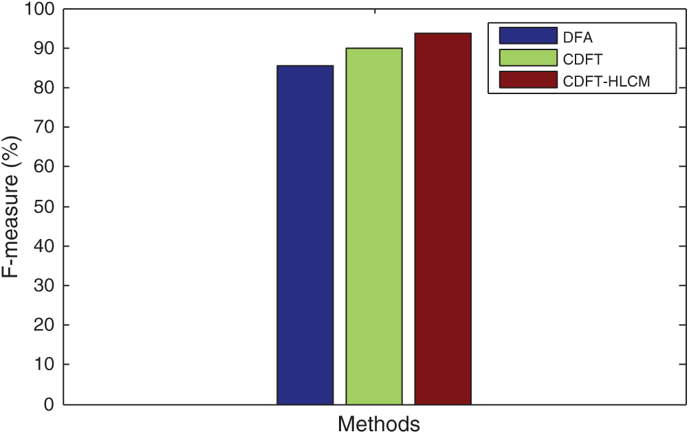
Figure 5: Analysis of F-measure context-aware data for classifying the healthcare data

In Fig. 6, the proposed and prevailing Context-aware data fusion methods are compared in terms of Accuracy rates for healthcare data classification. The graphs represent the efficiency of the proposed CDFT-HLCM method to provide better Accuracy rates, which is higher than the existing classification methods.

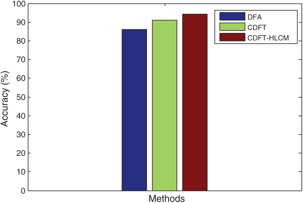
Figure 6: Analysis of accuracy context-aware data for classifying the healthcare data

5  Conclusion

This study proposes and assesses a Hybrid Learning Classifier Model (HLCM) based Context-aware Data Fusion technique for healthcare applications. Besides, for healthcare systems, data management phases, like pre-processing, feature extraction, data processing and storage and context-aware data fusion have been described in this research study. In addition, the data fusion process is carried out accurately with the help of a dual filtering technique that tends to label the unlabelled attributes in the accumulated data. Subsequently, feature extraction and dimension reduction take place through Improved Principal Component Analysis (IPCA). Then, the HLCM helps to learn this data, through which the efficiency of data fusion can be validated. At this point, hybridization of DBNN, SVM is accomplished with regards to healthcare data prediction. The proposed HLCM has 94.40% of accuracy than the other models. Empirical findings prove the efficiency of the proposed context-aware data fusion technique to outperform the static systems since the static systems utilize each available sensor statically. In the future, this research work can be further extended by focusing on the scrutiny of the proposed technique’s generalization capability, for which the training and test data from various scenarios can be taken. Besides, the security enhancement of the predicted healthcare data can be considered.

Funding Statement: The authors received no specific funding for this study.

Conflicts of Interest: The authors declare that they have no conflicts of interest to report regarding the present study.

This work is licensed under a Creative Commons Attribution 4.0 International License, which permits unrestricted use, distribution, and reproduction in any medium, provided the original work is properly cited.