DOI:10.32604/cmc.2022.019369
| Computers, Materials & Continua DOI:10.32604/cmc.2022.019369 | |
| Article |
Comparison of Missing Data Imputation Methods in Time Series Forecasting
1Division of Software Convergence, Hanshin University, Gyeonggi, 18101, Korea
2Contents Convergence Software Research Institute, Kyonggi University, Gyeonggi, 16227, Korea
3Division of AI Computer Science and Engineering, Kyonggi University, Gyeonggi, 16227, Korea
*Corresponding Author: Kwanghoon Pio Kim. Email: kwang@kyonggi.ac.kr
Received: 11 April 2021; Accepted: 23 May 2021
Abstract: Time series forecasting has become an important aspect of data analysis and has many real-world applications. However, undesirable missing values are often encountered, which may adversely affect many forecasting tasks. In this study, we evaluate and compare the effects of imputation methods for estimating missing values in a time series. Our approach does not include a simulation to generate pseudo-missing data, but instead perform imputation on actual missing data and measure the performance of the forecasting model created therefrom. In an experiment, therefore, several time series forecasting models are trained using different training datasets prepared using each imputation method. Subsequently, the performance of the imputation methods is evaluated by comparing the accuracy of the forecasting models. The results obtained from a total of four experimental cases show that the
Keywords: Missing data; imputation method; time series forecasting; LSTM
The recent emergence of cutting-edge computing technology such as the internet of things (IoT) and big data, has resulted in a new era in which large-scale data can be generated, collected, and exploited. By combining unstructured data created from various data-generating sources with well-structured data that are primarily used for data analysis, not only the data volume but also information and knowledge that were previously difficult to obtain can now be acquired more easily.
Among the wide array of data classes, time series, which is a sequence of data arranged in chronological order (i.e., a typical type in data analysis), has many real-world applications in various domains, such as energy [1,2], climate [3], economics [4], business [5] and healthcare [6]. The use of a significant amount of time series data that can be obtained via sensors and computing devices that have evolved in recent years might enhance analysis and forecasting abilities for solving real-life problems. Nevertheless, many data analysis studies have empirically confirmed that numerous missing values often coexist within such rich data. These missing values are considered as major obstacles in data analysis because they distort the statistical properties of the data and reduce availability. In particular, in time series modeling where it is critical to capture correlations with past data, missing values may significantly impair the performance of time series analysis and forecasting.
To address the missing data problem, which is inevitable in real-life data analysis, various imputation techniques for reconstructing missing values have been primarily investigated in the field of statistics [7–10]. In this regard, this paper presents experimental results for evaluating the effect of imputation on time series forecasting performance by applying well-adopted imputation methods to multivariate time series datasets. An intuitive approach to confirm the effect of imputation is to estimate the values of the deliberately introduced missing data and quantitatively measure their similarity to the ground truths of the missing parts [11]. However, this approach presents two limitations. First, artificial missing values are part of the results of a simulation, which cannot consider missingness occurring in the real world that is affected by numerous factors and their dependence. Second, when analyzing real data, incomplete data with a high missing rate are likely to be encountered. Hence, the ground truths of missing data cannot be obtained, and a significant portion of the data cannot be evaluated.
The experiment performed in this study was designed to avoid the shortcomings mentioned below. First, incomplete data are filled with estimated values by imputing the actual missing values instead of introducing artificial missing parts. Next, individual forecasting models were trained from different datasets recovered by each imputation method. Subsequently, the performances of the forecasting models were measured on a common test set, and the effectiveness of each imputation method was evaluated and compared with those of other methods. We exploited six imputation methods provided as a Python library that is easily accessible and used by non-technical people. In addition, four datasets of multivariate time series including actual missing data were used in the experiments.
The remainder of this paper is organized as follows. In Section 2, the basic missing types are defined, and related studies involving the imputation of missing values within a time series are summarized. Section 3 provides definitions of missing value imputation and the main related techniques. Section 4 presents the experimental results for the evaluation and comparison of the imputation methods. Section 5 provides the conclusions and future research directions.
Missing values are often encountered in many real-world applications. For example, when obtaining data from a questionnaire, many respondents are likely to intentionally omit a response to a question that is difficult to answer. As another example, when collecting data measured by machines or computer systems, various types of missing values can occur owing to mechanical defects or system malfunctions. Because missing values have undesirable effects on data availability and quality, handling such missing values should be considered in data analysis. To devise an optimal strategy for deciding how to handle missing values, the underlying reasons contributing to the occurrence of missing values must be understood. The primary types of missing values identified in previous studies related to the field of statistics are as follows:
• Missing completely at random (MCAR): This indicates that the missingness of data is independent of both observed and unobserved variables. The MCAR assumption is ideal in that unbiased estimates can be obtained regardless of missing values; however it is impractical in many cases of real-world data [7].
• Missing at random (MAR): Missingness is related to observed but not unobserved variables. A dataset that holds the MAR assumption may or may not result in a biased estimate.
• Missing not at random (MNAR): Missingness is related to unobserved variables, i.e., missing values originate from events or unknown factors that are not measured. Similar to MAR data, a dataset that holds the MNAR assumption may or may not result in a biased estimate.
Whereas analysis on a dataset with MCAR outputs unbiased results, a dataset with MAR or MNAR, which comprise the majority of real-world data, requires the appropriate treatment to alleviate estimate biases. This can be solved using several methods, however, in this study, we focused on imputation methods that replace missing values in an automated manner.
In terms of time series data, missing values might be the primary cause of distortion in the statistical properties of the data. In particular, for time series that are highly correlated with themselves in the past, the improper handling of missing values may result in inaccurate results in analysis tasks (e.g., time series forecasting). For example, if a simple solution for handling missing values, such as case deletion, is applied to time series data regardless of the data characteristics, it is highly likely to fail in the modeling of temporal dependencies, resulting in degraded model predictive power. However, the appropriate use of the imputation method, which recovers missing values through numerical or algorithmic approaches, yields more reliable time series analysis results.
Various univariate imputation methods [12–14] that reconstruct the missing values of a single variable based on time dependence can be used as the simplest form of imputation. In [12], univariate imputation methods such as mean substitution, last observation carried forward (LOCF), linear interpolation, and seasonal Kalman filter [15] were compared in terms of imputation accuracy. In an experiment, the missing values in the dataset were randomly generated; subsequently, the imputation accuracy of each method was measured based on the differences between the imputed and actual values. The results show that the Kalman filter method is the most effective for univariate imputation. In addition, [13] attempted univariate imputation using statistical time series forecasting models such as autoregressive integrated moving average (ARIMA) and its variant, SARIMA for seasonality modeling. The authors of [14] proposed a univariate imputation method based on dynamic time warping (DTW). First, DTW is performed to identify a time series that includes a subsequence that is the most similar to a subsequence before the missing part. Then, the missing part is replaced by the next subsequence of the most similar one. However, since many time series are multivariate and contain covariates between variables, the range in which univariate imputation methods can be effectively applied is limited.
As correlations between variables generally exist in real-world data, multivariate imputation is likely to be more effective than univariate imputation. In this regard, the k-nearest neighbors (k-NN [8]), expectation-maximization (EM [16]), local least squares (LLS [17]), and probabilistic principal component analysis (PPCA [10]) have been widely applied in multivariate imputation. As a comparative study, [18] performed a benchmark analysis on traffic data using various multivariate imputation methods. The results showed that the PPCA achieved the best performance among the methods. Meanwhile, multiple imputation by chained equation (MICE [19]), which selects a single value among several imputed values, is another technique for multivariate imputation.
With the advent of big data, imputation techniques based on deep neural networks {[20–22,11]} that are capable of capturing nonlinear temporal dynamics have garnered significant attention. Recurrent neural network (RNN) is a representative deep learning model designed for sequential data and has been widely used for natural language processing (NLP) and time series forecasting. Because RNNs can model temporal dependencies, those variants combined with the encoder-decoder framework [20,22] for many-to-many predictions or the bidirectional feed forwarding process [21] were devised and demonstrated to be competitive in reconstructing missing values. In addition, there have been attempts to perform imputation by combining machine and deep learning models with optimization techniques such as the Monte Carlo Markov chain [23] and collaborative filtering [24]. These state-of-the-art methods are excellent at generating accurate imputation results when large-scale data are available. However, many of these are not generally used by non-technical people because they are seldom distributed in user-friendly packages or do not provide reproducibility.
In this study, we analyzed the effect of the imputation process on the time series forecasting performance using several imputation techniques that are suitable for time series data and easily accessible. In the benchmark studies [12,18] described above, missing values are generated artificially first, and then the performance of imputation methods are compared by measuring prediction losses, which indicate the difference between the imputation results and the ground truth values. By contrast, our benchmark does not impose missing values into the datasets; instead, it exploits datasets that originally contain missing data. Because the actual values for the missing parts are unknown, the imputation performance is evaluated by measuring the accuracy of the forecasting models generated by each imputation method.
3 Imputation Methods for Time Series
This section introduces the concept of missing data imputation in the time series and the imputation methods used in the experiments. We assume a multivariate time series
The imputation of a missing feature is defined as
For an incomplete time series, the simplest method to handle missing features is to exclude observations that contain a missing feature (e.g., pairwise and listwise deletion). However, these approaches may degrade the availability of data and yield biased estimates [25]. Therefore, methods that involve uniformly replacing missing features with a specific value are used more frequently (e.g., mean substitution). For all missing features
If the data provides missing parts of non-trivial size, then the missing values must be estimated using an elaborate procedure rather than the simple approaches mentioned above. In general, two types of imputation scenarios exist for replacing missing values with plausible values: univariate and multivariate imputation. The most intuitive technique for univariate imputation is the LOCF method, which carries forward the last observation before the missing data. Recalling the example above, the missing feature of
For a multivariate time series, the correlations between variables must be modeled. The EM algorithm [16] is a model-based imputation method that is frequently applied in multivariate imputation, and it repeatedly imputes missing values based on maximum likelihood estimation. The k-NN algorithm is another effective solution for the multivariate imputation method. For an instance in which missing occurs, the
In this study, the effect of missing value imputation in the time series forecasting problem was evaluated experimentally according to the procedure shown in Fig. 1. The first step is to obtain a refined dataset through data preprocessing steps, such as data cleansing, transformation, and reduction. Next, imputation methods are used to fill in the missing values in the dataset. For this procedure, we exploited six imputation methods: mean substitution, LOCF, NOCB, EM, {k-NN}, and MICE. Subsequently, the individual forecasting models were trained with each imputed dataset. Finally, the performance of the forecasting models was evaluated and compared using loss functions.
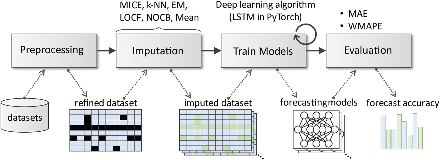
Figure 1: Overall experimental procedure
We used four datasets of multivariate time series as experimental data to train and validate the time series forecasting models. The datasets were obtained from [26,27] and contained actual missing values of different patterns. A summary of the datasets used in the experiments is provided in Tab. 1.
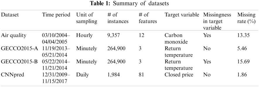
The dataset (Air Quality) was originally provided to predict benzene concentrations to monitor urban pollution [28]. This dataset contains 9,357 instances of hourly averaged responses from an array of five metal oxide chemical sensors embedded in an air quality chemical multisensory device. The device was placed in a significantly polluted area at the road level, within a city in Italy. For the experiment in this study, we excluded some features with abnormally high missing rates from the original dataset, and the reorganized dataset had a missing rate of 13.35%. The hourly average concentrations of carbon monoxide (CO) were used as target variables.
The dataset was originally provided by the Genetic and Evolutionary Computation Conference (GECCO) Industrial Challenge 2015 [27] to recover missing data in a heating system. Observations from the dataset were measured every minute via a closed-loop heating system and comprised four time series: the system temperature setpoint, system supply temperature, system power, and return temperature (target variable). The original dataset comprised 604,800 instances from November 19, 2013 to December 1, 2015. For this experiment, we prepared two sub-datasets with different patterns of missing data from the original dataset. The first sub-dataset (GECCO2015-A) consisted of a total of 264,900 observations between November 2013 and May 2014, with a missing ratio of 5.46% and no missing target variable. The second sub-dataset (GECCO2015-B) had the same data length as GECCO2015-A and included observations from May 2014 to November 2014. The missing rate was 15.69%, which was relatively higher than that of GECCO2105-A; in particular, it was discovered that the target variable contained missing values.
The CNNpred dataset was first published in a study for predicting stock prices using convolutional neural networks [29]. It contains several daily features related to stock market indexes in the U.S., such as the S&P 500, NASDAQ Composite, and Dow Jones Industrial Average from 2010 to 2017. Specifically, CNNpred includes features from various categories of technical indicators, future contracts, prices of commodities, important market indices, prices of major companies, and treasury bill rates. In contrast to the other three datasets, CNNpred is a small-sized dataset with a feature space of relatively high dimensionality (1,984 instances and 81-dimensional features); additionally, it had the lowest missing rate (1.86%) and a complete non-missing target variable.
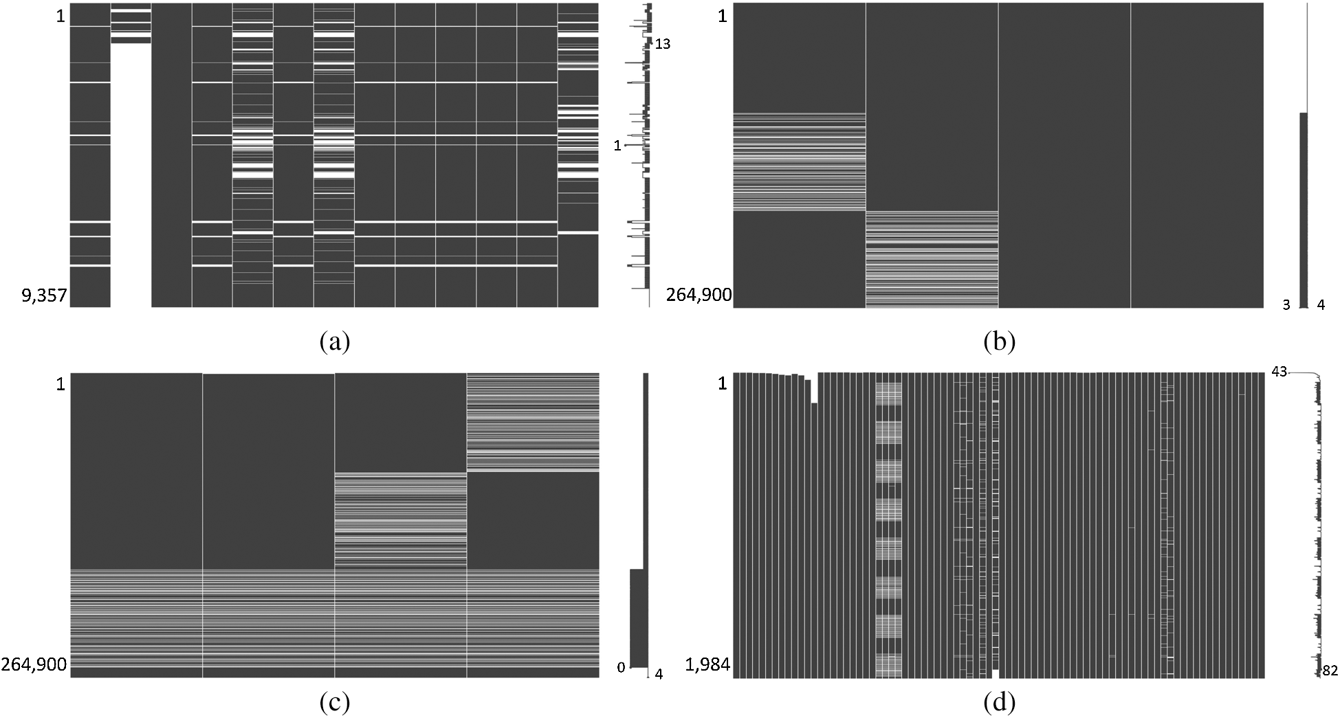
Figure 2: Missing patterns of datasets (a) Air quality (b) GECCO2015-A (c) GECCO2015-B (d) CNNperd
Fig. 2 shows the different missing patterns for each dataset. Each column corresponds to an individual feature, and the rightmost column represents the target variable. The missing parts are represented as blank spaces to indicate the number of missing values in each feature. The sparklines on the right side of each subfigure represent the number of observed values for each data instance. For the case shown in Fig. 2a, 1 on the sparkline represents that only one value available within that instance, whereas the remaining values are missing. By contrast, 13 indicates that all the values, including the target variable, are observations without missingness.
Depending on whether the target variable contains missing values, we applied different imputation processing to each dataset. For the datasets shown in Figs. 2a and 2c, instances exist where the target variable is missing. In cases of instances in the training set, all missing values, including the target variable, were estimated by imputation, as shown in Fig. 3. However, if an instance is within the test set, then the prediction loss cannot be measured without its ground truth; therefore, that instance is excluded from the dataset (case deletion). Conversely, the datasets, shown in Figs. 2b and 2d, contain complete target variables. Therefore, all missing values are imputed regardless of the set to which the instance belongs.
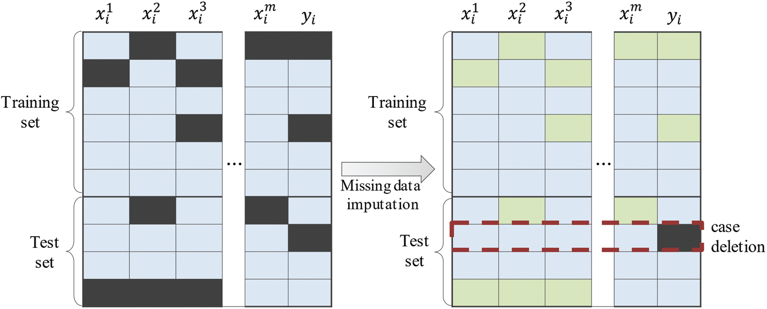
Figure 3: Two different methods of handling missing values: imputation and case deletion
4.2 Long Short-Term Memory-Based Forecasting Model
Long Short-Term Memory (LSTM) is a deep learning model for learning sequence data that can be applied widely, such as in natural language processing [4], human action recognition [30], and time series forecasting [2]. In LSTM neural networks, three gating mechanisms are implemented, thereby providing advantages to gradient vanishing/exploding problems, which are significant disadvantages of machine learning models based on artificial neural networks. As shown in Fig. 4, an LSTM cell is a building block of LSTM networks and takes three inputs at time step
An input gate decides the new information to be stored in
Subsequently, the older cell state
An output gate produces the final output of an LSTM cell. First, through a sigmoid activation function,
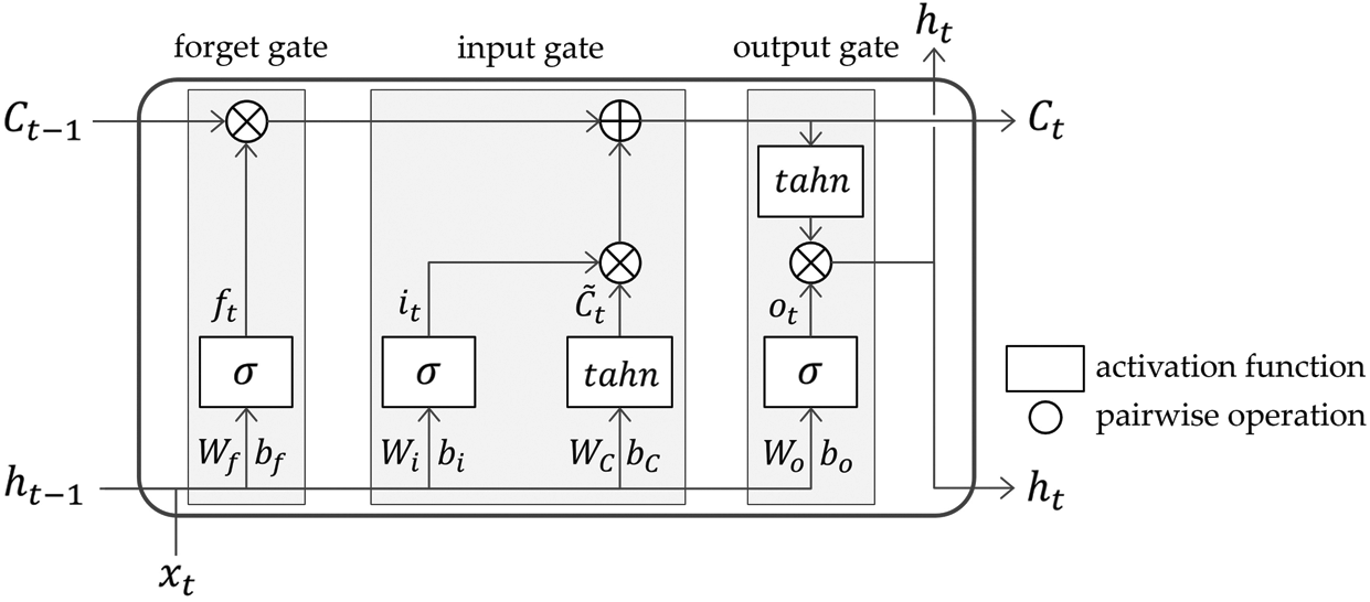
Figure 4: Structure of LSTM cell
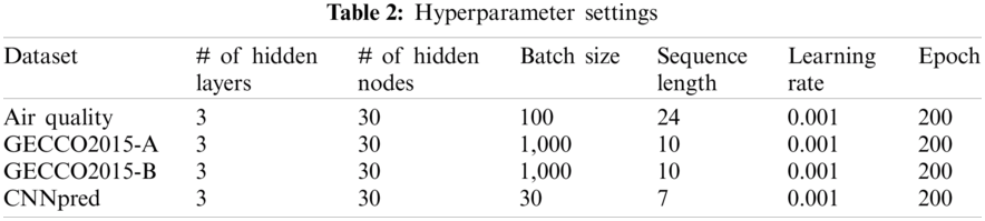
Based on LSTM neural networks, we constructed time series forecasting models that use different training sets generated by each imputation method. Tab. 2 represents the hyperparameter settings for the training forecasting models for each dataset. Through preliminary experiments, we confirmed that the number of hidden layers and nodes slightly affected the model performance. Therefore, we set these two hyperparameters to 3 and 30, separately for all the datasets. In addition, the batch size and sequence length were assigned with different parameter values based on the dataset size.
To evaluate the performance of the forecasting models, two loss functions, i.e., the mean absolute error (MAE) and weighted mean absolute percentage error (WMAPE), were used as scale-independent metrics. They are defined as follows:
where
Tab. 3 shows a comparison of the results obtained from the performance measurements of the forecasting models for each imputation method. For each dataset, the best and worst cases are shown in blue and red, respectively. Compared with other methods, k-NN demonstrated the best results for three datasets (Air Quality, GECCO2015-A, and CNNpred). In the case of CNNpred with the lowest missing rate (1.86%), the results indicate that k-NN widened the performance gap compared with the other methods. For instance, k-NN outputs a WMAPE value of
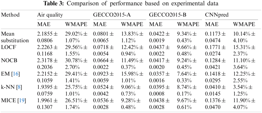
In summary, we confirmed that k-NN outperformed the other imputation methods in three among four datasets. It ranked second only in GECCO2015-B, whose target variable contained many missing parts. If missing values are few and the target variable is complete in a specified dataset, then k-NN would be an attractive imputation technique for achieving stable time series forecasting performance. In addition, we conclude from the results that multivariate imputation methods are generally superior to univariate imputation methods because most time series in real-life are multivariate and include relationships between variables.
In terms of threats to validity, we investigated only a small set of conventional imputation methods, not including many state-of-the-art imputation techniques (e.g., deep-learning-based models). In addition, because the simulation approach based on major assumptions (MCAR, MAR, and MNAR) that relate to the occurrence type of missing values was not included in the experiment, it is difficult to argue that the experimental results of this study elicit a general conclusion on the effect of missing data imputation. Therefore, to derive more significant benchmark results, a wider variety of imputation techniques and missing scenarios should be investigated in the future.
Missing values are a significant obstacle in data analysis. In time series forecasting, in particular, handling missing values in massive time series data is challenging. In this study, we evaluated the effects of imputation methods for replacing missing values with estimated values. We attempted to indirectly validate the imputation methods based on the performances of time series forecasting models, instead of using an approach that generates virtual missing data by simulation. The experimental results show that k-NN yielded the best model performance among the selected imputation methods.
Owing to the limitations of the results, we plan to conduct a more sophisticated benchmark study that can be extended to more imputation approaches, including machine learning techniques, while considering several missing-data scenarios. In addition, by conducting an experiment to investigate the efficacy of the imputation process in reconstructing missing values introduced by simulation, we hope to investigate the imputation effect more comprehensively.
Acknowledgement: The authors would like to thank the support of Contents Convergence Software Research Institute and the support of National Research Foundation of Korea.
Funding Statement: This research was supported by Basic Science Research Program through the National Research Foundation of Korea (NRF) funded by the Ministry of Education (Grant Number 2020R1A6A1A03040583).
Conflicts of Interest: The authors declare that they have no conflicts of interest to report regarding the present study.
1. F. Wahid, L. H. Ismail, R. Ghazali and M. Aamir, “An efficient artificial intelligence hybrid approach for energy management in intelligent buildings,” KSII Transactions on Internet and Information Systems, vol. 13, no. 12, pp. 5904–5927, 2019. [Google Scholar]
2. B. Lee, H. Lee and H. Ahn, “Improving load forecasting of electric vehicle charging stations through missing data imputation,” Energies, vol. 13, no. 18, pp. 4893, 2020. [Google Scholar]
3. W. Yu, H. Zhang, T. Chen, J. Liu and Y. Shen, “The analysis of climate change in Haiyan county,” KSII Transactions on Internet and Information Systems, vol. 14, no. 10, pp. 3941–3954, 2020. [Google Scholar]
4. J. Zhang, J. Zhang, S. Ma, J. Yang and G. Gui, “Chatbot design method using hybrid word vector expression model based on real telemarketing data,” KSII Transactions on Internet and Information Systems, vol. 14, no. 4, pp. 1400–1418, 2020. [Google Scholar]
5. C. G. Park and H. Ahn, “Temporal outlier detection and correlation analysis of business process executions,” IEICE Transactions on Information and Systems, vol. 102, 7, no. 7, pp. 1412–1416, 2019. [Google Scholar]
6. I. Y. Ahn, N.-M. Sung, J.-H. Lim, J. Seo and I. D. Yun, “Development of an oneM2M-compliant IoT platform for wearable data,” KSII Transactions on Internet and Information Systems, vol. 13, no. 1, pp. 1–15, 2019. [Google Scholar]
7. D. B. Rubin, “Inference and missing data,” Biometrika, vol. 63, no. 3, pp. 581–592, 1976. [Google Scholar]
8. J. K. Dixon, “Pattern recognition with partly missing data,” IEEE Transactions on Systems, Man, and Cybernetics, vol. 9, no. 10, pp. 617–621, 1979. [Google Scholar]
9. A. P. Dempster, N. M. Laird and D. B. Rubin, “Maximum likelihood from incomplete data via the EM algorithm,” Journal of the Royal Statistical Society: Series B (Methodological), vol. 39, no. 1, pp. 1–22, 1977. [Google Scholar]
10. M. E. Tipping and C. M. Bishop, “Mixtures of probabilistic principal component analyzers,” Neural Computation, vol. 11, no. 2, pp. 443–482, 1999. [Google Scholar]
11. Y. Luo, X. Cai, Y. Zhang, J. Xu and X. Yuan, “Multivariate time series imputation with generative adversarial networks,” in Proc. NIPS, Montreal, Québec, Canada, pp. 1596–1607, 2018. [Google Scholar]
12. S. Moritz, A. Sardá, T. Bartz-Beielstein, M. Zaefferer and J. Stork, “Comparison of different methods for univariate time series imputation in R,” arXiv preprint arXiv: 1510.03924, 2015. [Google Scholar]
13. W. O. Yodah, J. M. Kihoro, K. H. O. Athiany and H. W. Kibunja, “Imputation of incomplete non-stationary seasonal time series data,” Mathematical Theory and Modeling, vol. 3, no. 12, pp. 142–154, 2013. [Google Scholar]
14. T.-T.-H. Phan, É. P. Caillault, A. Lefebvre and A. Bigand, “Dynamic time warping-based imputation for univariate time series data,” Pattern Recognition Letters, vol. 139, pp. 139–147, 2020. [Google Scholar]
15. A. Zeileis and G. Grothendieck, “Zoo: S3 infrastructure for regular and irregular time series,” Journal of Statistical Software, vol. 14, no. 6, pp. 1–27, 2005. [Google Scholar]
16. J. L. Schafer, Analysis of Incomplete Multivariate Data. New York, NY, USA: Chapman and Hall/CRC, 1997. [Google Scholar]
17. H. Kim, G. H. Golub and H. Park, “Missing value estimation for DNA microarray gene expression data: Local least squares imputation,” Bioinformatics, vol. 21, no. 2, pp. 187–198, 2005. [Google Scholar]
18. Y. Li, Z. Li and L. Li, “Missing traffic data: Comparison of imputation methods,” IET Intelligent Transport Systems, vol. 8, no. 1, pp. 51–57, 2014. [Google Scholar]
19. S. van Buuren, “Multiple imputation of missing blood pressure covariates in survival analysis,” Statistics in Medicine, vol. 18, no. 6, pp. 681–694, 1999. [Google Scholar]
20. Y. G. Cinar, H. Mirisaee, P. Goswami, E. Gaussier and A. Aït-Bachir, “Period-aware content attention RNNs for times series forecasting with missing values,” Neurocomputing, vol. 312, no. 3, pp. 177–186, 2018. [Google Scholar]
21. W. Cao, D. Wang, J. Li, H. Zhou, Y. Li et al., “BRITS: Bidirectional recurrent imputation for time series,” in Proc. NIPS, Montreal, Québec, Canada, pp. 6774–6784, 2018. [Google Scholar]
22. V. Fortuin, D. Baranchuk, G. Rätsch and S. Mandt, “GP-VAE: Deep probabilistic multivariate time series imputation,” in Proc. AISTATS, Palermo, Sicily, Italy, pp. 1651–1661, 2020. [Google Scholar]
23. C. Yozgatligil, S. Aslan, C. Iyigun and I. Batmaz, “Comparison of missing value imputation methods in time series: The case of Turkish meteorological data,” Theoretical and Applied Climatology, vol. 112, no. 1–2, pp. 143–167, 2013. [Google Scholar]
24. L. Li, J. Zhang, Y. Wang and B. Ran, “Missing value imputation for traffic-related time series data based on a multi-view learning method,” IEEE Transactions on Intelligent Transportation Systems, vol. 20, no. 8, pp. 2933–2943, 2018. [Google Scholar]
25. A. C. Acock, “Working with missing values,” Journal of Marriage and Family, vol. 67, no. 4, pp. 1012–1028, 2005. [Google Scholar]
26. A. Asuncion and D. Newman, “UCI machine learning repository,” 2007. [Online]. Available: https://archive.ics.uci.edu/ml/index.php. [Google Scholar]
27. SPOTSeven Lab, “GECCO (genetic and evolutionary computation conference) industrial challenge 2015,” 2015. [Online]. Available: https://www.spotseven.de/gecco/gecco-challenge/gecco-challenge-2015/. [Google Scholar]
28. S. De Vito, E. Massera, M. Piga, L. Martinotto and G. Di Francia, “On field calibration of an electronic nose for benzene estimation in an urban pollution monitoring scenario,” Sensors and Actuators B: Chemical, vol. 129, no. 2, pp. 750–757, 2008. [Google Scholar]
29. E. Hoseinzade and S. Haratizadeh, “CNNpred: CNN-based stock market prediction using a diverse set of variables,” Expert Systems with Applications, vol. 129, no. 3, pp. 273–285, 2019. [Google Scholar]
30. J.-C. Kim and K. Chung, “Prediction model of user physical activity using data characteristics-based long short-term memory recurrent neural networks,” KSII Transactions on Internet and Information Systems, vol. 13, no. 4, pp. 2060–2077, 2019. [Google Scholar]
 | This work is licensed under a Creative Commons Attribution 4.0 International License, which permits unrestricted use, distribution, and reproduction in any medium, provided the original work is properly cited. |