[BACK]
Computers, Materials & Continua
DOI:10.32604/cmc.2022.019345 |  |
| Article | |
Soft ζ-Rough Set and Its Applications in Decision Making of Coronavirus
M. A. El Safty1,*, Samirah Al Zahrani1, M. K. El-Bably2 and M. El Sayed3
1Department of Mathematics and Statistics, College of Science, Taif University, Taif, 21944, Saudi Arabia
2Department of Mathematics, Faculty of Science, Tanta University, Tanta, Egypt
3Department of Mathematics, College of Science and Arts, Najran University, Najran, 66445, Saudi Arabia
*Corresponding Author: M. A. El Safty. Email: m.elsafty@tu.edu.sa
Received: 9 April 2021; Accepted: 10 May 2021
Abstract: In this paper, we present a proposed method for generating a soft rough approximation as a modification and generalization of Zhaowen et al. approach. Comparisons were obtained between our approach and the previous study and also. Eventually, an application on Coronavirus (COVID-19) has been presented, illustrated using our proposed concept, and some influencing results for symptoms of Coronavirus patients have been deduced. Moreover, following these concepts, we construct an algorithm and apply it to a decision-making problem to demonstrate the applicability of our proposed approach. Finally, a proposed approach that competes with others has been obtained, as well as realistic results for patients with Coronavirus. Moreover, we used MATLAB programming to obtain the results; these results are consistent with those of the World Health Organization and an accurate proposal competing with the method of Zhaowen et al. has been studied. Therefore, it is recommended that our proposed concept be used in future decision making.
Keywords: Soft set; soft rough set; soft ζ rough set; COVID-19; intelligence discovery; decision making
1 Introduction
In 1999 Molodtsov [1] have introduced the soft set notion and progressing basics of this theory as a new diverse for modeling roughness and uncertainties. Diverse fields of applications of his approach were used in solving many practical problems in economics, engineering, social science, medical science… etc. Researchers have implementing various kinds of soft, rough and fuzzy sets (see [1–15]).
Often, the right decision making for many real-life issues is very difficult in our daily lives, which is highly essential for choosing the best solution to our discussions. Therefore, we have to consider various features in order to produce the highest practical solution to these problems. For this cause, we use the chosen mathematical instrument in the current article, namely soft rough set theory, in decision making. Decision making application was applied by Maji et al. [10,11]. Using soft set approach and accordingly they expand this approach to fuzzy soft set theory in [13]. Soft rough model was defined by [15].
Coronavirus emerged in 2019, in Wuhan, China. This virus is a new strain that has not been previously identified in humans. It was believed that Coronaviruses spread from dirty, dry surfaces, like automatic mucous membrane pollination in the nose, eyes, or mouth, reinforcing the importance of a clear understanding of the persistence of coronaviruses on inanimate surfaces [16]. Therefore, two factors which are in contact with infected surfaces and encounters with infected viruses, affect the transmission. As a result, many scientific papers have been published and many researchers have studied this virus, such as ([16–22]).
As a generalization to Pawlak’s rough models [23]. Based on this structure, they defined soft rough approximations, soft rough sets and some related concepts, such as ([23–27]).
The main objective of our belief is to have a certain influence on the continuous approximation of such basic mathematical principles and to provide a modern method for computational mathematics of real-life problems. In fact, it considers latest generalized soft, rough approximations, called soft ζ-rough approximations, are defined as a generalization to Zhaowen et al. [15] approximations and their properties are studied. We will prove that our approaches are more accurate and general from Zhaowen et al. approaches. The importance of the current approximations is not only that it is reducing or deleting the boundary regions, but also, it’s satisfying all properties of Pawlak’s rough sets without any restrictions. Comparisons between our method and the method of Zhaowen et al. are obtained.
Several examples are provided to illustrate the links between topologies and relationships of the soft set. Finally, we are added three applications. in making decisions regarding our strategy. One of them represents a beginning point for apply soft rough approach to solve the problem of Coronavirus contagion. At the end of the paper, we give two an algorithm which can be used to have a decision making for information system in terms of soft ζ-rough approximations.
The main programming for this paper is as follows:
Step 1: Input the set Ŵ and the set of features represent the data as an information table, rows of which are labeled by features A, columns by objects and entries of the table are features values.
Step 2: Compute the rough neighborhood from the information table.
Step 3: Compute the soft ζ-upper approximation, ζ-lower approximation and ζ-boundary for the decision set M⊆Ŵ.
Step 4: Remove a feature a1 from the condition’s features (A) and then find the rough neighborhood A-{a1}.
Step 5: Comparing ζ-boundary for the decision set M⊆Ŵ on A-{ai} with Step 3.
Step 6: Repeat Steps 4 and 5 for all attributes in A.
Step 7: Those attributes in A for which BNDA-{ai}ε(M)≠BNDAε(M) forms the Core (Ŵ).
Finally, we explain the importance of the proposed method in the medical sciences for application in decision-making problems. In fact, a medical application has been introduced in the decision-making process of COVID-19 Medical Diagnostic Information System with the algorithm. This application may help the world to reduce the spread of Coronavirus.
The paper is structured as follows: The basic concepts of the rough set and soft set were explored in section two and three. The implementation of COVID-19 for each subclass of attributes in the information systems and comparative analysis was presented in section four and five. Section six concludes and highlights future scope.
2 Preliminaries
In this section, we give some basic definitions and results that used in sequel are mentioned.
2.1 Pawlak Rough Set Theory
In 1982, Pawlak [23] introduced the theory of rough set as a new mathematical methodology or easy tools in order to deal with the vagueness in knowledge-based systems, information systems and data dissection. This theory has many applications in many fields that are used to process control, economics, such as medical diagnosis, chemistry, psychology, finance, marketing, biochemistry, environmental science, intelligent agents, image analysis, biology, conflict analysis, telecommunication, and other fields (See: [23–27], and the bibliography in these papers).
Definition 2.1 [23] Assuming that Ŵ be a set, and ℜ be an equivalence relation on Ŵ, we use Ŵ\ℜ the a collections of all equivalence classes of ℜ and [x]ℜ. It is indicated an equivalence class in ℜ containing an element x∈Ŵ. Then, the pair (Ŵ,ℜ) it’s called an approximation space and for every M⊆Ŵ, we can define the lower and upper approximation of M by ℜ(M)={x∈Ŵ:[x]ℜ⊆M} and ℜ¯(M)={x∈Ŵ:[x]ℜ∩M≠ϕ}, respectively.
According to Pawlak’s definition, M it’s called a rough set if R(M)≠ℜ¯(M).
Proposition 2.1 [23] Let ϕ be the empty set and Mc be the complement of M⊆Ŵ. Pawlak’s rough sets have the next characteristic:
L1 -ℜ(M)⊆MU1 M⊆ℜ-(M)L2 -ℜ(ϕ)=ϕU2 ℜ-(ϕ)=ϕL3 -ℜ(Ŵ)=ŴU3 ℜ-(Ŵ)=ŴL4 -ℜ(M∩N)=-ℜ(M)∩-ℜ(N)U4 ℜ-(M∪N)=ℜ-(M)∪ℜ-(N)L5 If M⊆N then -ℜ(M)⊆-ℜ(N)U5 If M⊆N the ℜ-(M)⊆ℜ-(N)L6 -ℜ(M)∪-ℜ(N)⊆-ℜ(M∪N)U6 ℜ-(M∩N)⊆ℜ-(M)∩ℜ-(N)L7 -ℜ(Mc)=(ℜ-(M))CU7 ℜ-(Mc)=(-ℜ(M))CL8 -ℜ(-ℜ(M))=-ℜ(M)U8 ℜ-(ℜ-(M))=ℜ-(M)L9 If M∈Ŵ/ℜ then -ℜ(M)=MU9 If M∈Ŵ/ℜ then ℜ-(M)=M 2.2 Soft Set Theory and Soft Rough Set
Let us recall now the soft set notion, which is a newly-emerging mathematical approach to vagueness. Let Ŵ be an initial universe of objects and EW (simply denoted by E) the set of certain parameters in relation to the objects in Ŵ. Parameters are often attributing, characteristics, or properties of the objects in Ŵ. Let P(Ŵ) denote the power set of Ŵ. Following the Definition 2.1 gives the concept of soft sets as follows.
Definition 2.3 [12] Let Ŝ=(F,A) be soft set over Ŵ, then we define a binary relation on Ŵ by
i) xℜfy⇔∃e∈E,{x,y}⊆f(a) for each x,y∈Ŵ, then ℜf is called the binary relation induced by (F,A) on Ŵ.
ii) For each x∈Ŵ define successor neighborhood (ℜf)Ŝ(x)={y∈Ŵ:xℜfy}.
Definition 2.4 [15] Let Ŝ=(F,A) be a soft set over Ŵ. Then the pair AŜ=(Ŵ,Ŝ) is called a soft approximation space, we define the soft AŜ-lower and soft AŜ-upper approximations of any subset M⊆Ŵ respectively by the following two operations:
Ŝ(M)={Ŵ∈Ŵ:(ℜf)Ŝ(x)⊆M}.Ŝ¯(M)={[Ŵ∈Ŵ:(ℜf)Ŝ(x)∩M≠ϕ]}. Proposition 2.2 [15] Assuming that Ŝ=(F,A) be a soft set upon Ŵ and AŜ=(Ŵ,Ŝ) a soft approximation space. Then the soft AŜ-lower and AŜ-upper approximations of M⊆Ŵ :
i) Ŝ(ϕ)=Ŝ¯(ϕ)=ϕ. if (F,A) is full soft set
ii) Ŝ(Ŵ)=Ŝ¯(Ŵ)=∪e∈Af(e). if (F,A) is full soft set
iii) Ŝ(M∩N)=Ŝ(M)∩Ŝ(N).
iv) Ŝ¯(M∪N)=Ŝ¯(M)∪Ŝ¯(N).
v) Ŝ(Mc)=(Ŝ¯(M))C
vi) Ŝ¯(Mc)=(Ŝ(M))C
vii) If M⊆N, then Ŝ(M)⊆Ŝ(N) and Ŝ¯(M)⊆Ŝ¯(N)
viii) Ŝ¯(Ŝ(M)⊆M⊆(Ŝ(Ŝ¯(M))))
Proposition 2.3 [15] Let Ŝ=(F,A) be a soft set over Ŵ and AŜ=(Ŵ,Ŝ) a soft approximation space. Then:
i) If (F,A) is keeping union and full soft set then Ŝ¯F(M)⊇Ŝ¯(M).
ii) If (F,A) is a partition, then ŜF(M)=Ŝ(M) and Ŝ¯F(M)=Ŝ¯(M).
Proposition 2.4 [15] Let Ŝ=(F,A) be a soft set over Ŵ and AŜ=(Ŵ,Ŝ) a soft approximation space. Then for each M⊆N :
i) Ŝ(Ŝ(M))=Ŝ(M).
ii) Ŝ¯(Ŝ¯(M))=Ŝ¯(M).
Definition 2.5 [2] Let Ŝ=(F,A) be a soft set over Ŵ and AŜ=(Ŵ,Ŝ) a soft approximation space. Then, Ŝ is said to be a full soft set if Ŵ=∪e∈AF(e).
It is clear that if Ŝ is a full soft set, then ∀x∈Ŵ,∃e∈A such that x∈F(e).
Proposition 2.5 [15] Let Ŝ=(F,A) be a full soft set over Ŵ and AŜ=(Ŵ,Ŝ) a soft approximation space. Then, the following conditions are true:
i) S(Ŵ)=Ŝ¯(Ŵ)=Ŵ.
ii) M⊆Ŝ¯(M),∀M⊆Ŵ.
3 Generalized Soft Rough Approximations
In this section, we define new generalized soft, rough approximations so-called soft ξ-rough approximations. The properties of the suggested approaches are superimposed. Relationship among our approaches and the previous one in Li et al. [15] are obtained. Many examples and counter examples are introduced. We will prove that our approach is a generalization to Pawlak [23] and Feng et al. [2] approaches.
Definition 3.1 Let Ŝ=(F,A) be a soft set over Ŵ and AŜ=(Ŵ,Ŝ) a soft approximation space. Then, the soft ξ-lower, ξ-upper approximations of any subset M⊆Ŵ respectively by: Ŝξ(M)=M∩Ŝ¯(Ŝ(M)),Ŝ¯ξ(M)=M∪Ŝ¯(Ŝ(M)). In general, we refer to Ŝξ(M) and Ŝ¯ξ(M) as soft ξ-rough approximations of M⊆Ŵ with respect to AŜ.
Definition 3.2 Let AŜ=(Ŵ,Ŝ) be a soft approximation space and M⊆Ŵ. Then, the soft ξ-positive, ξ-negative, ξ-boundary regions and the ξ-accuracy of the soft ξ-approximations are defined respectively by:
POŜξ(M)=Ŝξ(M),NEGζ(M)=Ŵ-Ŝ¯ξ(M),BNDξ(M)=Ŝ¯ξ(M)-Ŝξ(M), and μξ(M)=|Ŝξ(M)||Ŝ¯ξ(M)|, where Ŝ¯ξ(M)≠ϕ.
Clearly, if Ŝ¯ξ(M)=Ŝξ(M), i.e., BNDξ(M)=ϕ and μξ(M)=0. Then M⊆Ŵ is said to be soft ξ-definable or soft ξ-exact set; otherwise M is called a soft ξ-rough set.
The main goal of the following results is to introduce and studied the basic properties of soft ξ-rough approximations Ŝξ and Ŝ¯ξ.
Example 3.1 Let Ŝ=(F,A) be a soft set over Ŵ and AŜ=(Ŵ,Ŝ) a soft approximation space, where, Ŵ={x1,x2,x3,x4,x5}, E={e1,e2,e3,…,e6} and A={e1,e2,e3,e4}⊆E such that (F,A)={(e1,{x2}),(e2,{x1,x4}),(e3,{x3}),(e4,{x1,x3})} is soft set, then we have (ℜf)Ŝ(x1)={x1,x3,x4},(ℜf)Ŝ(x2)={x2},(ℜf)Ŝ(x3)={x1,x3},(ℜf)Ŝ(x4)={x1,x4} and (ℜf)Ŝ(x5)=ϕ. Let M={x1,x3,x5} then we get Ŝξ(M)={x1,x3,x5} and Ŝ¯ξ(M)={x1,x3,x4,x5}, μξ(M)=34,BNDξ(M)={x4},POŜξ(M)={x1,x3,x5} and NEGξ(M)={x2}.
Proposition 3.1 Let Ŝ=(F,A) be a soft set over Ŵ and AŜ=(Ŵ,Ŝ) a soft approximation space. Then, the soft ξ-lower and ξ-upper approximations of M⊆Ŵ satisfy the following properties:
i) If M⊆N, then Ŝξ(M)⊆Ŝξ(N).
ii) If M⊆N, then Ŝ¯ξ(M)⊆Ŝ¯ξ(N).
iii) Ŝξ(M∩N)=Ŝξ(M)∩Ŝξ(N).
iv) Ŝξ(M∪N)⊇Ŝξ(M)∪Ŝξ(N).
v) Ŝ¯ξ(M∩N)⊆Ŝ¯ξ(M)∩Ŝ¯ξ(N).
vi) Ŝ¯ξ(M∪N)=Ŝ¯ξ(M)∪Ŝ¯ξ(N).
Proof
i) Since S(M)⊆S(N) and Ŝ¯(M)⊆Ŝ¯(N) for each M⊆N. Then, for each M⊆N, Ŝξ(M)=M∩Ŝ¯(S(M))⊆N∩Ŝ¯(S(N))=Ŝξ(N).
ii) Since Ŝ¯(M)⊆Ŝ¯(N) for each M⊆N. Then, Ŝ¯ξ(M)=M∪Ŝ¯(S(M))⊆N∩Ŝ¯(S(N))=Ŝ¯ξ(N).
iii) Since (M∩N)⊆N, and (M∩N)⊆M then from (i) we get Ŝξ(M∩N)⊆Ŝ¯ξ(M)… (ii) and Ŝξ(M∩N)⊆Ŝ¯ξ(N)… (2), thus from (1), (2) we obtain Ŝξ(M∩N)⊆Ŝ¯ξ(M)∩Ŝ¯ξ(N)… (iii).
We shall prove that Ŝ¯ξ(M)∩Ŝ¯ξ(N)⊆Ŝξ(M∩N), let x∉Ŝξ(M∩N) this implies that x∉(M∩N)∩Ŝ¯(S(M∩N) hence x∉(M∩N) or x∉Ŝ¯(S(M∩N) thus x∉M or x∉N and x∉Ŝ¯(S(M) or x∉Ŝ¯(S(N) thus x∉M or x∉Ŝ¯(S(M) and x∉N or x∉Ŝ¯(S(N). Therefore, x∉M∩Ŝ¯(S(M) or x∉N∩Ŝ¯t(S(N) thence x∉((M∩Ŝ¯(S(N))∩(N∩Ŝ¯(S(M))) hence x∉Ŝ¯ξ(M)∩Ŝ¯ξ(N) thus Ŝ¯ξ(M)∩Ŝ¯ξ(N)⊆Ŝξ(M∩N)… (iv), from (iii) and (iv) we get Ŝξ(M∪N)=Ŝξ(M)∪Ŝξ(N).
iv) Since M⊆M∪N and N⊆M∪N. Then, by (1), we have Ŝξ(M∪N)⊇Ŝξ(M)∪Ŝξ(N).
v) By similar way as (iv).
vi) By using (iv)–(v), the proof is obvious
Remark 3.1 The inclusion in the above Proposition part (iv) is not instead of to equal the following example shows this remark.
Example 3.2 Let Ŝ=(F,A) is a soft set over Ŵ and AŜ=(Ŵ,Ŝ) a soft ξ-approximation space, where Ŵ={x1,x2,x3,x4,x5}, E={e1,e2,e3,e4,…,e6} and A={e1,e2,e3,e4}⊆E such that (F,A)={(e1,{x1}),(e2,{x2,x4}),(e3,{x3}),(e4,{x5})} is partition now let then we have (ℜf)Ŝ(x1)={x1},(ℜf)Ŝ(x2)={x2,x4},(ℜf)Ŝ(x3)={x3},(ℜf)Ŝ(x4)={x2,x4} and (ℜf)Ŝ(x5)={x5}, let M={x1,x2,x3},N={x3,x4,x5}. Then we get Sξ(M)={x3}, Ŝ¯ξ(M)={x1,x2,x3},Sξ(N)={x3,x5} and Ŝ¯ξ(N)={x3,x4,x5}, Sξ(M∪N)=Ŵ, and Sξ(M)∪Sξ(N)={x3,x5}⊆Sξ(M∪N).
Proposition 3.2 Assuming that Ŝ=(F,A) be a full soft set upon Ŵ and AŜ=(Ŵ,Ŝ) a soft approximation space. Then
i) Ŝ¯ξ(ϕ)=Ŝ¯ξ(ϕ)=ϕ
ii) Ŝξ(Ŵ)=∪e∈AF(e) and Ŝ¯ξ(Ŵ)=Ŵ.
Proof
i) Since Ŝ(ϕ)=Ŝ¯(ϕ)=ϕ. Then Ŝξ(ϕ)=ϕ∩Ŝ¯(Ŝ(ϕ))=ϕ and Ŝ¯ξ(ϕ)=ϕ∪Ŝ¯(Ŝ(ϕ))=ϕ.
ii) Since S(Ŵ)=Ŝ¯(Ŵ)=∪e∈AF(e), then Ŝξ(Ŵ)=Ŵ∩Ŝ¯(Ŝ(Ŵ))=Ŵ∩Ŝ¯(∪e∈AF(e))=∪e∈AF(e) and Ŝ¯ξ(Ŵ)=Ŵ∪Ŝ¯(S(Ŵ))=Ŵ∪Ŝ¯(∪e∈AF(e))=Ŵ.
Proposition 3.3 Assuming that Ŝ=(F,A) be a soft set upon Ŵ and AŜ=(Ŵ,Ŝ) a soft approximation space. Subsequently, for each M⊆N:
i) Ŝξ(Ŝ¯ξ(M))⊆Ŝ¯ξ(M).
ii) Sξ(Sξ(M))=Ŝξ(M).
iii) Ŝξ(M)=Ŝ¯ξ(Ŝξ(M)).
iv) Ŝ¯ξ(Ŝ¯ξ(M))=Ŝ¯ξ(M).
Proof
i) Since Ŝξ(Ŝ¯ξ(M))=Ŝξ(M∪Ŝ¯(Ŝ(M)-)⊆(M∪Ŝ¯(Ŝ(M))=Ŝ¯ξ(M) thus Sξ(Ŝ¯ξ(M))⊆Ŝ¯ξ(M).
ii) Obvious.
iii) Since Ŝ¯ξ(M)=M∪Ŝ¯(Ŝ(M), then Ŝ¯ξ(Sξ(M))=Ŝ¯ξ(M∩Ŝ¯(Ŝ(M)))⊇(M∩Ŝ¯(Ŝ(M))=Ŝξ(M) hence Sξ(M)⊆Ŝ¯ξ(Sξ(M))… (1) Conversely, we will prove that Ŝξ(M)⊆Ŝ¯ξ(Sξ(M)) let x∉Ŝ¯ξ(Sξ(M)) this x∉(Sξ(M)∪Ŝ¯(Ŝ(M))) this x∉(Sξ(M) and x∉Ŝ¯(Ŝ(M)) hence x∉(Sξ(M)∩Ŝ¯(Ŝ(M)))⊆x∉(M∩Ŝ¯(Ŝ(M))) then x∉Sξ(M) and hence Ŝξ(M)⊆Ŝ¯ξ(Sξ(M))… (2) thus Ŝξ(M)=Ŝ¯ξ(Ŝξ(M)).
iv) Obvious.
Remark 3.2 Note that the inclusion relations in Proposition 3.3 may be strict, as shown in Examples 3.1 and 3.2.
Example 3.3 From Example 3.1 let M={x1,x3,x5}. Then, we get Ŝξ(M)={x1,x3}, Ŝ¯ξ(M)={x1,x3,x5} which implies Ŝ¯ξ(M)={x1,x3,x5},Ŝξ(Ŝ¯ξ(M))={x1,x3}, Hence, Ŝ¯ξ(M)≠Ŝξ(Ŝ¯ξ(M)).
Proposition 3.4 Assuming that Ŝ=(F,A) be full soft set upon Ŵ and AŜ=(Ŵ,Ŝ) a soft approximation space. Subsequently
i) Ŝξ(Ŵ)=Ŵ.
ii) Ŝξ(Ŝ¯ξ(M))=Ŝ¯ξ(M),∀M⊆Ŵ.
Proposition 3.5 Assuming that Ŝ=(F,A) be soft set upon Ŵ and AŜ=(Ŵ,Ŝ) be a soft approximation space and M⊆Ŵ subsequently:
i) Ŝ(M)⊆Ŝξ(M)
ii) Ŝ¯(M)=Ŝ¯ξ(M)
Proof
i) Let x∉Ŝξ(M) this implies that x∉M and x∉Ŝ(Ŝ¯(M)). Thus, there exist two cases
(a) x∉M⇒x∉Ŝ(M)
(b) x∉Ŝ¯(Ŝ(M))⇒∃x∈Ŵ such that (ℜf)Ŝ(x)M) hence (ℜf)Ŝ(x)M) this implies that x∉Ŝ(M) and hence Ŝ(M)⊆Ŝξ(M).
ii) Obvious
Corollary 3.1 Assuming that AŜ=(Ŵ,Ŝ) be a soft approximation space and M⊆Ŵ subsequently.
i) BND(M)ζ⊆BND(M).
ii) μ(M)≤μAŜ(M).
Corollary 3.2 If AŜ=(Ŵ,Ŝ) is a soft approximation space and M⊆Ŵ if M is a soft exact set, then it is a soft ζ-exact set.
Remark 3.3 The converse of the above results is not true in general as Example 3.3 illustrated.
Example 3.4 Consider Ex..3.1 Let M={x1,x3,x4} Then S(M)={x1,x3,x4,x5} and Ŝ¯(M)={x1,x3,x4} and BND(M)={x5} and Ŝξ(M)={x1,x3,x4} and Ŝ¯ξ(M)={x1,x3,x4},μAŜ(M)=1 and BNDζ(M)=ϕ It is clear that M is a soft ζ-exact in our approach although it is a soft rough with respect to [15]
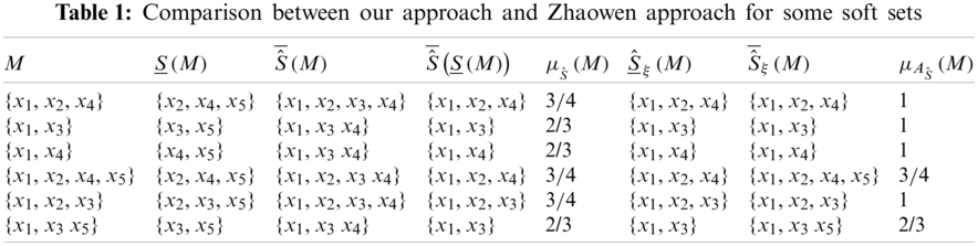
Example 3.5 From Example 3.1 Let Ŝ=(F,A) be a soft set over Ŵ and AŜ=(Ŵ,Ŝ) a soft approximation space. From this example we the following Tab. 1

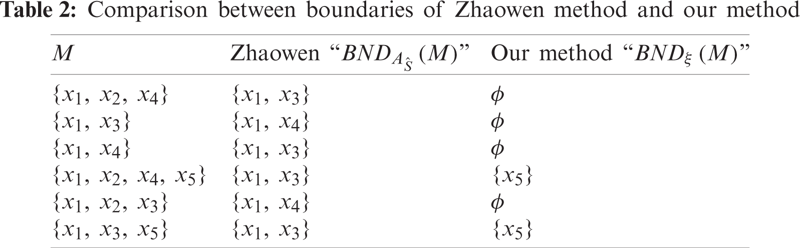
From the above Tab. 1, we deduce our method is better than Zhaowen method [15]. Also, from the above Tab. 1, we get the following Tab. 2,

Proposition 3.6 Assuming that Ŝ=(F,A) be a full soft set and AŜ=(Ŵ,Ŝ) be a soft approximation space. Subsequently, Sξ(Ŝ¯ξ(M))=Ŝ¯ξ(M),∀M⊆Ŵ.
i) Firstly, by Proposition 3.3, we get Ŝξ(Ŝ¯ξ(M))⊆Ŝ¯ξ(M),∀M⊆Ŵ. Thus, we must prove the inverse relation Ŝ¯ξ(M)⊆Ŝξ(Ŝ¯ξ(M)) as follows:
let Ŝξ(Ŝ¯ξ(M))=(M∪Ŝ¯(Ŝ(M)))∩Ŝ¯(Ŝ(M∪Ŝ¯(Ŝ(M)))⊇(M∪Ŝ¯(Ŝ(M)))∩(Ŝ(M∪Ŝ¯(Ŝ(M)))=(M∪Ŝ¯(S(M)))=Ŝ¯ξ(M) then Ŝ¯ξ(M)⊆Ŝξ(Ŝ¯ξ(M)) thus Ŝξ(Ŝ¯ξ(M))=Ŝ¯ξ(M).
Remark 3.4 Assuming that Ŝ=(F,A) be soft set over Ŵ and AŜ=(Ŵ,Ŝ) be a soft approximation space. If (F,A) is soft set then
i) Ŝ¯ξ(Mc)=(Ŝξ(M))C, for each M⊆Ŵ.
ii) Ŝξ(Mc)=(Ŝ¯ξ(M))C, for each M⊆Ŵ.
Proposition 3.7 Assuming that Ŝ=(F,A) be soft set upon Ŵ and AŜ=(Ŵ,Ŝ) be a soft approximation space. If (F,A) is soft set and keeping union and intersection, then for any M⊆Ŵ, subsequently.
i) Ŝ¯(M)⊆Ŝ¯ξ(M).
ii) Ŝ¯ξ(M)=Ŵ.
Proposition 3.8 Let Ŝ=(F,A) be soft set over Ŵ and AŜ=(Ŵ,Ŝ) be a soft approximation space. If (F,A) is partition, then for any M⊆Ŵ.
i) Ŝ(M)=Ŝξ(M).
ii) Ŝ¯ξ(M)⊆Ŝ¯(M).
Proposition 3.9 Assuming that Ŝ=(F,A) be soft set upon Ŵ while AŜ=(Ŵ,Ŝ) be a soft approximation space. If (F,A) is full soft, then for every M⊆Ŵ is soft ξ-definable if and only if Ŝ¯ξ(M)=M.
Proof
Assume that M is ξ-definable then Ŝ¯ξ(M)=Ŝξ(M)⊆M but M⊆Ŝ¯ξ(M) hence Ŝ¯ξ(M)=M, conversely, suppose that Ŝ¯ξ(M)=M this tends to Ŝ¯ξ(M)=M∪Ŝ¯(Ŝ(M))=M thus Ŝ¯ξ(M)⊆M, but Ŝξ(M)⊆M⊆Ŝ¯ξ(M)… (1). To prove that Ŝ¯ξ(M)⊆Ŝξ(M), let x∉Ŝξ(M) thus x∉M∩Ŝ¯(S(M)) this imply that x∉M or x∉Ŝ(Ŝ¯(M)) therefore x∈M∪Ŝ¯(Ŝ(M)) and hence x∉Ŝ¯ξ(M) thus Ŝ¯ξ(M)⊆Ŝξ(M)… (2), then we get from (1), (2) Ŝ¯ξ(M)=Ŝξ(M)=M. Thus M is soft ξ-definable.
4 Relationship Between Our Method and the Pawlak Approximation
In this section, we shall compare between current method and the method of Pawlak.
Definition 4.1 [15] If ℜ is equivalence relation on Ŵ define a mappings fℜ:E→P(M) by fℜ(e)=[e]ℜ for any e∈E and E=Ŵ consequently, (fℜ)E is called soft set induced by ℜ on Ŵ.
Theorem 4.1 Let Ŝ=(F,A) be soft set over Ŵ and AŜ=(Ŵ,Ŝ) be a soft approximation space. If (F,A) is partition, then for any M⊆Ŵ. Then
i) ℜ(M)=Ŝ(M)=Ŝξ(M).
ii) ℜ¯(M)=Ŝ¯(M)=Ŝ¯ξ(M).
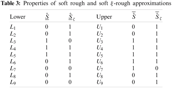
Remark 4.1 Propositions 3.1, 3.2 and 3.4 represent one of the deviations between our approach and in [15] approach. By this proposition, our approximations satisfied most of Pawlak’s properties and then Tab. 3, summarize these properties and give first comparison among our method and [15] method. We then list codes in Tab. 3 to show whether these approximations satisfy the properties (L1) to (U9). In Tab. 3, the number 1 denotes yes and 0 denotes not.

The main goal of the following results is to illustrate the relationship between soft rough approximations (that given by Wang et al. [16]) and soft pre-rough approximations (that given by our approach in the present paper).
Definition 4.2 Assuming that Ŝ=(F,A) be a full soft set upon Ŵ, AŜ=(Ŵ,Ŝ) a soft approximation space and M⊆Ŵ. Then, we define the next four main types of soft ξ-rough sets:
i) M is roughly soft ξ-definable if Ŝξ(M)≠ϕ while Ŝ¯ξ(M)≠Ŵ.
ii) M is internally soft ξ-indefinable if Ŝξ(M)=ϕ while Ŝ¯ξ(M)≠Ŵ.
iii) M is externally soft ξ-indefinable if Ŝξ(M)≠ϕ while Ŝ¯ξ(M)=Ŵ.
iv) M is totally soft ξ-indefinable if Ŝξ(M)=ϕ while Ŝ¯ξ(M)=Ŵ.
The intuitive meaning of this classification is as follows:
–-If M is roughly soft ξ-definable, this suggests that we are able to decide about some elements of Ŵ that they belong to M, and for some U elements, while, we can decide that they belong to Mc, by using the knowledge available of the soft approximation space AŜ.
–-If M is internally soft ξ-indefinable, this suggests that we are able to decide about some elements of Ŵ that they belong to Mc, but we are incapable to decide for any element of Ŵ that it belongs to M, by employing AŜ.
–-If M is externally soft ξ-indefinable, this suggests that we are able to decide about some elements of Ŵ which they belong to M, but we are incapable to decide, for any element of Ŵ that it belongs to Mc, by employing AŜ.
–-If M is totally soft ξ-indefinable, we are incapable to decide for any element of Ŵ, whether it belongs to M or Mc, by employing AŜ.
Theorem 4.2 Let AŜ=(Ŵ,Ŝ) be a soft ξ-approximation space and M⊆Ŵ. Then:
i) If M is roughly soft ξ-definable then M is roughly soft AŜ-definable.
ii) If M is internally soft ξ-definable then M is internally soft AŜ-indefinable.
iii) If M is externally soft ξ-definable then M is externally soft AŜ-indefinable.
iv) If M is totally soft ξ-indefinable then M is totally soft AŜ-indefinable.
Proof: By Proposition 3.5, the proof is obvious.
Remark 4.2 Theorem 4.2 represents a one of differences between soft rough approximations (that given by [15]) and soft ξ-rough approximations (that given by the present paper). Moreover, it illustrates the importance of our approaches in defining the sets, for example: if M is totally soft AŜ-indefinable which implies Ŝ(M)=ϕ and Ŝ¯(M)=Ŵ that is, we are incapable to decide for any element of Ŵ whether it belongs to M or Mc. But, by using soft ξ-rough approximations, Ŝξ(M)≠ϕ and Ŝ¯ξ(M)≠Ŵ and then M can be roughly soft ξ-definable Which implies that we can decide on certain elements of Ŵ which they belong to M, and this meant while for some elements of Ŵ, we able should decide that they are belong of Mc, Through using the information obtainable from the soft approximation space AŜ.