DOI:10.32604/cmc.2022.019250
| Computers, Materials & Continua DOI:10.32604/cmc.2022.019250 | |
| Article |
Human Gait Recognition: A Deep Learning and Best Feature Selection Framework
1Department of Computer Science, COMSATS University Islamabad, Wah Campus, 47080, Pakistan
2Department of Computer Science, HITEC University Taxila, Taxila, 47040, Pakistan
3College of Computer Engineering and Sciences, Prince Sattam Bin Abdulaziz University, Al-Khraj, Saudi Arabia
4Medical Convergence Research Center, Wonkwang University, Iksan, Korea
5Department of Computer Science and Engineering, Soonchunhyang University, Asan, Korea
6Department of Information Systems, Faculty of Computers and Information Sciences, Mansoura University, Mansoura, 35516, Egypt
7Department of Information Systems, Faculty of Computers and Information, Damietta University, Damietta, Egypt
*Corresponding Author: Yunyoung Nam. Email: ynam@sch.ac.kr
Received: 07 April 2021; Accepted: 10 May 2021
Abstract: Background—Human Gait Recognition (HGR) is an approach based on biometric and is being widely used for surveillance. HGR is adopted by researchers for the past several decades. Several factors are there that affect the system performance such as the walking variation due to clothes, a person carrying some luggage, variations in the view angle. Proposed—In this work, a new method is introduced to overcome different problems of HGR. A hybrid method is proposed or efficient HGR using deep learning and selection of best features. Four major steps are involved in this work-preprocessing of the video frames, manipulation of the pre-trained CNN model VGG-16 for the computation of the features, removing redundant features extracted from the CNN model, and classification. In the reduction of irrelevant features Principal Score and Kurtosis based approach is proposed named PSbK. After that, the features of PSbK are fused in one materix. Finally, this fused vector is fed to the One against All Multi Support Vector Machine (OAMSVM) classifier for the final results. Results—The system is evaluated by utilizing the CASIA B database and six angles 00°, 18°, 36°, 54°, 72°, and 90° are used and attained the accuracy of 95.80%, 96.0%, 95.90%, 96.20%, 95.60%, and 95.50%, respectively. Conclusion—The comparison with recent methods show the proposed method work better.
Keywords: Human gait recognition; deep features extraction; features fusion; features selection
The walking pattern of an individual is referred to as Gait [1]. A lot of research is being carried out on Gait at present. The analysis of human gait was started in the 1960 s [2]. At the start, the Human Gait Recognition (HGR) was used for the diagnosis of various diseases such as spinal stenosis, Parkinson's [3], and walking pattern distortion due to age factor. HGR was used to diagnose these diseases at early stages. At present, HGR is used for the recognition of a person from the walking pattern [4,5]. Plenty of techniques has been used in the past for recognition of an individual such as fingerprints, iris, retina, face recognition, ear biometrics, footprints, and recognition from the pattern of palm veins [6,7]. The method of HGR is preferable because there is no need for individual cooperation. An individual can be recognized from a distance by his/her walking style. The recent studies show that there are 24 different components of human gait that can be used to extract the feature and these features can be further used for recognition [8,9].
Massive research has been done by the researchers on the HGR. This method has been used to minimize various types of security risks, such as an embassy, bank, airport, video surveillance, and military purpose [10,11]. This method is easy to use for recognition but, several factors harshly reduce the system performance such as inferior lighting conditions, view angle changes, can be seen in Fig. 1 [12], different types of clothes [13], and different carrying conditions. A bunch of methods based on traditional features and CNN features are instituted [14].
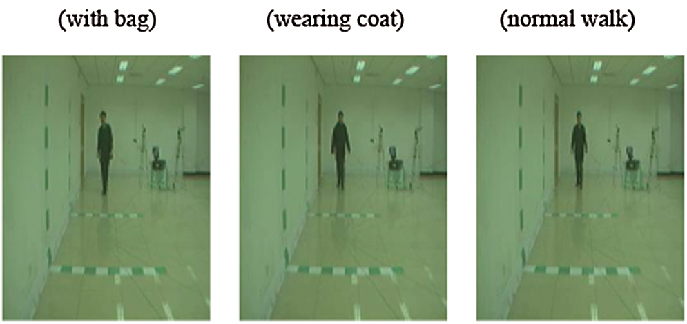
Figure 1: CASIA B sample frames [15]
HGR can be separated into two distinct groups. One group is based on a model [16] and the second group is called model free. The model-based technique uses various attributes such as joint angle. These methods are considered better for angle variations, clothing condition, and carrying conditions. A high-level model can be obtained through this approach but, the computational cost of this method is high. The model-free approach is based on the human body silhouette. This method is cost-effective but, is sensitive towards the different covariant such as angle variations, clothes, shadow, and luggage carrying conditions [17]. Therefore, the tradeoff between accuracy and computational cost should be considered. HGR is a steps process such as frames preprocessing, segmentation of region of interest, attribute computation, and finally recognition [18].
Preprocessing is a key step in Computer Vision (CV) and the computation of good attributes is based on the noiseless image [19]. This step is used for the improvement of image quality and this is achieved by eliminating the noise, contrast improvement, and background eliminating. Good features and segmentation are achieved with the help of preprocessing. Several techniques are being utilized for preprocessing of frames such as watershed, thresholding, and background removing [20].
After the process of preprocessing, the attributes of computing is a significant step [21] and is used to compute the features from image frames. The main interest is to compute the important attributes and eliminating the rest. The system efficiency is affected if there are irrelevant features. Therefore, the main concern is the extraction of relevant features only. After the computation of features, another concern is to reduce the dimensionality of these features. The feature reduction method is used to improve system efficiency by working on relevant features only and eliminating the redundant [22]. Many techniques are impelemented in literature for features reduction and selection such as entropy based selection [23], variances based reduction [24], and name a few more [25].
Plenty of research has been carried out by the researchers on HGR recently. Several techniques are applied for the recognition such as (i) HGR based on human silhouette; (ii) HGR features based on the traditional or classical methods; (iii) methods based on deep learning. The techniques based on the human silhouette are very slow and space-taking. Sometimes the incorrect silhouette gives incorrect and irrelevant attributes that affect the system reliability. The feature computation through the classical techniques is based on the low level of attributes and they are concerned with a specific problem. Therefore a fully automized system is needed for the feature computation which gives a high level of the descriptor. For the computation of high-level descriptor, a lot of techniques are offered in the literature work. There exist several problems that affect the system reliability such as various carrying conditions, clotting problems, variations in the view angles, insufficient lighting, the speed of a person, shadow of feet. These factors distort the human silhouette thus leads to inaccurate features. To address these factors the main contributions in the field of the HGR are:
a) Frames transformation based on HSV and selection of the best channel which gives the maximum features and information.
b) The computation of deep features by utilizing the VGG-16 pre-trained model with the help of transfer learning.
c) Selection of high-quality attributes with the help of a hybrid approach based on Principal Score and Kurtosis (PSaK).
d) Merging the selected attributes and fed to the One-against-All Multi SVM (OAMSVM).
Section 2 represents the related work of this study. The proposed work which includes fine-tune deep models, selection of important features, and recognition, is discussed in Section 3. Results and comparison are discussed in Section 4. The conclusion is given in Section 5.
Several techniques are used for HGR recently to recognize a person from the walking pattern. Castro et al. [26] deployed a method for HGR that is based on CNN features. In this technique, high-level descriptor learning has been done by using low-level features. To test their method, they used an HGR dataset called TUM-GAID and during experimental analysis, they reach an accuracy of 88.9%. Alotaibi et al. [27] instituted an HGR system that is based on CNN attributes. In this method, they tried to minimize the problem of occlusion that degrade system efficiency. To handle the problem of small data, they carried out augmentation of the data. Fine-tuning on the dataset is also carried out. CASIA-B database is used to assess the system performance. The 90° angle of CASIA-B dataset is used and achieved the accuracy of 98.3%, 83.87%, and 89.12% on three variations nm, bg, and cl accordingly. Li et al. [28] deployed a new network called DEEPNET in which they tried to minimize the problem that comes due to view variations. For solving this problem, they adopted the Joint Bayesian. The normalization of the gait phase is done by using Normalized Auto Correlation (NAC). After the normalization, the gait attributes are computed. For the assessment of the system, the OULP database is used and an accuracy of 89.3% is attained. Arshad et al. [4] used a method for HGR to sort out the problem of the different variations. For the computation of gait features, two CNN models VGG26 and AlexNet are used. The feature vector is computed by using entropy and Kurtosis. After computation, both vectors are fused. Fuzzy Entropy Controlled Kurtosiss (FEcK) is utilized for the selection of best features. Experimental analysis has been done on AVAMVG by achieving 99.8%, CASIA-A by achieving 99.7%, CASIA-B by achieving 93.3%, and CASIA-C by achieving 92.2% of recognition rate. To overcome the dilemma of angle variation Deng et al. [29] deployed a new HGR method. The fusion of knowledge and deterministic learning is done in this method. CASIA-B database is used for experimental analysis and 88%, 87%, and 86% recognition rate is attained on three angles 18°, 36°, and 54° accordingly.
Mehmood et al. [5] addresses the problem of variation by using a hybrid approach for feature selection. The gait attributes are computed from the image frames by using DenseNet-201. Two layers avg_pool and fc1000 are used for the computation of attributes. The parallel order method is used to merge these features. For the selection of attributes, an algorithm based on Kurtosis and firefly is used. CASIA-B is used to assess the system's performance. The accuracy of 94.3% on 18°, 93.8% on 36°, and 94.7% on 54° angle are attained, respectively. Rani et al. [30] introduced an ANN-based HGR system to identify a person from the way he walks. Image preprocessing is done background subtraction. The morphological based operation is used for tracking of image silhouette. The self-similarity-based technique is used for the assessment of the system. They evaluated the system on the CASIA dataset and observed the better performance of the system as compared to current techniques.
Zhang et al. [31] introduced a novel method to minimize the drawback of variation of clothes, angles, and carrying things. LSTM and CNN are used for the computation of attributes from RGB image frames. After that, the attributes are fused. The assessment of the system is done by using CASIA-B, FVG, and USF by achieving 81.8%, 87.8%, and 99.5% accordingly. To conquer the problem of covariations Yu et al. [32] instituted a new approach. CNN is utilized to compute the feature from the images. A Stack progressive based autoencoder is utilized to deal with the problem of variations. For reduction of features, PCA is utilized and final features are fed to the KNN algorithm. The approach is tested SZU RGB D and CASIA-B and a recognition rate of 63.90% with variations and 97% without variations were achieved. Marcin et al. [33] presented a new technique and analyzed that how different types of shoes affect the walking style of people. The total walking cycles of 2700 were analyzed obtained from 81 individuals. The accuracy of 99% was achieved on the dataset of 81 individuals. Khan et al. [34] introduced an HGR approach and used the sequence of video to compute the attributes. In this technique, a codebook is generated. After the generation of the codebook, the encoding of vector-based on fisher vector is done. CASIA-A and TUM GAID are used for assessment of the system and 100% and 97.74% recognition rate was attained, respectively.
A fully mechanized HGR system is proposed that is based on very deep features of neural networks. The proposed method is based on four steps such as: preprocessing of image frames, feature extraction through CNN model VGG-16, feature selection through a novel combined method, and at last final recognition with the help of supervised learning. The complete architecture of the system is illustrated in Fig. 2.
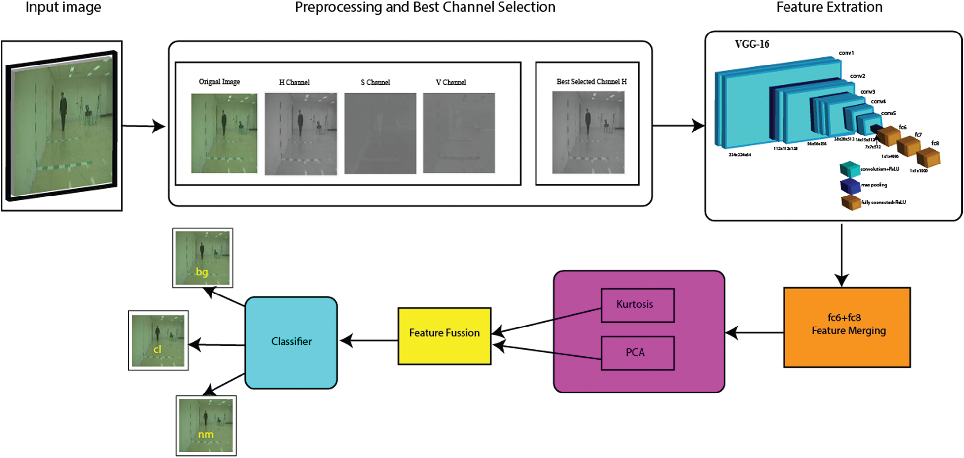
Figure 2: Proposed system architecture for HGR
Preprocessing plays an important role in CV and image processing to improve the quality of the given data [35]. Preprocessing includes, resizing of images, background removal, noise removal, and changing the color space of the image such as RGB to Gray. In this work, preprocessing is carried out to prepare data for the neural network. Initially, the image resizing is carried out. After that minimum set count based on all classes is done. Later the HSV is performed and the best channel is selected. Mathematically, HSV transformation is specified as:
The R, G, B values are divided by 255 to change the range from 0.255 to 0.1:
where,
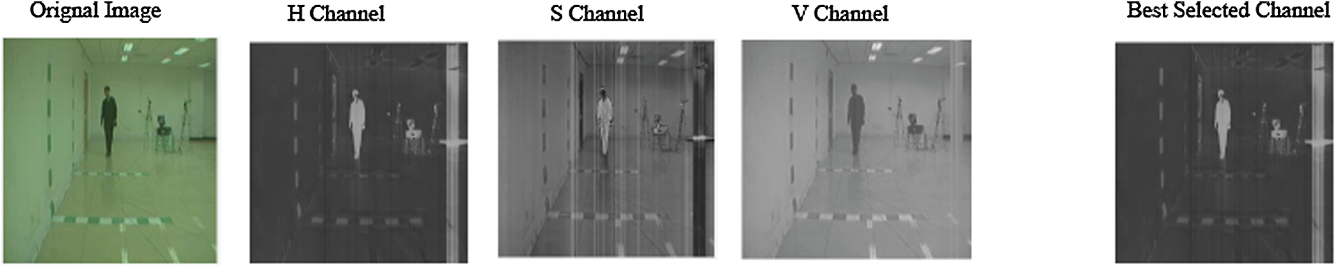
Figure 3: HSV color transformation and channel selection
3.2 Deep Learning Feature Computing
Feature computing is a very important part of machine learning and pattern recognition [36,37]. The main objective of this step the extraction of important features from the objects that are presented in the image frame. After the computation of the feature, the next step is the prediction of the object category [38]. Numerous types of features are available such as: based on geometry, shape, and texture. By utilizing these features the author tries to achieve higher accuracy but fails due to a huge dataset. Deep learning is becoming important and being used by many researchers because it works efficiently on large as well as small databases. Convolutional Neural Network (CNN) is famous types of layers-based networks that are used to extract the efficient and relevant features of the object [14]. The CNN model is based on pooling, ReLu, convolution, softmax, and fully connected (FC) layers. Low-level feature extraction is carried out by convolution layer and high-level information is obtained on FC layers.
In the proposed work, a pre-trained CNN model name VGG-16 is applied for the computation of features. The computation of features based on transfer learning is computed from the third last layer named fc6 and the second last layer named fc8. The features of both layers are combined in one matrix which proceeds in the next step. The description of each step involved in the VGG-16 model is described as follows:
VGG-16 is a famous CNN model that is being used for efficient feature computation. The size of the input image used for VGG-16 is 224 × 224 × 3. This network can be used for RGB images also. The architecture of VGG-16 is based on the input layer, 5 layers of the max pool, five segments of convolution layers having 13 layers of the total, and 3 Fully Connected (FC) layers. The filters of 3 × 3 are used in the first two convolutional layers. The filter of size 3 × 3 with stride 1 is used. A total of 64 filters are used in the first two layers and it gives an output of 224 × 224 × 64. After that, the pooling layer is used, and it gives an output of 112 × 112 × 64. After the pooling layer, two more convolution layers are used having a total 128 of filters and it gives us the output size of 112 × 112 × 128. After these convolution layers pooling layer is used, and it gives the output of size 56 × 56 × 128. After this pooling layer, two more convolution layers are added having a 256 filter. Then pooling layer is added. After that, 3 convolution layers are added having filters of 512. After this convolution layer, the pooling layer is added again. After that, 3 convolution layers are added having filters of 512. Then pooling layer is added again after these convolution layers. Finlay, the fully connected layers are added, and the final output size is 7 × 7 × 512 into the FC layer. There is a total of three FC layers. The total channels at the first two FC layers are 4096 and at the third FC layer is 1000. ReLU activation function is used in all hidden layers. The architecture of the VGG-16 is illustrated in Fig. 4.
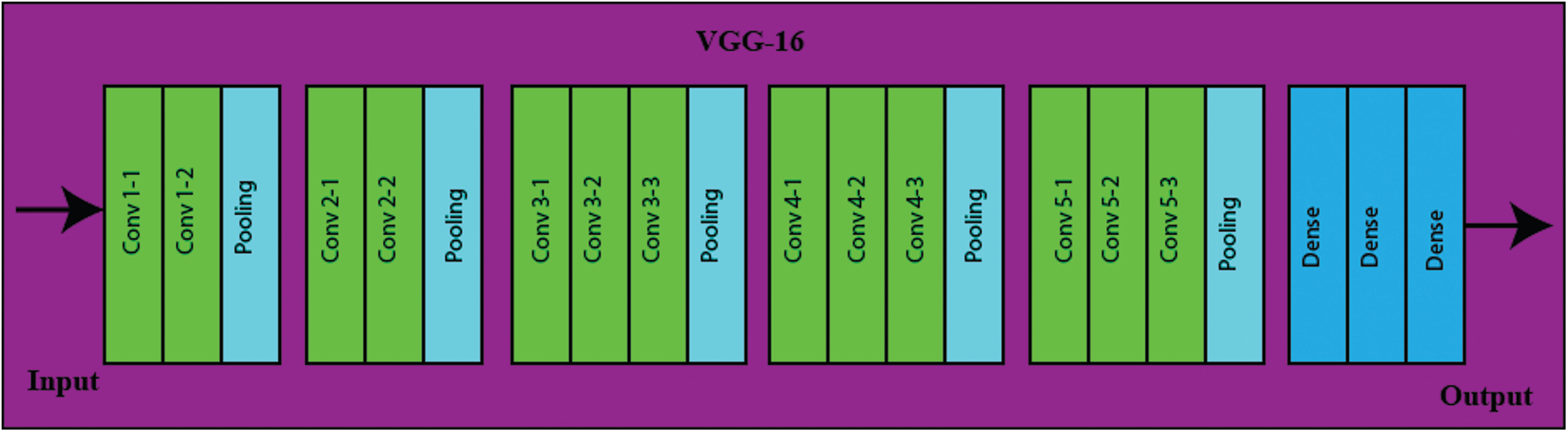
Figure 4: VGG-16 architecture
In this study, deep feature extraction is carried out by a pre-trained VGG-16CNN model. The features are computed on two layers fc6 and fc8 for the best extraction of the features. After the activation function, size of vectors N×4096 is on fc6 and N×1000 on fc8 is obtained, where N represents the number of images. After the extraction of features, the features of both layers are merged lineally.
3.2.2 Transfer Learning-Based Feature Extraction
Feature extraction is performed by transfer learning (TL) [39] on pre-trained VGG-16. For this purpose, the VGG-16 structure was trained on various angles of the HGR database CASIA-B. Activation is performed on fc6 and fc8 layers of the network and features of both the layers are merged in parallel order. The input size of the image was
Let
The maximum dimensional vector is first computed before the fusion of both vectors as shown below.
The maximum length vector is specified through this expression and a blank array is found to make both vector's length equal. This is performed by a simple subtraction operation to find the difference in the length of vectors. The mean value of maximum vector
In the above equation, the indexes of both vectors are compared and after that concatenation is performed as follows:
Feature selection is carried out by applying heuristic approach baed on Principle Score and Kurtosis to only select important features and eliminating the less important features.
Kurtosis: After feature extraction through the VGG-16 deep network, a heuristic-based approach kurtosis is applied on the computed feature vector FV. The main goal of using this approach is to select the top features and eliminating the rest. The kurtosis is formulated as:
where
Principle Component Analysis: Principal component analysis (PCA) is a statistical technique that is based on linear transformation. PCA is very useful for pattern recognition and data analysis and us is widely used in image processing and computer vision. It is used for data reduction and compression and also for decorrelation. Numerous algorithms that are neural network and multiple variation-based are being utilized as PCA on the various dataset. PCA can be defined as the transformation of
A simple formula can be generated from this concept, but it is mandatory to remember that a single input of vector
The matrix
We know that the vector
For
The rows of B are orthonormal so the inversion of PCA is conceivable as follows:
Due to these properties, PCA can be used in image processing and computer vision. In this process, a feature matrix of dimension
In this section, the proposed system validation is illustrated. The system is tested on CASIA-B [41] database that is publicly available. This database is used for Multi-view HGR. This database is based on 124 subjects of which 93 are male and 31 are female. The database is captured with the difference of 18° that is based on three different walking styles such as a person with a normal walk (nm), a person with a bag (bg), and a person in the coat (cl). Experiments are carried on six different angles of CASIA-B such as 00°, 18°, 36°, 54°, 72°, and 90° angles. All three gaits nm, bg, and cl are included in each angle. A few sample frames of 00°, 18°, 36°, 54°, 72°, and 90° angles are illustrated in Fig. 5. Six methods are used for the validation of the model including Linear SVM (L-SVM), Quadratic SVM (Q-SVM), Cubic SVM (C-SVM), Fine Gaussian SVM (F-SVM), Medium Gaussian SVM (M-SVM), and Cubic Gaussian SVM (CG-SVM). One-VS-All SVM (M-SVM) approach is utilized for the validation of the model. Statistical methods such as accuracy, Fales negative rate (FNR), precision, Area under the curve (AUC), and time are used as performance evaluation measures.
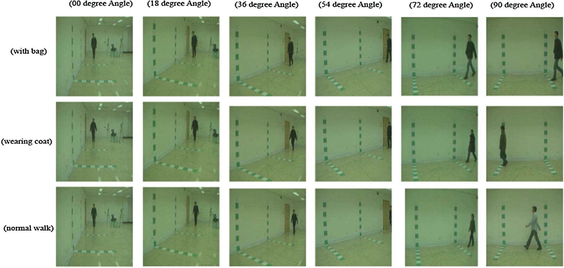
Figure 5: Sample images of CASIA B
The standard ratio of 70:30 is used for the evaluation of the system. It means that for training purposes 70% of image frames are utilized and for the testing purpose 30% of the image frames are used. The cross-validation of 10 K-Fold is used while the rate for leaning was 0.0001. Transfer Learning is used for the training and testing features computation. After the computation of features, these features along with the labels are fed into M-SVM (Linear method) for final classification. After that, the trained model is used to predict the test features. All experiments are done by using MATLAB 2018b, running on a Core i7 machine that contains 16 GB of RAM and 4 GB NVIDIA GeForce 940MX GPU. Moreover. Matcovnet, a toolbox for deep learning is used to compute deep features.
CASIA-B is a database that is publicly available and use of human gait recognition. The database was extracted in the indoor environment. There are several variations in the database such as various angles, carrying, and clothing conditions. This dataset is based on 124 subjects and this database is extracted from 11 different angles. These angles are 0°, 18°, 36°, 54°, 72°, 90°, 108°, 126°, 144°, 162°, and 180. This database was captured on 352 x 240 resolution at the rate of 25 fps. Six angles 0°, 18°, 36°, 54°, 72°, and 90° are utilized in this work. The results are computed separately and are discussed below.
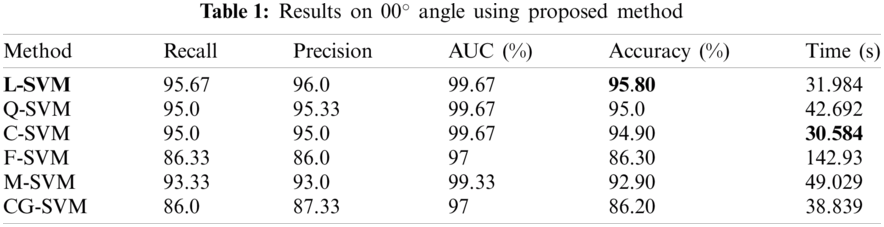
The results on 00° angle are given in this section. The results are illustrated in Tab. 1. The best accuracy is 95.80% and is achieved by L-SVM classifier. The accuracies of the rest of the classifier Q-SVM, C-SVM, F-SVM, M-SVM, and CG-SVM are 95.0%. 94.90%, 86.30%. 92.90%, and 86.20% respectively. The best results of other evaluation parameters Recall, Precision, AUC are 95.67%, 96.0%, and 99.67% are also achieved on LSVM. The Recall on rest of classifiers Q-SVM, C-SVM, F-SVM, M-SVM, and CG-SVM is 95.0%, 95.0%, 86.33%, 93.33% and 86.0% respectively. The precision of rest of classifiers Q-SVM, C-SVM, F-SVM, M-SVM, and CG-SVM is 95.33%, 95.0%, 86.0%, 93.0%, and 87.33% respectively. The AUC of the rest of the classifiers Q-SVM, C-SVM, F-SVM, M-SVM, and CG-SVM 99.67%, 99.67%, 97.0%. 99.33%, and 97.0% respectively. The computation time of the system is also calculated for all classifiers. The minimum time is 30.584 (s) in the case of C-SVM. The computational time of rest of classifiers L-SVM, Q-SVM, F-SVM, M-SVM, and CG-SVM is 31.984, 42.692, 142.93, 49.029, and 38.839 (s) respectively.
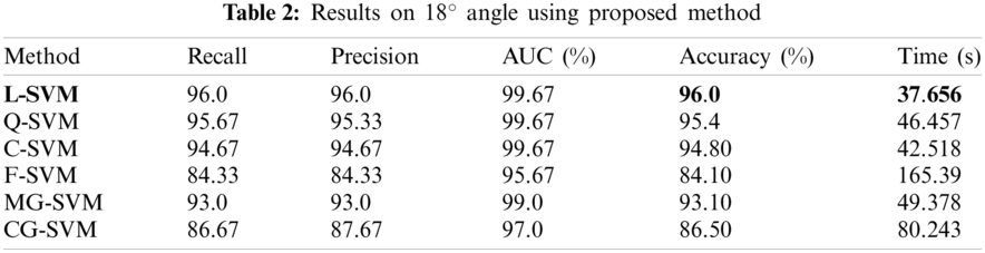
The results on 18° angle are given in this section. The results are illustrated in Tab. 2. The best accuracy is 96.0% and is achieved by L-SVM classifier. The accuracies of the rest of the classifier Q-SVM, C-SVM, F-SVM, M-SVM, and CG-SVM are 95.40%. 94.80%, 84.10%. 93.10%, and 86.50% respectively. The best results of other evaluation parameters Recall, Precision, AUC are 96.0%, 96.0%, and 99.67% are also achieved on LSVM. The Recall on the rest of classifiers Q-SVM, C-SVM, F-SVM, M-SVM, and CG-SVM is 95.67%, 94.67%, 84.33%, 93.0% and 86.67% respectively. The precision of rest of classifiers Q-SVM, C-SVM, F-SVM, M-SVM, and CG-SVM is 95.33%, 94.67%, 84.33%, 93.0%, and 87.67% respectively. The AUC of the rest of the classifiers Q-SVM, C-SVM, F-SVM, M-SVM, and CG-SVM 99.67%, 99.67%, 95.67%. 99.0%, and 97.0% respectively. The computation time of the system is also calculated for all classifiers. The minimum time is 37.656 (s) in the case of L-SVM. The computational time of rest of classifiers Q-SVM, C-SVM, F-SVM, M-SVM, and CG-SVM is 46.457, 42.518, 165.39, 49.378, and 80.243 (s) respectively.
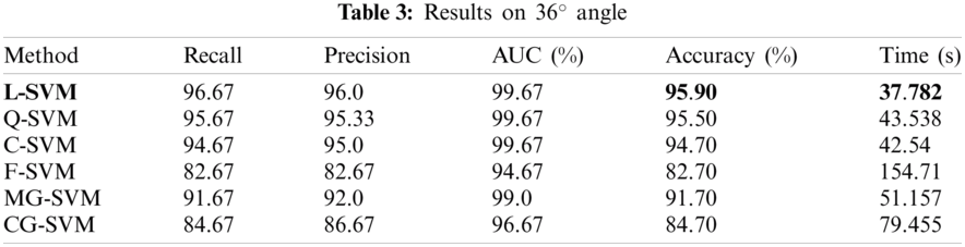
The results on 36° angle are given in this section. The results are illustrated in Tab. 3. The best accuracy is 95.90% and is achieved by L-SVM classifier. The accuracies of the rest of the classifier Q-SVM, C-SVM, F-SVM, M-SVM, and CG-SVM are 95.50%. 94.70%, 82.70%. 91.70%, and 86.70% respectively. The best results of other evaluation parameters Recall, Precision, AUC are 96.67%, 96.0%, and 99.67% are also achieved on LSVM. The Recall on the rest of classifiers Q-SVM, C-SVM, F-SVM, M-SVM, and CG-SVM is 95.67%, 94.67%, 82.67%, 91.67%, and 84.67% respectively. The precision of rest of classifiers Q-SVM, C-SVM, F-SVM, M-SVM, and CG-SVM is 95.33%, 95.0%, 82.67%, 92.0%, and 86.67% respectively. The AUC of the rest of the classifiers Q-SVM, C-SVM, F-SVM, M-SVM, and CG-SVM 99.67%, 99.67%, 94.67%. 99.0%, and 96.67% respectively. The computation time of the system is also calculated for all classifiers. The minimum time is 37.782 (s) in the case of L-SVM. The computational time of rest of classifiers Q-SVM, C-SVM, F-SVM, M-SVM, and CG-SVM is 43.538, 42.54, 154.71, 51.157, and 79.455 (s) respectively.
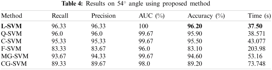
The results on the 54° angle are given in this section. The results are illustrated in Tab. 4. The best accuracy is 96.20% and is achieved by L-SVM classifier. The accuracies of the rest of the classifier Q-SVM, C-SVM, F-SVM, M-SVM, and CG-SVM are 95.90%. 95.50%, 83.10%. 94.60%, and 89.20% respectively. The best results of other evaluation parameters Recall, Precision, AUC are 96.33%, 96.33%, and 100% are also achieved on LSVM. The Recall on the rest of classifiers Q-SVM, C-SVM, F-SVM, M-SVM, and CG-SVM is 96.0%, 95.33%, 83.33%, 93.67%, and 89.33% respectively. The precision of rest of classifiers Q-SVM, C-SVM, F-SVM, M-SVM, and CG-SVM is 96.0%, 95.33%, 83.67%, 94.33%, and 89.67% respectively. The AUC of the rest of the classifiers Q-SVM, C-SVM, F-SVM, M-SVM, and CG-SVM 99.67%, 99.67%, 96.0%. 99.67%, and 98.0% respectively. The computation time of the system is also calculated for all classifiers. The minimum time is 37.50 (s) in the case of L-SVM. The computational time of rest of classifiers Q-SVM, C-SVM, F-SVM, M-SVM, and CG-SVM is 38.571, 43.077, 203.98, 53.16, and 73.748 (s) respectively.
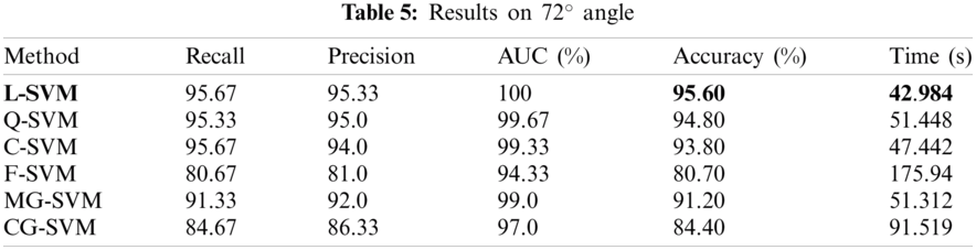
The results on 72° angle are given in this section. The results are illustrated in Tab. 5. The best accuracy is 95.60% and is achieved by L-SVM classifier. The accuracies of the rest of the classifier Q-SVM, C-SVM, F-SVM, M-SVM, and CG-SVM are 94.80%. 93.80%, 80.70%. 91.20%, and 84.40% respectively. The best results of other evaluation parameters Recall, Precision, AUC are 95.67%, 95.33%, and 100% are also achieved on LSVM. The Recall on the rest of classifiers Q-SVM, C-SVM, F-SVM, M-SVM, and CG-SVM is 95.33%, 95.67%, 80.67%, 91.33%, and 84.67% respectively. The precision of rest of classifiers Q-SVM, C-SVM, F-SVM, M-SVM, and CG-SVM is 95.0%, 94.0%, 81.0%, 92.0%, and 86.33% respectively. The AUC of the rest of the classifiers Q-SVM, C-SVM, F-SVM, M-SVM, and CG-SVM 99.67%, 99.33%, 94.33%. 99.0%, and 97.0% respectively. The computation time of the system is also calculated for all classifiers. The minimum time is 42.984 (s) in the case of L-SVM. The computational time of rest of classifiers Q-SVM, C-SVM, F-SVM, M-SVM, and CG-SVM is 51.448, 47.442, 175.94, 51.312, and 91.519 (s) respectively.
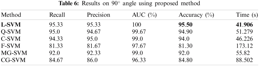
The results on 90° angle are given in this section. The results are illustrated in Tab. 6. The best accuracy is 95.50% and is achieved by L-SVM classifier. The accuracies of the rest of the classifier Q-SVM, C-SVM, F-SVM, M-SVM, and CG-SVM are 94.90%. 94.0%, 81.30%. 92.0%, and 84.80% respectively. The best results of other evaluation parameters Recall, Precision, AUC are 95.33%, 95.33%, and 100% are also achieved on LSVM. The Recall on rest of classifiers Q-SVM, C-SVM, F-SVM, M-SVM, and CG-SVM is 95.0%, 94.33%, 81.33%, 92.0%, and 84.67% respectively. The precision of rest of classifiers Q-SVM, C-SVM, F-SVM, M-SVM, and CG-SVM is 94.67%, 95.0%, 81.67%, 92.33%, and 86.0% respectively. The AUC of the rest of the classifiers Q-SVM, C-SVM, F-SVM, M-SVM, and CG-SVM 99.67%, 99.0%, 97.67%. 99.0%, and 96.33% respectively. The computation time of the system is also calculated for all classifiers. The minimum time is 41.906 (s) in the case of L-SVM. The computational time of rest of classifiers Q-SVM, C-SVM, F-SVM, M-SVM, and CG-SVM is 51.279, 46.226, 173.12, 55.82, and 88.502 (s) respectively.
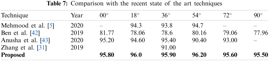
A detailed discussion is provided in this section. As demonstrated in Fig. 2, the introduced system is based on few steps such as computation of deep feature by utilizing pre-trained model of VGG-16, feature fusion, feature selection with the help of PCA and Kurtosis. After that, powerful features are selected and combined. Finally, the feature vector is fed to Multi-SVM of one against all methods. The proposed system is assessed by using six different angles of the CASIA B dataset such as 00°, 18°, 36°, 54°, 72°, and 90°. The results of the angles are calculated separately and demonstrated in Tabs. 1–6, respectively. The computational time against each angle is also computed. An extensive comparison has been carried out with the recent HGR methodologies to assess the proposed methodology as shown in Tab. 7. Mehmood et al. [5] introduced a hybrid feature selection HGR method based on deep CNN. They used the CASIA B database for the assessment for techniques and attained the recognition rate of 94.3%, 93.8%, and 94.7% on 18°, 36°, and 54° angles accordingly. Ben et al. [42] introduced an HGR technique called CBDP to address the problem of view variations. CASIA B dataset is utilized to assess the system and used CASIA-B dataset and accuracy of 81.77% on 00°, 78.06% on 18°, 78.6% on 36°, 80.16% on 54°, 79.06% on 72° and, 77.96% on 90° angles is achieved. Anusha et al. [43] advised a novel HGR method based on binary descriptors and feature dimensionality reduction is also used in the method. CASIA B dataset is utilized to assess the system performance and the accuracy of 95.20%, 94.60%, 95.40%, 90.40%, and 93.00% is attained on 00°, 18°, 36°, 54°, and 72° angles consequently. Arshad et al. [8] an HGR methodology based on binomial distribution and achieved the recognition rate of 87.70% on CASIA B using 90° angle. Zhang et al. [31] suggested an encoder-based architecture for HGR to address the problem of variations by utilizing LSTM and CNN-based networks. The system was assessed by using the CASIA B database and attained a recognition rate of 91.00% on 54°. In case of our proposed HGR method the recognition rate of 95.80%, 96.0%, 95.90%, 96.20%, 95.60%, and 95.50% is obtained on 00°, 18°, 36°, 54°, 72°, and 90° angles consequently. The strength of this work is selection of best features. The limitation of this work is less number of predictors for final classification.
HGR is a biometric-based approach in which an individual is recognized from the walking pattern. In this work, a new method is introduced for HGR to address various factors such as view variations, clothes variations, and different carrying conditions. A person wearing a coat, a person walking normally, and a person carrying a bag. In this work, the feature computation has been carried out by using pre-trained network VGG-16 instead of using classical feature methods such as color-based, shape-based, geometric-based features. A PCA and Kurtosis based method is used for the reduction of the features. Six different angles of CASIA B are utilized to assess the performance of the system and attained an average recognition rate of more than 90%, which is better than the recent techniques. The result demonstrated in this work, this can be easily verified that CNN based features give better performance in the sense of better attributes and accuracy. Deep features work well for both small datasets and as well as for large databases. Overall, the introduced approach works well for the various angles of CASIA B and gives a good performance. However, the introduced method is inefficient in the case of small data. In the future, the same approach can be applied for different angles of CASIA B and other HGR databases.
Funding Statement: This study was supported by the grants of the Korea Health Technology R & D Project through the Korea Health Industry Development Institute (KHIDI), funded by the Ministry of Health & Welfare (HI18C1216) and the Soonchunhyang University Research Fund.
Conflicts of Interest: The authors declare that they have no conflicts of interest to report regarding the present study.
1. M. Sharif, M. Z. Tahir, M. Yasmim, T. Saba and U. J. Tanik, “A machine learning method with threshold based parallel feature fusion and feature selection for automated gait recognition,” Journal of Organizational and End User Computing, vol. 32, pp. 67–92, 2020. [Google Scholar]
2. L. F. Shi, C. X. Qiu, D. J. Xin and G. X. Liu, “Gait recognition via random forests based on wearable inertial measurement unit,” Journal of Ambient Intelligence and Humanized Computing, vol. 1, pp. 1–12, 2020. [Google Scholar]
3. K. Jellinger, D. Armstrong, H. Zoghbi and A. Percy, “Neuropathology of rett syndrome,” Acta Neuropathologica, vol. 76, pp. 142–158, 1988. [Google Scholar]
4. H. Arshad, M. I. Sharif, M. Yasmin, J. M. R. Tavares, Y. D. Zhang et al., “A multilevel paradigm for deep convolutional neural network features selection with an application to human gait recognition,” Expert Systems, vol. 4, pp. e12541, 2020. [Google Scholar]
5. A. Mehmood, M. Sharif, S. A. Khan, M. Shaheen, T. Saba et al., “Prosperous human gait recognition: An end-to-end system based on pre-trained CNN features selection,” Multimedia Tools and Applications, vol. 1, pp. 1–21, 2020. [Google Scholar]
6. M. Hassaballah and S. Aly, “Face recognition: Challenges, achievements and future directions,” IET Computer Vision, vol. 9, pp. 614–626, 2015. [Google Scholar]
7. J. C. Lee, “A novel biometric system based on palm vein image,” Pattern Recognition Letters, vol. 33, pp. 1520–1528, 2012. [Google Scholar]
8. H. Arshad, M. Sharif, M. Yasmin and M. Y. Javed, “Multi-level features fusion and selection for human gait recognition: An optimized framework of Bayesian model and binomial distribution,” International Journal of Machine Learning and Cybernetics, vol. 10, pp. 3601–3618, 2019. [Google Scholar]
9. M. Zahid, F. Azam, M. Sharif, S. Kadry and J. R. Mohanty, “Pedestrian identification using motion-controlled deep neural network in real-time visual surveillance,” Soft Computing, vol. 11, pp. 1–17, 2021. [Google Scholar]
10. F. Afza, M. Sharif, S. Kadry, G. Manogaran, T. Saba et al., “A framework of human action recognition using length control features fusion and weighted entropy-variances based feature selection,” Image and Vision Computing, vol. 106, pp. 104090, 2021. [Google Scholar]
11. Y. D. Zhang, S. A. Khan, M. Attique, A. Rehman and S. Seo, “A resource conscious human action recognition framework using 26-layered deep convolutional neural network,” Multimedia Tools and Applications, vol. 8, pp. 1–23, 2020. [Google Scholar]
12. W. Kusakunniran, Q. Wu, J. Zhang and H. Li, “Gait recognition under various viewing angles based on correlated motion regression,” IEEE Transactions on Circuits and Systems for Video Technology, vol. 22, pp. 966–980, 2012 2012. [Google Scholar]
13. X. Li, Y. Makihara, C. Xu, Y. Yagi and M. Ren, “Joint intensity transformer network for gait recognition robust against clothing and carrying status,” IEEE Transactions on Information Forensics and Security, vol. 14, pp. 3102–3115, 2019. [Google Scholar]
14. N. Hussain, M. Sharif, S. A. Khan, A. A. Albesher, T. Saba et al., “A deep neural network and classical features based scheme for objects recognition: An application for machine inspection,” Multimedia Tools and Applications, vol. 1, pp. 1–23, 2020. [Google Scholar]
15. S. Zheng, J. Zhang, K. Huang and T. Tan, “Robust view transformation model for gait recognition,” in 2011 18th IEEE Int. Conf. on Image Processing, NY, USA, pp. 2073–2076, 2011. [Google Scholar]
16. F. Tafazzoli and R. Safabakhsh, “Model-based human gait recognition using leg and arm movements,” Engineering Applications of Artificial Intelligence, vol. 23, pp. 1237–1246, 2010. [Google Scholar]
17. Z. Wu, Y. Huang, L. Wang, X. Wang and T. Tan, “A comprehensive study on cross-view gait based human identification with deep cnns,” IEEE Transactions on Pattern Analysis and Machine Intelligence, vol. 39, pp. 209–226, 2016. [Google Scholar]
18. M. Hassaballah, H. A. Alshazly and A. A. Ali, “Ear recognition using local binary patterns: A comparative experimental study,” Expert Systems with Applications, vol. 118, pp. 182–200, 2019. [Google Scholar]
19. A. Majid, M. Yasmin, A. Rehman, A. Yousafzai and U. Tariq, “Classification of stomach infections: A paradigm of convolutional neural network along with classical features fusion and selection,” Microscopy Research and Technique, vol. 83, pp. 562–576, 2020. [Google Scholar]
20. M. Piccardi, “Background subtraction techniques: A review,” in 2004 IEEE Int. Conf. on Systems, Man and Cybernetics, NY, USA, pp. 3099–3104, 2004. [Google Scholar]
21. M. A. Khan, T. Akram, N. Muhammad, M. Y. Javed and S. R. Naqvi, “Improved strategy for human action recognition; experiencing a cascaded design,” IET Image Processing, vol. 14, pp. 818–829, 2019. [Google Scholar]
22. M. S. Sarfraz, M. Alhaisoni, A. A. Albesher, S. Wang and I. Ashraf, “Stomachnet: Optimal deep learning features fusion for stomach abnormalities classification,” IEEE Access, vol. 8, pp. 197969–197981, 2020. [Google Scholar]
23. A. Adeel, T. Akram, A. Sharif, M. Yasmin, T. Saba et al., “Entropy-controlled deep features selection framework for grape leaf diseases recognition,” Expert Systems, vol. 11, pp. 1–21, 2020. [Google Scholar]
24. M. B. Tahir, K. Javed, S. Kadry, Y. D. Zhang, T. Akram et al., “Recognition of apple leaf diseases using deep learning and variances-controlled features reduction,” Microprocessors and Microsystems, vol. 1, pp. 104027, 2021. [Google Scholar]
25. S. Kadry, Y. D. Zhang, T. Akram, M. Sharif, A. Rehman et al., “Prediction of COVID-19-pneumonia based on selected deep features and one class kernel extreme learning machine,” Computers & Electrical Engineering, vol. 90, pp. 106960, 2021. [Google Scholar]
26. F. M. Castro, M. J. Marín-Jiménez, N. Guil and N. Pérez de la Blanca, “Automatic learning of gait signatures for people identification,” Journal of Computational Intelligence, vol. 10306, pp. 257–270, 2017. [Google Scholar]
27. M. Alotaibi and A. Mahmood, “Improved gait recognition based on specialized deep convolutional neural network,” Computer Vision and Image Understanding, vol. 164, pp. 103–110, 2017. [Google Scholar]
28. C. Li, X. Min, S. Sun, W. Lin and Z. Tang, “Deepgait: A learning deep convolutional representation for view-invariant gait recognition using joint Bayesian,” Applied Sciences, vol. 7, pp. 210, 2017. [Google Scholar]
29. M. Deng, T. Fan, J. Cao, S. Y. Fung and J. Zhang, “Human gait recognition based on deterministic learning and knowledge fusion through multiple walking views,” Journal of the Franklin Institute, vol. 357, pp. 2471–2491, 2020. [Google Scholar]
30. M. P. Rani and G. Arumugam, “An efficient gait recognition system for human identification using modified ICA,” International Journal of Computer Science and Information Technology, vol. 2, pp. 55–67, 2010. [Google Scholar]
31. Z. Zhang, L. Tran, X. Yin, Y. Atoum, J. Wan et al., “Gait recognition via disentangled representation learning,” in Proc. of the IEEE/CVF Conf. on Computer Vision and Pattern Recognition, NY, USA, pp. 4710–4719, 2019. [Google Scholar]
32. S. Yu, H. Chen, Q. Wang, L. Shen and Y. Huang, “Invariant feature extraction for gait recognition using only one uniform model,” Neurocomputing, vol. 239, pp. 81–93, 2017. [Google Scholar]
33. D. Marcin, “Human gait recognition based on ground reaction forces in case of sport shoes and high heels,” in 2017 IEEE Int. Conf. on INnovations in Intelligent SysTems and Applications, NY, USA, pp. 247–252, 2017. [Google Scholar]
34. M. H. Khan, F. Li, M. S. Farid and M. Grzegorzek, “Gait recognition using motion trajectory analysis,” in Int. Conf. on Computer Recognition Systems, Lag Vegas, USA, pp. 73–82, 2017. [Google Scholar]
35. M. I. Sharif, M. Alhussein, K. Aurangzeb and M. Raza, “A decision support system for multimodal brain tumor classification using deep learning,” Complex & Intelligent Systems, vol. 2, pp. 1–14, 2021. [Google Scholar]
36. T. Akram, Y. D. Zhang and M. Sharif, “Attributes based skin lesion detection and recognition: A mask RCNN and transfer learning-based deep learning framework,” Pattern Recognition Letters, vol. 143, pp. 58–66, 2021. [Google Scholar]
37. H. T. Rauf, M. I. U. Lali, S. Kadry, H. Alolaiyan, A. Razaq et al., “Time series forecasting of COVID-19 transmission in Asia pacific countries using deep neural networks,” Personal and Ubiquitous Computing, vol. 1, pp. 1–18, 2021. [Google Scholar]
38. M. Rashid, M. Alhaisoni, S. H. Wang, S. R. Naqvi, A. Rehman et al., “A sustainable deep learning framework for object recognition using multi-layers deep features fusion and selection,” Sustainability, vol. 12, pp. 5037, 2020. [Google Scholar]
39. H. C. Shin, H. R. Roth, M. Gao, L. Lu, Z. Xu et al., “Deep convolutional neural networks for computer-aided detection: CNN architectures, dataset characteristics and transfer learning,” IEEE Transactions on Medical Imaging, vol. 35, pp. 1285–1298, 2016. [Google Scholar]
40. Y. Liu and Y. F. Zheng, “One-against-all multi-class SVM classification using reliability measures,” in IEEE Int. Joint Conf. on Neural Networks, NY, USA, pp. 849–854, 2005. [Google Scholar]
41. M. Goffredo, J. N. Carter and M. S. Nixon, “Front-view gait recognition,” in IEEE Second Int. Conf. on Biometrics: Theory, Applications and Systems, NY, USA, pp. 1–6, 2008. [Google Scholar]
42. X. Ben, C. Gong, P. Zhang, R. Yan and W. Meng, “Coupled bilinear discriminant projection for cross-view gait recognition,” IEEE Transactions on Circuits and Systems for Video Technology, vol. 30, pp. 734–747, 2019. [Google Scholar]
43. R. Anusha and C. Jaidhar, “Clothing invariant human gait recognition using modified local optimal oriented pattern binary descriptor,” Multimedia Tools and Applications, vol. 79, pp. 2873–2896, 2020. [Google Scholar]
 | This work is licensed under a Creative Commons Attribution 4.0 International License, which permits unrestricted use, distribution, and reproduction in any medium, provided the original work is properly cited. |