Computers, Materials & Continua DOI:10.32604/cmc.2022.019019
Article

A Modified Search and Rescue Optimization Based Node Localization Technique in WSN

Suma Sira Jacob1,*, K. Muthumayil2, M. Kavitha3, Lijo Jacob Varghese4, M. Ilayaraja5, Irina V. Pustokhina6 and Denis A. Pustokhin7

1Department of Computer Science and Engineering, Christian College of Engineering and Technology, Oddanchatram, 624619, India
2Department of Information Technology, PSNA College of Engineering and Technology, Dindigul, 624622, India
3Department of Electronics and Communication Engineering, K. Ramakrishnan College of Technology, Tiruchirappalli, 621112, India
4Department of Electrical and Electronics Engineering, Christian College of Engineering and Technology, Oddanchatram, 624619, India
5School of Computing, Kalasalingam Academy of Research and Education, Krishnankoil, 626128, India
6Department of Entrepreneurship and Logistics, Plekhanov Russian University of Economics, Moscow, 117997, Russia
7Department of Logistics, State University of Management, Moscow, 109542, Russia
*Corresponding Author: Suma Sira Jacob. Email: sumasarajaco@gmail.com
Received: 19 March 2021; Accepted: 20 April 2021

Abstract: Wireless sensor network (WSN) is an emerging technology which find useful in several application areas such as healthcare, environmental monitoring, border surveillance, etc. Several issues that exist in the designing of WSN are node localization, coverage, energy efficiency, security, and so on. In spite of the issues, node localization is considered an important issue, which intends to calculate the coordinate points of unknown nodes with the assistance of anchors. The efficiency of the WSN can be considerably influenced by the node localization accuracy. Therefore, this paper presents a modified search and rescue optimization based node localization technique (MSRO-NLT) for WSN. The major aim of the MSRO-NLT technique is to determine the positioning of the unknown nodes in the WSN. Since the traditional search and rescue optimization (SRO) algorithm suffers from the local optima problem with an increase in number of iterations, MSRO algorithm is developed by the incorporation of chaotic maps to improvise the diversity of the technique. The application of the concept of chaotic map to the characteristics of the traditional SRO algorithm helps to achieve better exploration ability of the MSRO algorithm. In order to validate the effective node localization performance of the MSRO-NLT algorithm, a set of simulations were performed to highlight the supremacy of the presented model. A detailed comparative results analysis showcased the betterment of the MSRO-NLT technique over the other compared methods in terms of different measures.

Keywords: Node localization; WSN; chaotic map; search and rescue optimization algorithm; localization error

1  Introduction

Wireless sensor network (WSN) is a developing technology which has significant applicability in several areas such as surveillance, healthcare, astronomy, agriculture, and military [1]. It has extensive application opportunities because of its easier and fast installation, and self-organization. It contains a larger number of small sized and, cheap independent sensor nodes (i.e., homogenous/heterogeneous) to monitor the environmental and physical circumstances [2]. This independent node performs sensing, processing, and sending the collected information from the atmosphere to the base station (BS) [3]. The distinct biological, chemical, optical, magnetic sensor nodes are attached to the nodes to calculate atmospheric features. The characteristics of WSN such as self-organizing and fast placement make it favorable for all the applications of WSN. In WSN applications, the sensors observe and transmit the event of interest that is investigated while the location of targeted node reported the event is known. The computation of the sensor node is a significant issue of the WSN and is termed a localization problem [4]. Fig. 1 shows the structure of WSN.

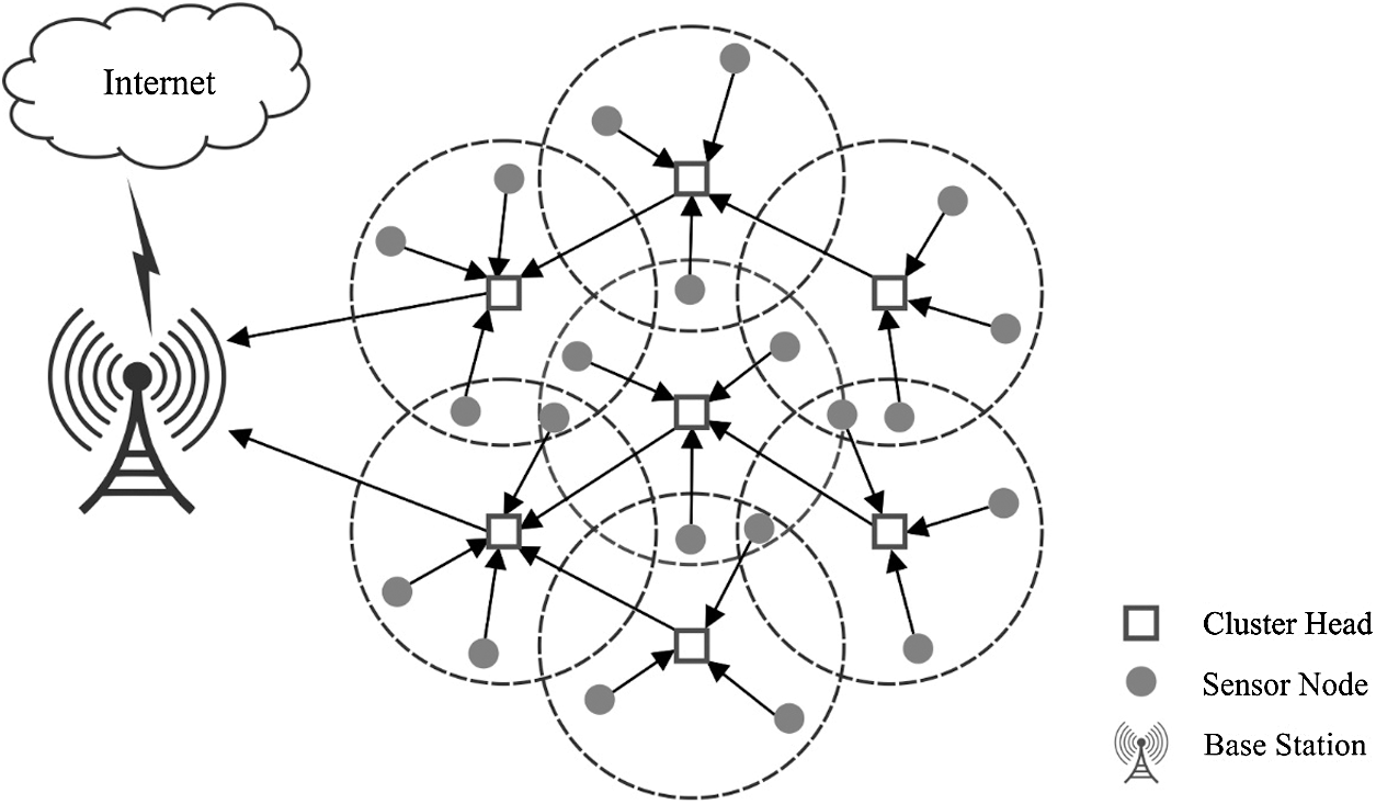
Figure 1: The architecture of WSN

Node localization (NL) technique can localize and trace the nodes; therefore, the observing data find more useful. The information is collected at the BS would be useless to the client without the localization data of the nodes in the target area [5]. The localization is determined as the computation of the location of unknown sensors termed as targeted node by the use of anchor nodes, which is depending upon the measurements like angle of arrival, time of arrival, maximal likelihood, triangulation, and time variance of arrival, etc. [6]. The localization problem of WSN is solved by utilizing the Global Positioning Systems (GPS) with all sensor nodes, however, this is not preferred because of the cost, size, and energy problems. Thus, an effective and enhanced alternate solution is needed for localizing the sensor nodes. Several nonGPS based localization systems are utilized, which are classified as range free and range based techniques [7]. The range based localization method utilizes point-to-point distance or angle based calculations among sensors. The range free localization system doesn't need range data among targeted and sensor nodes; however, it is based on topological data. The range based method gives additional accuracy than range free localization techniques, but they have not been so economical [8]. In recent times, the NL in WSNs is managed as a multidimensional and multi-modal optimization problem that can be resolved by population based stochastic methods. Several metaheuristic methods are applied to resolve the localization problem in WSNs. These methods have achieved reduced localization error in significant manner. They have tried to resolve an optimization problem by error and trial where the possible outcomes process and closest optimum solution is recognized. Presently, several optimization methods like cuckoo search (CS), butterfly optimization algorithm (BOA), gravitational search algorithm (GSA), particle swarm optimization (PSO), artificial bee colony (ABC), genetic algorithm (GA), etc. are applied efficiently in determining the locations of unknown node in the WSNs [9].

This paper designs a modified search and rescue optimization based node localization technique (MSRO-NLT) for WSN. The MSRO-NLT technique intends to computation the positioning of the unknown nodes that exist in the WSN. As the classical search and rescue optimization (SRO) algorithm suffers from the local optima problem, MSRO algorithm is derived by incorporating the concept of chaotic maps into the SRO algorithm to enhance the diversity. For assessing the proficient node localization results of the MSRO-NLT algorithm, a series of simulations were performed to showcase the improved localization performance of the MSRO-NLT technique.

2  Literature Review

Various metaheuristic techniques have been implemented for enhancing the localization technique to raise the accuracy of actual localization method. Singh et al. [10] employed an enhanced method for localization and later, utilized PSO method to determine the outcomes. Zhao et al. [11] presented a localization technique depending upon hybrid chaotic approach. Cui et al. [12] enhanced the value of hop count with the values of general 1-hop node among nearby nodes and transformed the discrete hop count value to additionally precise continuous value. The Differential Evolution (DE) method is presented to attain the optimum global result which is equivalent to the calculated position of unknown node while it makes huge time overhead and consumes power when enhancing the localization accuracy.

A butterfly optimization technique is unitized for localizing the sensors in WSN [13]. The projected localization system has been authenticated by distinct node counts with distance measurement are degraded by the Gaussian noise. Ahmed et al. [14] have proposed an NL method depending upon Whale Optimization Algorithm (WOA) is the major purpose for localizing sensor nodes in WSNs precisely. A hybrid localization method is presented in [15] depending upon DE and Dynamic Weight Particle Swarm Optimization (DWPSO) techniques. The researchers observe that reducing the square error of calculated and measured distance can reduce the localization error.

To accomplish NL, Strumberger et al. [16] presented a model in which the Elephant Herding Optimization (EHO) and tree growth method based swarm intelligence metaheuristics are utilized to resolve the WSN localization problems. To determine the enhancement, practical investigates are carried out in varied sizes of WSN ranging from 25–150 targeted nodes where the distance measurement are degraded by the Gaussian noise. Cui et al. [17] proposed a localization method, which is combined with Niching PSO and trustworthy reference node chosen to resolve the problems. At the initial stage, the proposed method selects the stable neighboring localized nodes as a reference in the localization. By the application of the niching technique, the localization ambiguity problem leads to collinear anchors. For another issue, the method employs three criteria for choosing a lesser group of stable neighboring anchors to localize unknown nodes. The tree conditions are given for choosing trustworthy neighborhood anchors whereas the unknown node is localized, like angle, distance, and localization accuracy.

In Rajakumar et al. [18], a GWO method is embedded for indicating the precise position of unknown nodes, and later it manages the NL issue. The established task is performed with the application of MATLAB whereas nodes are located arbitrarily within the targeted region. The features like ratio of localized node, processing time, and lower localization error value are employed to examine the capability of the GWO rules. Gumaida and Luo [19] displayed an advanced and high efficiency method that is based on the new technique for localization process in an outside environment. The novel optimization method focuses on PSO with Variable Neighborhood Search (VNS) and named hybrid PSO with VNS (HPSOVNS). The objective function is employed by HPSOVNS for the optimization of the last mean squared range error of nearby anchor nodes.

Li et al. [20] projected a method to improvise the accurateness of mobile NL in coal mines and to remove the effect with drive direction offsets, which are utilized positioning methods. A ranging technique is investigated inside a probabilistic method. Recently introduced localization technique based on overlapping self adjustable rule, and the anchor is selected. A minimum cost fully distributed WSN localization technique with optimum accuracy has been presented in [21]. DCRL-WSN displays a ball shaped extended bound for the inaccurate identified location of the targeted nodes. Moreover, a new certain condition for estimating is provided to the targeted node, in the application of this criterion, and expanded bound of targeted nodes are decreased. However, a group of NL techniques has been presented in the survey, yet there is a need to emerging a novel technique to improve the localization rate with lesser error.

3  The Proposed MSRO-NLT Technique

The proposed MSRO-NLT algorithm performs NL by following a series of steps, as given in Fig. 2. Initially, the nodes are randomly deployed in the interested region. Then, the node initialization process takes place and neighboring nodes interact with one another for information sharing. Followed by, the MSRO-NLT technique is applied to determine the positioning of the target nodes. A detailed description of the MSRO-NLT technique is provided in the succeeding subsections.

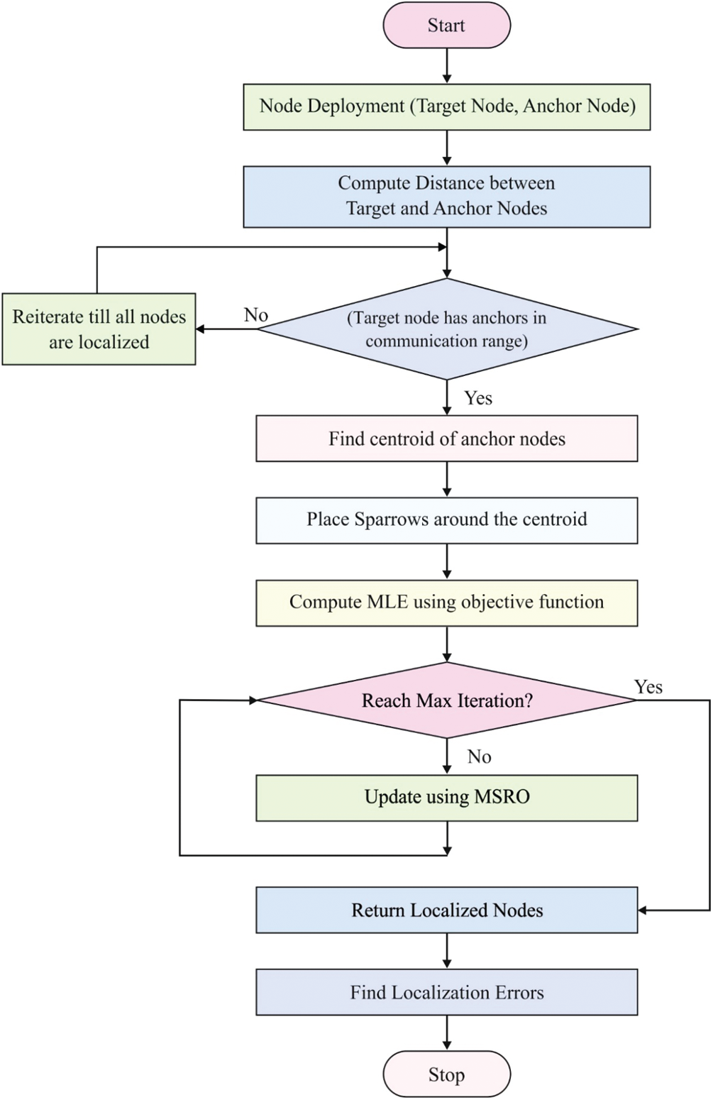
Figure 2: The workflow of proposed model

3.1 Problem Formulation

The aim of NL in WSN is the calculation of the position of unknown target sensors node which is arbitrarily distributed in the observing atmosphere through the objective of minimizing the objective function.

The estimate of unknown node location is determined with range based distributed localized model that is carried out in 2 stages: the ranging as well as position estimation stages. In order to assess the distance among target as well as anchor nodes from the initial phase, the intensity of the received signal is assumed. Because of the details that the signal is affected by Gaussian noise, accurate measurement cannot be achieved. During the next stage, the coordinates of target nodes are evaluated by utilizing geometrical manner, trilateration model [16]. The position estimation stage utilizes the before reached data in the ranging stage. Distinct ways are existed to determine the positions of the target node that exists, but a specific problem statement, the trilateration model is employed. Because of the measurement imprecision in these 2 stages, swarm intelligence (SI) technique is applied for minimizing the localized error. In 2D WSN observing atmosphere, M refers the target nodes and N represents the anchors are arbitrarily utilized by the communication range R. To estimate the distance among every target as well as anchors are revised by Gaussian noise variable.

For all target nodes, the distance amongst anchor nodes from their range is computed by utilizing formula d^i=di+ni, where ni implies an additive Gaussian noise, and di denotes the actual distance which is evaluated by utilizing the Eq. (1):

di=(x−xi)2+(y−yi)2,(1)

where the position of target nodes is represented as (x,y), and the coordinates of anchor node is demonstrated as (xi,yi). The variance of ni, as noise which affects the evaluated distance amongst target as well as anchor nodes are provided in Eq. (2):

σd2=β2⋅Pn.dj,(2)

where Pn refers the percentage noise from distance measurement di±dj(Pn100  ), and β implies the parameter whose value is generally set to 0.1 in real time scenarios.

During the trilateration model to estimate the coordinates of unknown sensor nodes, the unknown node is determined as localization when there are lesser 3 anchor nodes with known positions A(xa,ya), B(xb,yb), and C(xc,yc), within their communication range R, and distance di in target node n. By employing the trigonometric rules of sines and cosines, the coordinates of target node are computed. It minimizes the error among actual as well as predictable distances.

3.2 Design of MSRO Algorithm

The scientific method of the projected technique to resolve a “maximization problem” is defined. In SRO algorithm, the human location is equivalent to the solution of the optimization issue, and the quantity of clues obtain in these locations denotes the objective function for this solution.

3.2.1 Clues

The member of a group collects clue data in the search. Some of the clues are left in case of obtaining optimum clues in other locations, however, the data over them are utilized to enhance the searching process [22]. In this method, the left clues position is saved in the memory matrix (matrix M), whereas the human position is saved in the position matrix (matrix X). The dimension of matrix M is equivalent to these matrix X. They are N×D matrices, in which D represents dimension of the problem and N denotes human count. The clues matrix comprises the position of obtained clues. This matrix contains 2 matrices X and M. Eq. (1) displays the creation of C. Every novel solution in individual and social stages is made depending upon clues matrix, and it is a major role of SRO. The matrix X, M, and C are upgraded in all human search stages:

C={XM}  ={X11⋯X1D⋮⋱⋮XN1⋯XNDM11⋯M1D⋮⋱⋮MN1⋯MND},(3)

where M and X represents memory and human location matrices, correspondingly, and XN1 denotes position of first dimension for the Nth human. Also, M1D represent location of the Dth dimension for the first memory.

3.2.2 Social Phase

Assuming the description provided in the earlier segment, and an arbitrary clue between obtained clues, the searching direction can be defined as:

SDi=(Xi−Ck)  ,  k≠i,(4)

where Xi, Ck, and SDi represents position of jth human, the location of the kth clue, and search direction of jth  human, correspondingly. k indicates arbitrary integer number range among 1 and 2N and selected in a manner k≠i. It is significant to highlight that humans usually search in this manner that every desirable area is searched and some repetitive position cannot search again. Thus, the search must be made in a way in which motion of group members to one another is restricted. Therefore, each dimension of Xj cannot be adjusted by movement in the direction of Eq. (4). For applying these limitations, the binomial crossover operator has been utilized. When the assumed clue is greater than the clue relevant to the present location, an area nearby SDj direction and the location of that searched clue; or else, the searching process would endure nearby the present position beside the SDi direction. Lastly, the succeeding formula is utilized for the social stage:

Xi,j=′{{Ck,j+rl×(Xi,j−Ck,j),  if  f(Ck)>,f(Xi)Xi,j+rl×(Xi,j−Ck,j),  otherwiseXi,j  if  r2<SEor  j=jrand,otherwise,(j=1,  …,  D),  (5)

where Xi,j′ represents novel location of jth dimension of ithhuman; Ck,  j demotes location of jth dimension for the kth obtained clue; f(Ck) and f(Xi) represents objective function value for the solution Ck and Xi, correspondingly; rl and r2 denotes arbitrary number; jrand indicates arbitrary integer number range among 1 and D that guarantees that as a minimum of 1D of Xi,j′ is distinct from Xi,j; and SE is a technique variable range between 0 and 1. Eq. (5) is utilized to attain a novel location of the jth human in every dimension.

3.2.3 Individual Phase

In individual phase, human search nearby their present location, and the concept of linking distinct clues are utilized in the social stage is employed to search. Conflicting to the social stage, every dimension of Xi altered in the separation stage. The novel location of jth human is attained by:

Xi′=Xj+r3×(Ck−Cm)  ,  i≠k≠m,(6)

where k and m represent arbitrary integer number range among 1 and 2N. For preventing motion besides another clues, k and m are selected in this manner that i≠k≠m. r3 indicates an arbitrary number with uniform distribution range among [0, 1].

3.2.4 Boundary Control

In all metaheuristic techniques, each solution must be positioned in the solutions space, and when they are away from permissible solution space, they must be changed. In case the novel location of human is away from solution space, the succeeding formula is utilized to change the novel location:

Xi,j=′{(Xi,j+Xj max  )2,  if  Xi,j′>xjmax,(Xi,j+Xj min  )2,  if  Xi,j′<xjmin,  (j=1,…,  D)(7)

where Xjmax   and Xjmin represents value of the minimum and maximum threshold for the jth dimensions, correspondingly.

3.2.5 Update Information and Position

In all iterations, the group member would search based on these 2 stages, and afterward all stages, when the values of objective function in location Xi′(f(Xi)) is higher than the prior one (f  (Xi)), the earlier location (Xi) would be saved in an arbitrary location of memory matrix (M) by Eq. (8) and this location would be adopted as a novel location by Eq. (9). Or else, this location is left and memory is not upgraded:

Mn={Xi,if  f(Xi′)>,f(Xi)  Mn, otherwise  (8)

Xi={Xi′,  if  f(Xi′)>,f(Xi)  Xi, otherwise,  (9)

where Mn represents position of nth clue stored in the memory matrix and n denotes arbitrary integer number range among 1 and N. By this kind of memory, upgrading raises the variety of the method and the capability of technique to detect the global optimal solution.

3.2.6 Abandoning Clues

During the searching and rescuing processes, time is significant feature as the missing patients might be wounded and the delayed of search and rescue groups might lead to mortality. Thus, these processes should be made in a manner that the large space is searched in the short probable time. Therefore, when a human could not detect optimum clues afterward a specific search counts nearby their present location, he/she left the present location and refer to a novel location. To design this nature, initially, unsuccessful search number (USN) is fixed to zero for every human being. When the human detects optimum clue in the 1st or 2nd stage of the searching process, the USN is fixed to zero for this human; or else, it would raise by one point is denoted by:

USNi=  {USNi+l,  if  f(Xi′)<,f(Xj)0,otherwise  (10)

The arbitrary location in the search space can be represented by Eq. (11), and the USNi is fixed to zero for that human:

Xi,j=Xjmin  +r4×(Xjmax−Xj min  )j=1,  …, D,(11)

where r4 represents arbitrary number and it is distinct for every dimension. Fig. 3 illustrates the flowchart of SRO technique. The MSRO algorithm is based on the concepts of SRO algorithm and chaotic map. Though SRO exhibits improved efficiency over PSO and GA, it suffers from local optima issue [23]. For defining SD, the normalization range is minimized proportionally to the iteration and is provided by.

v(t)=MAX---  tT(MAX−MIN)(12)

where T indicates the highest number of iterations, f is the present iteration,  [MAX,MIN]  denotes the adaptive interval.

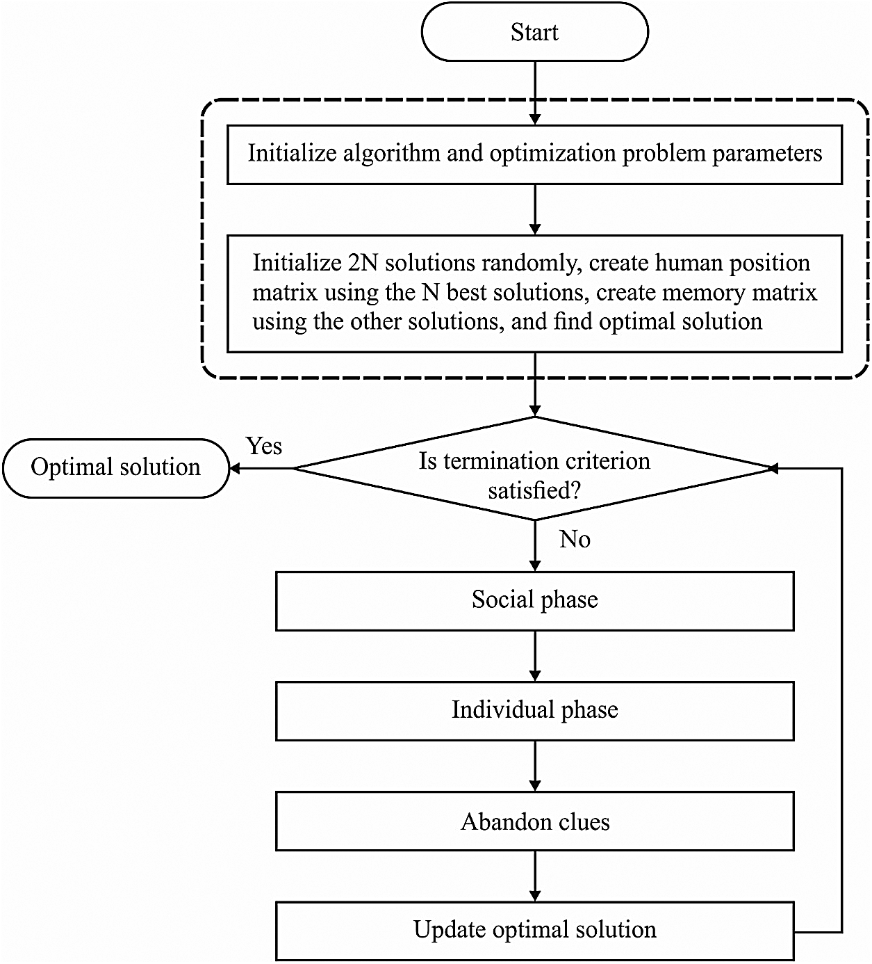
Figure 3: The flowchart of SRO algorithm

Normalization of Ck(t) take place from [a,  b] to [0,\,v(t)], as given below.

Cknorm(t)=(Ck(t)−a)×(V(t)−0)(b−a)(13)

where k denotes the index of chaotic maps, f is the present round, and [a,  b] depicts the range of chaotic maps. It is shown that the [a,  b] can be mapped to [0,  v(t)] at every round whereas v(t) gets reduced with iterations. The chaotic maps chosen are given below.

3.3 Processes Involved in MSRO-NLT Technique

The MSRO-NLT localization technique is mainly employed to estimate the coordinate points of the sensors in WSN. The aim is to determine the coordinate points of the target nodes with the minimization of objective function. The processes involved in the MSRO-NLT technique are given in the following

i)   Initialization of N unknown nodes and M anchor nodes randomly in the sensing field with the transmission radius R. Every anchor node determines the positioning and sends the coordinate points to the nearby nodes. For every iteration, the node that settles down at the end is called a reference node and it plays as anchor node in the subsequent iterations.

ii)   A set of three or greater than three anchor nodes present in the transmission radius of a node is treated as a localized node.

iii)   The distance between the target and anchor nodes is determined and gets modified using additive Gaussian noise. The target node computes the distance with d^i=di+ni where di denotes the actual distance which is determined between the positions of the target node (x,  y) and location of beacon (xi,yi) using Eq. (14):

di=(x−xi)2+(y−yi)2(14)

iv)    The target node is called a localizable node if it includes three anchor nodes within the transmission range of the target node. Based on the utilization of the trigonometric laws of sine or cosine, the coordinate points of the target nodes can be computed.

v)    The MSRO-NLT approach is employed for determining the coordinate points (x,y) of the target node that minimizes the localization error. The primitive utilized in the localization issue is an average square distance between the target and anchor nodes which has been minimized using Eq. (15):

f(x,y)=1N(∑i=1N⁡(x−xi)2+(y−yi)2−d^)2(15)

vi)    The optimum measure (x,y) is computed by the use of MSRO-NLT model at the end of the iteration.

vii)    The total localization error is computed next to the estimation of the localizable target node NL. It is validated evaluated as an average square of distance from determined node coordinate points (Xi,Yi) whereas the original node coordinate points (xi,yi) are defined by:

EL=1N1∑i=1N⁡(xi−Xi)2+(yi−Yi)2(16)

viii)    Steps 2–5 get iterated till the location of the target nodes is identified. The localization model is based on the high localization error E1 and unlocalized node count NNL which is computed by the use of NNL=M−NL. The least score of E1 and NNL results in proficient localization performance.

4  Experimental Validation

4.1 Implementation Setup

The simulation of the proposed SSO-CapsNet model takes place using Python 3.6.5 tool. It is validated using two datasets namely UCM and WHU-RS datasets. The former UCM dataset comprises a large-sized aerial image under 21 classes. Every class holds a total of 100 images with the identical size of 256*256 pixels. The latter WHU-RS dataset includes a set of 950 images with the identical size of 600*600 pixels which undergo uniform distribution under a set of 19 classes. Few sample test images are depicted in Fig. 4.

4.2 Results Analysis

Tab. 1 and Fig. 5 examine the outcome of the MSRO-NLT technique in terms of number of localized nodes (NLN). The results offered that the proposed MSRO-NLT technique has achieved a maximum NLN under varying anchor nodes. For instance, on the existence of 10 anchor nodes, the MSRO-NLT technique has obtained a higher NLN of 225 whereas the SRO, BOA, KHOA, CSO, and FFO algorithms have attained a lower NLN of 208, 203, 194, 188, and 181 respectively. Eventually, on the existence of 20 anchor nodes, the MSRO-NLT method has attained a superior NLN of 241 whereas the SRO, BOA, KHOA, CSO, and FFO models have achieved a minimum NLN of 222, 209, 207, 200, and 184 correspondingly.

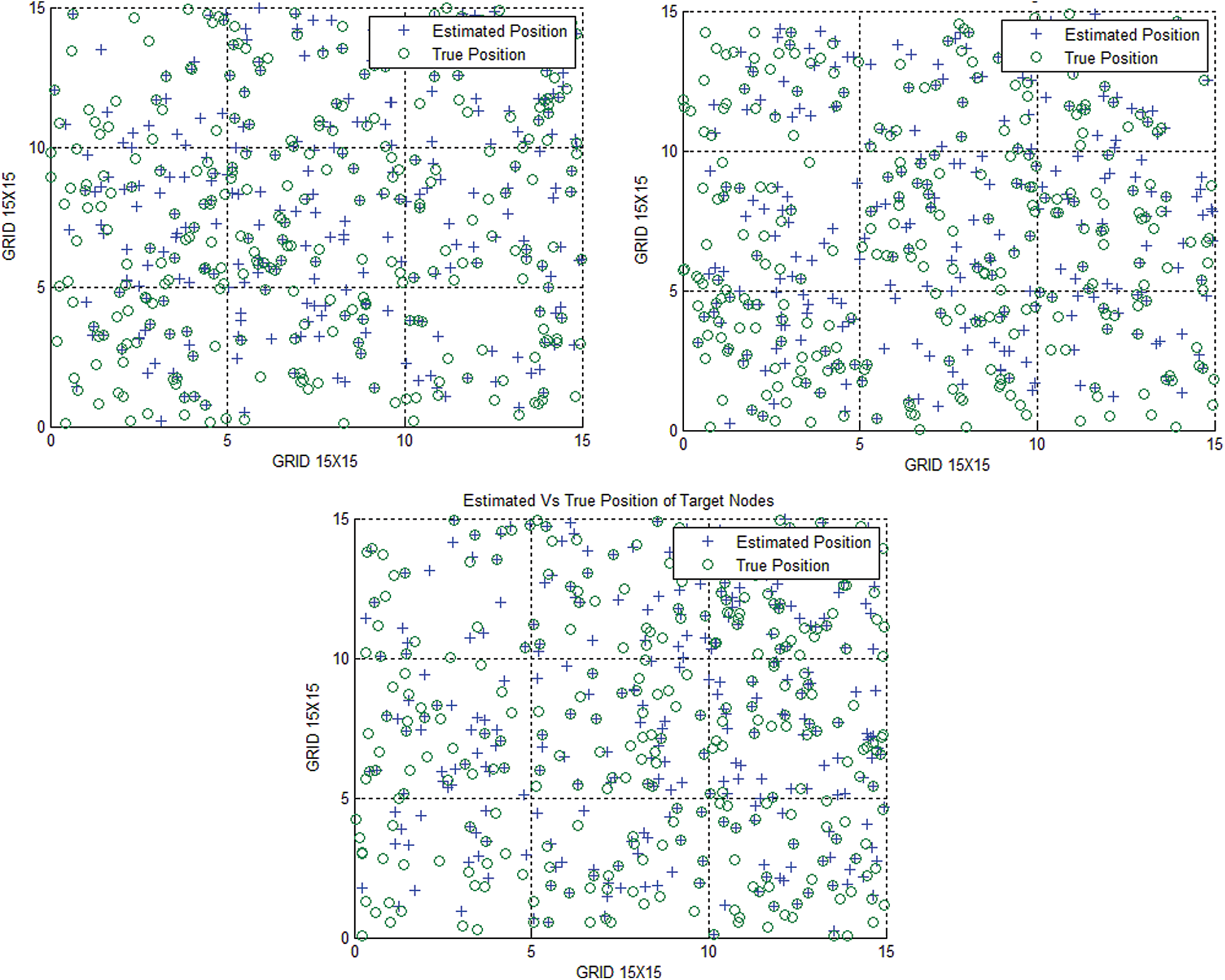
Figure 4: The different runs of proposed model

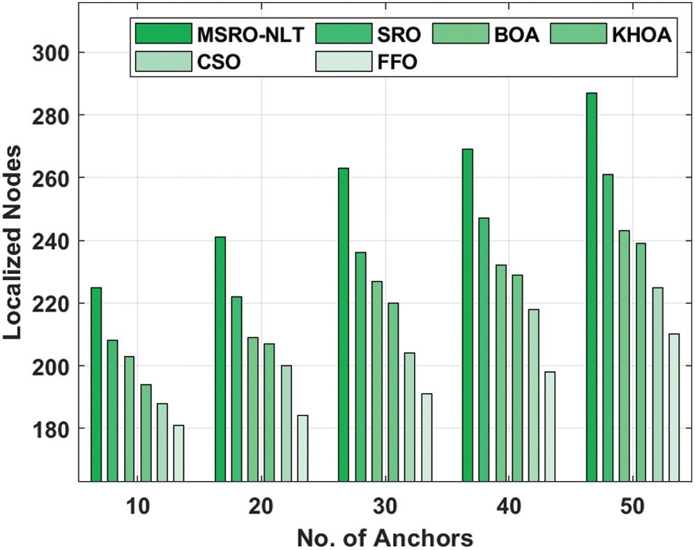
Figure 5: The NLN analysis of MSRO-NLT model

Meanwhile, on the existence of 30 anchor nodes, the MSRO-NLT approach has reached a maximum NLN of 263 whereas the SRO, BOA, KHOA, CSO, and FFO methodologies have attained a lesser NLN of 236, 227, 220, 204, and 191 correspondingly. At the same time, on the existence of 40 anchor nodes, the MSRO-NLT manner has achieved a maximum NLN of 269 whereas the SRO, BOA, KHOA, CSO, and FFO methods have achieved a minimal NLN of 247, 232, 229, 218, and 198 correspondingly. In line with that, on the existence of 50 anchor nodes, the MSRO-NLT approach has reached a higher NLN of 287 whereas the SRO, BOA, KHOA, CSO, and FFO techniques have obtained a lower NLN of 261, 243, 239, 225, and 210 correspondingly. A detailed localization error analysis of the MSRO-NLT technique with existing techniques takes place in Tab. 2 and Fig. 6.

The results portrayed that the MSRO-NLT technique has accomplished effective localization performance by obtaining a minimal localization error. For instance, with the presence of 10 anchor nodes, the MSRO-NLT technique has resulted a minimum localization error of 0.259 whereas the SRO, BOA, KHOA, CSO, and FFO algorithms have accomplished a maximum localization error of 0.4, 0.477, 0.585, 0.649, and 0.681 respectively. Moreover, with the presence of 20 anchor nodes, the MSRO-NLT model has resulted a minimal localization error of 0.197 whereas the SRO, BOA, KHOA, CSO, and FFO methods have accomplished a maximal localization error of 0.36, 0.427, 0.575, 0.629, and 0.672 correspondingly. Furthermore, with the presence of 30 anchor nodes, the MSRO-NLT manner has resulted a lesser localization error of 0.136 whereas the SRO, BOA, KHOA, CSO, and FFO approaches have accomplished a higher localization error of 0.340, 0.407, 0.485, 0.489, and 0.529 respectively. Along with that, with the presence of 40 anchor nodes, the MSRO-NLT method has resulted a lower localization error of 0.121 whereas the SRO, BOA, KHOA, CSO, and FFO techniques have accomplished a maximal localization error of 0.31, 0.357, 0.445, 0.529, and 0.493 correspondingly. At last, with the presence of 50 anchor nodes, the MSRO-NLT method has resulted a lesser localization error of 0.112 whereas the SRO, BOA, KHOA, CSO, and FFO methods have accomplished a maximum localization error of 0.26, 0.327, 0.455, 0.519, and 0.461 respectively. Tab. 3 and Fig. 7 examines the localization rate analysis of the MSRO-NLT technique with other existing methods under varying number of anchors.

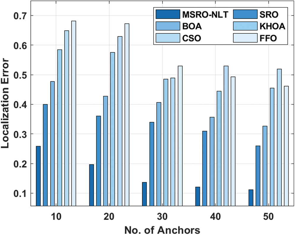
Figure 6: The result analysis of MSRO-NLT technique in terms of localization error

Tab. 4 and Fig. 8 investigates the localization error analysis of the MSRO-NLT technique under varying ranging error. The experimental values pointed out that the MSRO-NLT technique has obtained minimum localization error under different levels of ranging error. For instance, under the presence of 5% error, the MSRO-NLT technique has offered the least localization error of 0.256 whereas the SRO, BOA, KHOA, CSO, and FFO algorithms have demonstrated increased localization error of 0.390, 0.420, 0.600, 0.630, and 0.660 respectively. Meanwhile, under the presence of 10% error, the MSRO-NLT model has offered a minimum localization error of 0.221 whereas the SRO, BOA, KHOA, CSO, and FFO techniques have outperformed improved localization error of 0.360, 0.390, 0.580, 0.590, and 0.672 correspondingly. Eventually, under the presence of 15% error, the MSRO-NLT technique has offered a lesser localization error of 0.195 whereas the SRO, BOA, KHOA, CSO, and FFO approaches have showcased higher localization error of 0.340, 0.400, 0.460, 0.510, and 0.529 respectively. Simultaneously, under the presence of 20% error, the MSRO-NLT model has offered a minimal localization error of 0.132 whereas the SRO, BOA, KHOA, CSO, and FFO algorithms have exhibited superior localization error of 0.330, 0.340, 0.450, 0.450, and 0.493 respectively. Concurrently, under the presence of 25% error, the MSRO-NLT method has offered the least localization error of 0.117 whereas the SRO, BOA, KHOA, CSO, and FFO methodologies have portrayed maximum localization error of 0.300, 0.300, 0.400, 0.420, and 0.480 correspondingly.

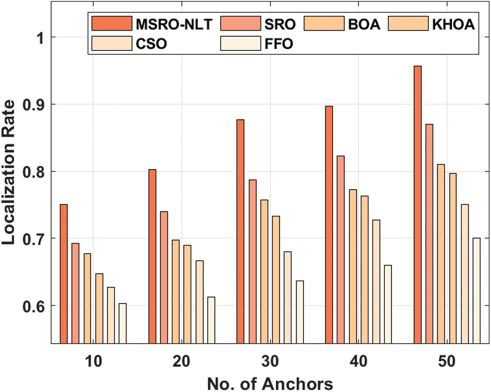
Figure 7: The localization rate analysis of MSRO-NLT technique

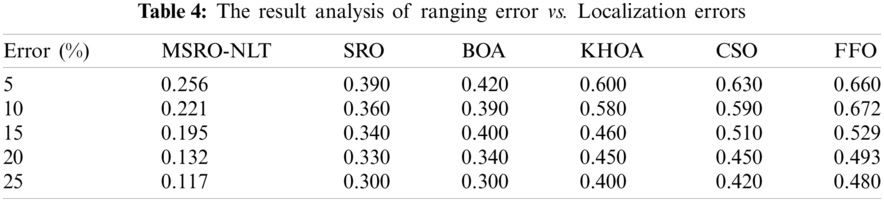
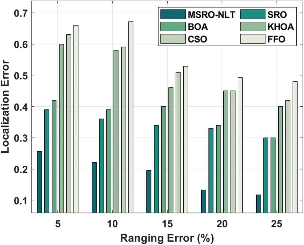
Figure 8: The localization error analysis of MSRO-NLT technique under distinct ranging error

From the above-mentioned tables and figures, it is evident that the proposed model is found to be an effective node localization technique over the compared methods.

5  Conclusion

This paper has presented a new MSRO-NLT technique for WSN. The MSRO-NLT technique aims to determine the exact locations of the unknown nodes that exist in the WSN. The MSRO algorithm inherits the concepts of SRO algorithm with the chaotic maps for improved diversity. The application of the concept of chaotic map to the characteristics of the traditional SRO algorithm helps to achieve better exploration ability of the MSRO algorithm. For assessing the proficient node localization results of the MSRO-NLT algorithm, a series of simulations were performed to showcase the improved localization performance of the MSRO-NLT technique. A comprehensive comparative results analysis showcased the betterment of the MSRO-NLT technique over the other compared methods in terms of different measures. As a part of future, hybrid metaheuristic algorithms can be designed for effective node localization in three-dimensional indoor environment.

Funding Statement: The authors received no specific funding for this study.

Conflicts of Interest: The authors declare that they have no conflicts of interest to report regarding the present study.

This work is licensed under a Creative Commons Attribution 4.0 International License, which permits unrestricted use, distribution, and reproduction in any medium, provided the original work is properly cited.