Computers, Materials & Continua DOI:10.32604/cmc.2022.018963
Article

Ambiguity Resolution in Direction of Arrival Estimation with Linear Antenna Arrays Using Differential Geometry

Alamgir Safi1, Muhammad Asghar Khan2,*, Fahad Algarni3, Muhammad Adnan Aziz1, M. Irfan Uddin4, Insaf Ullah2 and Tanweer Ahmad Cheema1

1Department of Electronic Engineering, ISRA University, Islamabad, 44000, Pakistan
2Hamdard Institute of Engineering & Technology, Islamabad, 44000, Pakistan
3College of Computing and Information Technology, University of Bisha, Bisha, Saudi Arabia
4Institute of Computing, Kohat University of Science and Technology, Kohat, Pakistan
*Corresponding Author: Muhammad Asghar Khan. Email: khayyam2302@gmail.com
Received: 28 March 2021; Accepted: 07 May 2021

Abstract: Linear antenna arrays (LAs) can be used to accurately predict the direction of arrival (DOAs) of various targets of interest in a given area. However, under certain conditions, LA suffers from the problem of ambiguities among the angles of targets, which may result in misinterpretation of such targets. In order to cope up with such ambiguities, various techniques have been proposed. Unfortunately, none of them fully resolved such a problem because of rank deficiency and high computational cost. We aimed to resolve such a problem by proposing an algorithm using differential geometry. The proposed algorithm uses a specially designed doublet antenna array, which is made up of two individual linear arrays. Two angle observation models, ambiguous observation model (AOM) and estimated observation model (EOM), are derived for each individual array. The ambiguous set of angles is contained in the AOM, which is obtained from the corresponding array elements using differential geometry. The EOM for each array, on the other hand, contains estimated angles of all sources impinging signals on each array, as calculated by a direction-finding algorithm such as the genetic algorithm. The algorithm then contrasts the EOM of each array with its AOM, selecting the output of that array whose EOM has the minimum correlation with its corresponding AOM. In comparison to existing techniques, the proposed algorithm improves estimation accuracy and has greater precision in antenna aperture selection, resulting in improved resolution capabilities and the potential to be used more widely in practical scenarios. The simulation results using MATLAB authenticates the effectiveness of the proposed algorithm.

Keywords: Antenna array; direction of arrival; ambiguity resolution; doublet antenna array; ambiguous observation model; estimated observation model

1  Introduction

Source localization through an array of sensors is always been a significant research direction in the past decades and even today and is widely utilized in various fields including radar, sonar, wireless communication and acoustics [1–4]. In this context, most commonly, uniform linear arrays (ULA) are used comprising of antennas usually spaced a half-wavelength apart. In order to achieve high resolution for more sources with the least number of antennas while keeping cost and hardware complexity low, linear arrays with antenna's spacing more than half-wavelength are deployed and numerous high-resolution algorithms like, Multiple Signal Classification (MUSIC) [5], JoDeG [6], Min-Norm [7], Space-Alternating Generalized Maximization-expectation (SAGE) [8] and Estimation of Signal parameters via Rotational Invariance Techniques (ESPRIT) [9], etc. have been proposed for one dimensional (1-D) direction of arrival (DOA) estimation problem.

Unfortunately, while increasing the spacing amongst the sensors of the linear antenna array from half-wavelength, although better resolution is achieved, under certain particular conditions, the array offers ambiguity among the angles of sources, and all these high-resolution algorithms generate an ambiguous error in the process of DOA estimation and the wrong estimation of DOA is achieved, which has a direct impact on the application of antenna array. This may result in misinterpretation of the target of interest [10]. For a linear array of antennas, an ambiguous error will occur, if any of the response vectors become a linear combination of two or more other response vectors. In such a case, this linear dependency amongst the response vectors leads to the failure of all these high-resolution algorithms in the identification of exact signal sources [11]. Briefly speaking, the larger the aperture of the array of sensors, the better the resolution achieved and more the array suffers from potential ambiguities [12].

The major problem in source localization with linear antenna array, having sensor spacing more than half-wavelengths is to resolve the directional ambiguity offered by the array due to its geometry. Aiming to resolve such a problem, we propose a novel algorithm based on the application of differential geometry. The proposed algorithm is based on a spatially designed doublet antenna array comprising of two different linear antenna arrays, having fixed sensor spacing, in terms of wavelength. Firstly, the corresponding responses of each individual antenna array are modeled using the concept of array manifolds. The shape of the manifold of a linear array of N omnidirectional antennas is a circular hyperhelix [13], located on an N-dimensional complex sphere. Due to such shape, application of differential geometry is much more convenient and beneficial in the analysis of geometrical properties of LA's and achieve dramatic results. Secondly, all possible an ambiguous set of directions exists in the manifold of each individual array are calculated based on uniform partitioning of their respective manifolds, and is obtained by dividing lengths of each manifold with their respective differences between any two sensor locations. For each antenna array, ambiguous set of directions calculated in this way is termed as an ambiguous observation model (AOM). The AOM calculated for both individual antenna arrays remain the same until the position of the sensors is fixed. Like AOM, each individual array has an angle observation model named as estimated observation model (EOM). The EOM for each individual array includes all the estimated angles via a direction-finding algorithm such as a genetic algorithm. The EOM calculated for both individual antenna arrays are off course not constant and gets updated when any source changes its position from its previous one. Finally, by utilizing both the observation models i.e., AOM and EOM for both individual arrays, the algorithm compares the EOM of each array with its corresponding AOM and selects the output of that array whose EOM has a minimum correlation with its corresponding AOM. Simulation results revealed that output selected in such a way is corrected and unambiguous.

Authors’ Motivation and Contribution

After a comprehensive literature review of the existing techniques for ambiguity resolution offered by a 1-D linear antenna array, it was observed that these techniques are based on hard problems and complex mathematics and hence, required high computational cost. These techniques suffer from rank deficiency issues and do not guarantee the required positive semidefinite augmented covariance matrix. Moreover, these techniques are constrained dependent and do not guarantee ambiguity resolution for generalized antenna array configuration. There is a critical need to propose a new generalized technique, which can successfully resolve the problem of ambiguity.

Motivated by the aforementioned objectives, the authors propose a new scheme for the resolution of ambiguities inherent in the manifold of a linear array. The proposed technique is based on differential geometry. Our contribution in this research work has some salient features as follows:

•   We introduce a novel architecture for designing a newly doublet antenna array, comprising of two independent linear arrays, whose sensor's positions are selected in such a way that, all ambiguous directions for both the arrays must be unique.

•   We propose an efficient technique along with genetic algorithm, which must choose unambiguous (true) direction of arrival of sources, impinging signals on the proposed doublet antenna array either from ambiguous or unambiguous directions using far field approximation.

•   The proposed technique when implemented along with the newly designed doublet antenna array, provides better and unambiguous results as compared to the classical method of ambiguity resolution using a single array.

•   The proposed algorithm improves estimation accuracy and has greater precision in antenna aperture selection, which predominantly improves the resolution capabilities of the antenna array.

The remaining paper is organized as follow: Section 2, presents related work on ambiguity resolution. Section 3, presents identification and calculation of all possible ambiguous sets and ambiguous generator sets for any linear array configuration. Section 4, introduces proposed technique along with its implementation and working to counter the problem of ambiguity inherent in the manifold of a linear array. Section 5, presents simulation results. Section 6, discusses performance comparison of DOA estimation using classical technique with the newly proposed technique, while Section 7, concludes the paper and suggest future work.

2  Related Work

2.1 Geometric Parameterization of Array Manifolds

The parameterization of different curves and surfaces can be obtained from a branch of mathematics known as differential geometry; see [13–15]. Differential geometry is the branch of mathematics which deals with the application of differential calculus to curves, surfaces and higher dimensional mathematical objects (manifolds) in order to investigate its geometrical properties.

Here are some basic concepts related to differential geometry which will we will be using in this article.

s=def∫0p⁡‖da_(p)dp‖dp(1)

dsdp=‖da_(p)dp‖(2)

s(θ)=π‖r_‖(1−cosθ)(3)

θ(s)=cos−1(1−sπ‖r_‖)(4)

2.2 Current Solutions

In this section, the authors explore related research on the ambiguity resolution problem. In reference [16] the authors proposed a generalized augmentation approach for fully augmentable array geometries, which successfully resolve manifold ambiguities for non-uniform linear arrays, with the approximation that the corresponding fisher information matrix must not be rank deficient [17]. However, it requires a high signal-to-noise ratio and a large number of snapshots, when there is minimum separation in terms of the spatial frequency amongst the ambiguous and unambiguous sources. Reference [18] presents, array interpolation method, to overcome the problem of rank deficiency. The technique presented can successfully recover the data from the elements of the virtual ULA's by imposing a linear interpolation on the elemental data of a real sparse linear array, and those coefficients are selected which has minimum interpolation error for a source impinging from a particular angular sector. However, disadvantage of using this technique is, it needs to know the angular sector. For improving the covariance matrix, the direct augmentation approach (DAA) is used in the proposed Toeplitz completion method [19], but unfortunately it does not guarantee the required positive semidefinite augmented covariance matrix. In order to construct such a matrix, an iterative DAA algorithm is proposed in [20,21], but unfortunately, it does not guarantee the global convergence due to its complicated iterative procedure. Wiener array interpolation is proposed in [22], which uses the maximum likelihood (ML) method to estimate SNR and utilize the calibration angles to recover the array steering matrix and can achieve the mean square error optimum solution. However, this method requires the initial DOA estimation. The proposed scheme in this research article differs from currents schemes, because it is quite simple, and is based on a doublet antenna array instead of a single antenna array. Due to the prior knowledge of the ambiguities for both individual arrays, calculated using differential geometry, the algorithm efficiently resolves the ambiguity problem.

3  Ambiguous Sets and Ambiguous Generator Sets

In this section, we are going to present the definition of Ambiguous set of DOA's and their rank of ambiguity.

Definition-1: Ambiguous Set: An order set of DOA's P_=[θ1,θ2,θ3,…,θm], is said to be an ambiguous set of DOA's

If m≤N and the matrix A(θ_)ϵCN∗m with columns the manifold vectors a_(θ1),a_(θ2),…,a_(θm) has rank < m i.e., rank(A(θ_))<m

Or

If m>N and all the subsets θ_i of θ_. which contains exactly N number of elements are themselves ambiguous set of DOA's i.e.,

Definition-2: Rank of Ambiguity: For any ambiguous set of DOA's rank of ambiguity is defined as;

In [23] the authors discussed issue related to rank-ambiguity of an array while estimating direction of arrival.

Definition-3: Ambiguous Generator set: If we have a set s_=[0,s1,s2,…,sc−1] comprising of “c” number of arc lengths where2≤c≤N. This set of arc lengths will be ambiguous generator set if all the following three conditions are satisfied.

i. First element of the set must be zero followed by the remaining non-zero elements.

ii. For the matrix, A(s_)ϵCN∗c rank of the matrix A(s_) should be less than c i.e., rank(A(s_))<c

iii. If we take any subset s_i consisting of “w” elements from the given set s_ with ρ≤w≤c then the rank(A(s_i))=ρ.

3.1 Identification of Ambiguous Generator Sets in Array Manifolds

This section presents identification and calculation of ambiguous generator sets (AGS) inherent in any linear array's manifold having arbitrary geometry by uniformly partitioning the Hyperhelices curve [11]. It should be noted here, that in [24] it has been proven that linear array having spatial array manifold are Hyperhelices curves. Hyperhelices curves are constant curvature curves. For a linear array, AGS is identified by partitioning the manifold into equal segments i.e.; uniform partitioning the manifold. This is achieved by dividing the manifold's total length lm through absolute difference between the locations of any two sensors of the same array (|ri−rj|) i.e., lm|ri−rj|.

The following theorem when applied to any linear array manifold will results in an ambiguous set.

Theorem 1: If we have a linear array consisting of N number of sensors in half wavelengths, with sensor's position r_=[r1,r2,…,rN]T then any subset consisting of N number of elements of the set of arc lengths s_i,jis an ambiguous set, if the following two conditions are true;

i)   Last element of the set of arc lengths s_i,j should be greater than zero and less than total length of the manifold (lm).

ii)   c≥N−1 where, c is number of non-zero elements.

Where,

s_i,j=[0,lm|ri−rj|,2lm|ri−rj|,3lm|ri−rj|,…,clm|ri−rj|]T∀i,j with i≠j(5)

clm|ri−rj|<lm⇒c={fix(||ri−rj||)if |ri−rj|∉N+|ri−rj|−1if |ri−rj|∈N+(6)

3.2 Calculation of Ambiguous Set of DOAs for Non-Uniform Linear Array

Steps for calculation of all possible ambiguous set of arc lengths and ambiguous set of directions inherent in the manifold of a non-uniform linear array are given below:

Step 1) Calculate the total length of the array manifold lm by using the formula lm=2π‖r_‖.

Step 2) Calculate Hadamard difference between sensor's positions with its self to get (N2×1) real vector i.e., Δr_=r_Θr_.

Step 3) Eliminate all entries of Δr_ which are lesser than unity to form a new vector Δr_˙. The idea of eliminating such entries is that it does not satisfy the first condition of Theorem 1. i.e., c=1+fix( Δrij) and cannot contribute in producing ambiguous generator sets.

where, Δr_˙∈Rd×1  and d=N2(N−1)

Step 4) Find out set of arc lengths s_i,j for each entry of the vector Δr_˙ by using Eq. (5). There will be total “d” set of arc lengths and each set of arc lengths corresponds to a different partition of the manifold.

Step 5) Identify those set of arc lengths s_i,j and get eliminated in which the number of nonzero entries is smaller than N−1. such entries should be eliminated because it cannot produce ambiguous generator sets.

Step 6) all the remaining set of arc lengths s_i,j must have same and equal lengths, if not then append zero where required.

Step 7) for each set of arc lengths, s_i,j calculate the AGS using the rules below.

Rule a) if all the nonzero elements of a set s_i,j are unique and do not repeat in any other set, then the number of ambiguous generator sets (AGS) produced by that particular set s_i,j are(cN−1). All these AGS's are possible subsets each having N number of elements of the same set s_i,j. All these ambiguous generator sets have rank of ambiguity=ρa=N−1.

Rule b) if all the nonzero elements of a set s_i,j are not unique and repeat in any other set then ambiguous generator sets having rank of ambiguity=ρa<N−1 might be achieved. All the subsets of that particular s_i,j with their first element 0 and with length 2,3,4,…,min(N,c+1) must be considered. For all these subsets to be ambiguous generator sets all the three conditions of definition-3 must be satisfied.

Step 8) Create a matrix M whose rows are the entire ambiguous generator sets found in Step 7. Eliminate the duplicate rows if any.

Step 9) for the matrix Mabove,calculate matrix θAmbig using Eq. (4) which consist of all the ambiguous set of directions in terms of degrees.

4  Proposed Technique and Its Implementation

In this study, we aim to resolve the problem of ambiguity offered by any linear antenna array configuration in the process of direction of arrival estimation of sources. For this purpose, we propose a new technique which gives unambiguous results irrespective of the impinging signals. Unlike the classical method of DOA estimation, which uses a single antenna array, the proposed technique is based on a newly designed doublet antenna array.

4.1 Designing of the Doublet Antenna Array

We aim to design a new array in such a way that it includes two different linear arrays i.e., array 1 and array 2, both having different sensor positions, which makes it a doublet antenna array. r_1 is the vector which represents the location of sensors for array 1 (A1) and r_2 is the vector which represent the location of sensors for array 2(A2). In order to make the overall output of proposed array ambiguity free, we must choose r_1andr_2 i.e., antenna's separation for both the individual arrays carefully, so that the ambiguous set of arc lengths and hence ambiguous set of directions for both the arrays are unique i.e., no ambiguities should be common among both the arrays or the two sets of ambiguities should be completely disjoint. Fig. 1 represents the proposed architecture for designing an ambiguity-free antenna array.

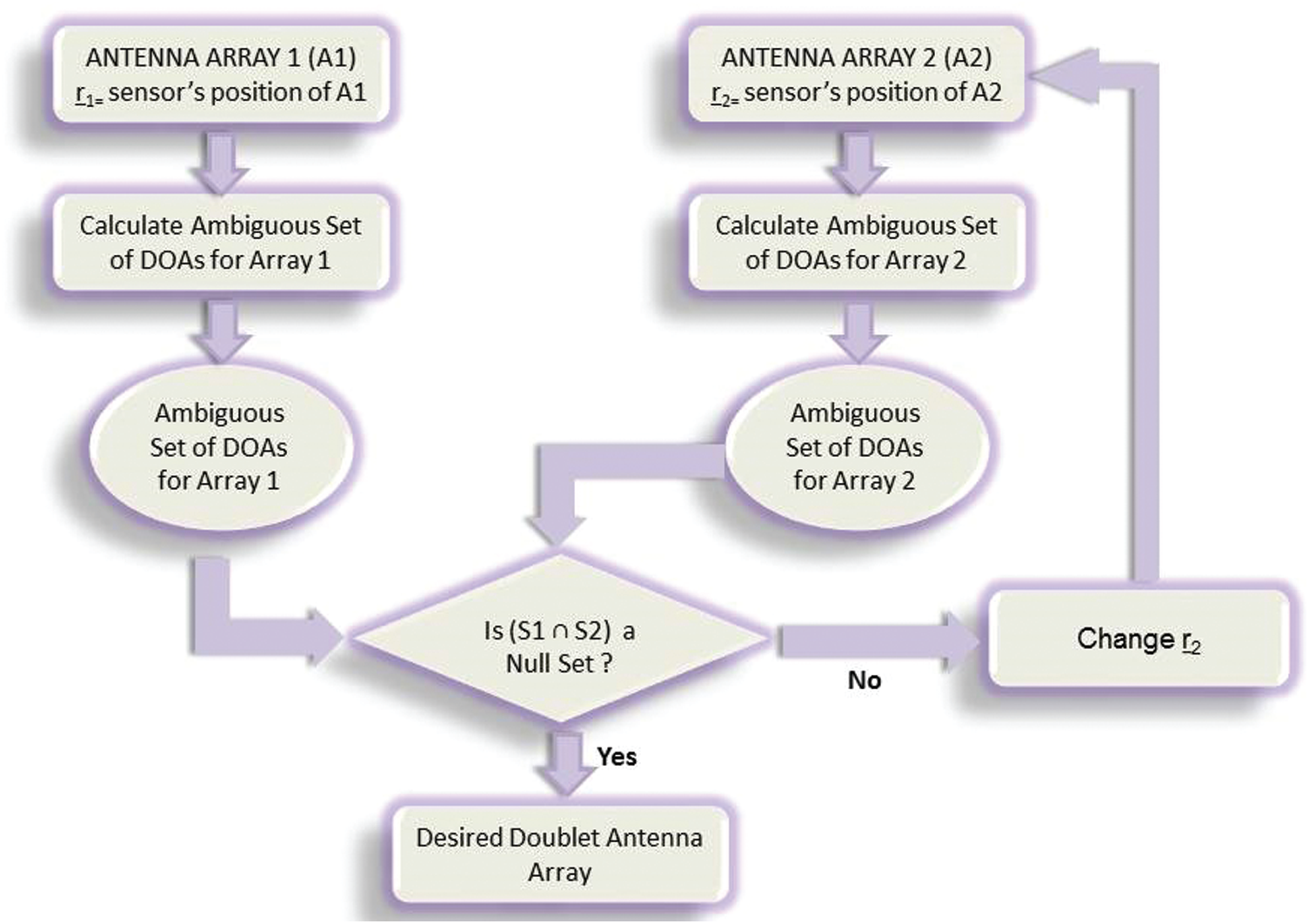
Figure 1: Architecture for our proposed doublet antenna array

In order to achieve the desired doublet antenna array in which both the individual antenna array must not have any ambiguous angles common, then we have to choose the position of the antenna elements for both the arrays i.e., r_1 and r_2 in such a way that there should be no inter-sensor spacing common in between both the arrays. In light of the proposed architecture for designing a doublet antenna array, we choose, r_1=[−3 −1 −0.52 2.5] and r_2=[−3.5 −0.25 3.75 5.1] wherer_1andr_2are the vectors which represents the location of sensors in half wavelengths for array 1 and array 2 respectively. The ambiguous sets of directions i.e., ambiguous observation model (AOM) for both the arrays are calculated below:

● Calculations of AOM for Array 1:

a) a. Manifold's length = lm=28.4483

b) b. Hadamard difference between vector representing sensor's positions with its self after eliminating those entries which are smaller than unity is Δ_r1 i.e.,

c) c. Dimension of Δ_r1 is d=8, so eight uniform basic sets exist and are listed in Tab. 1

d) d. That uniform basic set which has less than N−1 non-zero elements are eliminated. We can clearly see from Tab. 1 that only the set sΔr1,4T and sΔr1,5T satisfies the second condition of Theorem 1 i.e., c≥N−1 Where c is number of non-zero elements and hence, both of them are the ambiguous set of arc lengths.

e) e. Make the length of both set of arc lengths equal since length of sΔr1,5T and sΔr1,4T are not equal. So Matrix S consisting of set of ambiguous arc lengths is

f) f. Ambiguous generator sets (AGS) is calculated for both set of arc lengths using rule 7(a) as both these set are unique and do not repeat. AGS produced by each set of arc lengths are (cN−1).

For row1{S}: c=4 and N=5 so(44)=1 ambiguous generator set is produced Row1{S} i.e.,

For row2{S}: c=5 and N=5 so, (54)=5 ambiguous generator sets is produced by Row2{S} by taking all the subsets of N elements of Row2{S} i.e.,

g. Create Matrix M whose rows are all the Ambiguous generator sets produced above i.e.,

h. Ambiguous set of directions for all the elements of M in terms of degrees are calculated using Eq. (4). All the ambiguous DOA's (In Degrees) can be written in matrix form as,

•   Calculation of AOM for Array 2:

Manifold's length = lm=45.4761

Hadamard difference between vector representing sensor's positions with its self after eliminating those entries which are smaller than unity is Δ_r2 i.e.,

Dimension of Δ_r2 is d=6, so there are six uniform basic sets exists and are listed in Tab. 2.

That uniform basic set which has less than P−1 non-zero elements are eliminated. We can clearly see from Tab. 2 that only the set sΔr3,4T does not satisfy the second condition of Theorem 1 i.e., c≥P−1 Where c is number of non-zero elements and hence eliminated.

Make the length of all set of arc lengths equal if not. So Matrix S consisting of set of ambiguous arc lengths all with equal lengths.

Ambiguous generator sets (AGS) is calculated for all set of arc lengths using rule 7(a) as all these sets are unique and do not repeat. AGS produced by each set of arc lengths are (cP−1). Here for simplicity we are not showing the ambiguous generator sets due to large number of sets.

For row1{S}: c=3 and P=4 so(33)=1 ambiguous generator set is produced Row1{S} i.e.,

For row2{S}: c=7 and N=P so, (73)=35 ambiguous generator sets is produced by Row2{S} by taking all the subsets of P elements of Row2{S}.

For row3{S}: c=8 and P=4 so, (83)=56 ambiguous generator sets is produced by Row3{S} by taking all the subsets of P elements of Row3{S}.

For row4{S}: c=3 and P=4 so, (33)=1 ambiguous generator sets is produced by Row4{S} by taking all the subsets of P elements of Row4{S}.

For row5{S}: c=5 and P=4 so, (53)=10 ambiguous generator sets is produced by Row2{S} by taking all the subsets of P elements of Row5{S}.

g.   Matrix M contains all the ambiguous generator sets produced above. For simplicity we are just showing the ambiguous generator sets produced for Row5{S}.

h.   For simplicity we are stating only few of the ambiguous set(s) of directions for array 2 i.e., θAmbig(Array2)

It should be noted that all the values containing both θAmbig(Array1) and θAmbig(Array2) are in degrees. From θAmbig(Array1) and θAmbig(Array2) we can clearly see that both the arrays have different sets of ambiguous directions because we have chosen r_1andr_2 in such a way that none of the inter-sensor spacing between both the arrays is common. In this case our proposed technique will work accurately and the overall output of the doublet array is unambiguous. i.e., Our direction finding algorithm works efficiently. But if we deliberately choose r_1andr_2 in a way that there are common inter-sensor spacing's between the arrays, than in that case, common ambiguous directions exists and the algorithm does not work effectively, and the overall output of the proposed doublet antenna array might become ambiguous.

4.2 Proposed Technique and It's Working

In Section 4.1, we have designed a doublet antenna array in such a way that no ambiguous directions are common among both the individual arrays. Also for each of the individual antenna array ambiguous set of DOA have been calculated. Fig. 2 represents signals impinging on the doublet antenna array from a single source, assuming far field approximation.

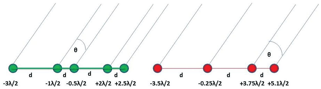
Figure 2: Signals impinging on designed doublet antenna array from far field

Green filled circles represent position of antenna's for array 1 in terms of half wavelengths, while red filled circles represent antenna's position of array 2 in terms of half wavelength. The position of all the antennas are selected according to Fig. 1. Genetic Algorithm (GA) is used as a direction finding (DF) algorithm for estimation of DOA of signals impinging on the designed doublet array shown in Fig. 2 and has been implemented in Matlab R2014b as a simulation tool, assuming five (05) sources.

Fig. 3 represents a flow chart which shows working of GA. Due its heuristic and globally convergence nature it works quite well in DOA estimation, and provide best possible directions of all the sources impinging on antenna array. Fig. 4 illustrates working of the proposed technique along with genetic algorithm, which chooses unambiguous (true) DOA of different sources impinging on designed array using far field approximation. After the sources imping signals from far field on the doublet antenna array, all possible ambiguous sets of DOA i.e., ambiguous observation model are calculated for both arrays. After that genetic algorithm estimates DOA of all the sources simultaneously for both the arrays i.e., estimated observation model is calculated. Once the EOM of all the sources for both arrays is achieved; the proposed technique compares all the estimated DOA of sources for both the individual arrays with all the ambiguous sets of DOA. If all the estimated DOA of sources does not belong to any of the ambiguous sets of DOA, then there is no ambiguity exists in the estimated DOAs of both the arrays i.e., DOA estimation of both the arrays are correct and the algorithm chooses either output of array 1 or array 2. But if the estimated DOA by any of the array belongs to any ambiguous set of DOA, then the problem of ambiguity is said to arise, and in such case the algorithm will have to decide the unambiguous/correct DOA as follow:

a. If the estimated DOA either by array 1 or array 2 belongs to any ambiguous sets (or subset) of array 1, then choose output of array 2. In other words, output of that array should be selected which gives a null set when taking intersection with their own ambiguous sets.

b. If the estimated DOA either by array 1 or array 2 belongs to any ambiguous sets (or subset) of array 2, then choose output of array 1. In other words, output of that array should be selected which gives a null set when taking intersection with their own ambiguous sets.

c. If the estimated DOA either by array 1 or array 2 belongs to both ambiguous sets of array 1 and array 2, then choose output of that array is selected whose EOM has minimum correlation with its AOM. It is important to be noted here that in our proposed technique, the comparison is done by flooring down both the value i.e., both the estimated and ambiguous DOAs. This could be done because genetic algorithm is a heuristic technique which not necessarily estimates the exact fractional values of a decimal number.

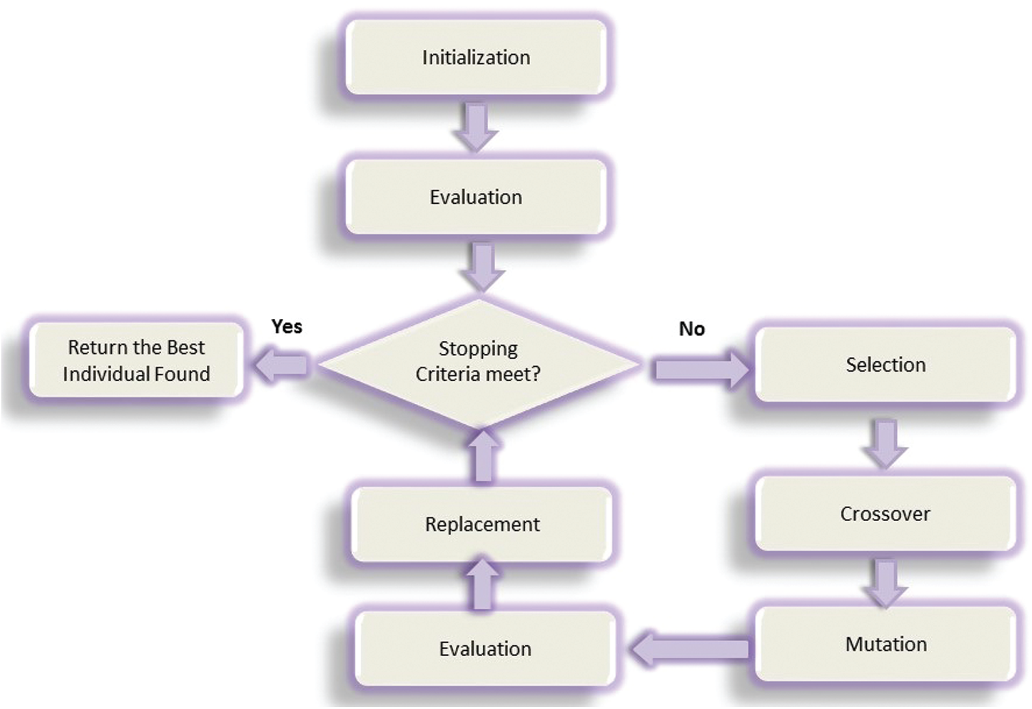
Figure 3: Working of genetic algorithm (GA)

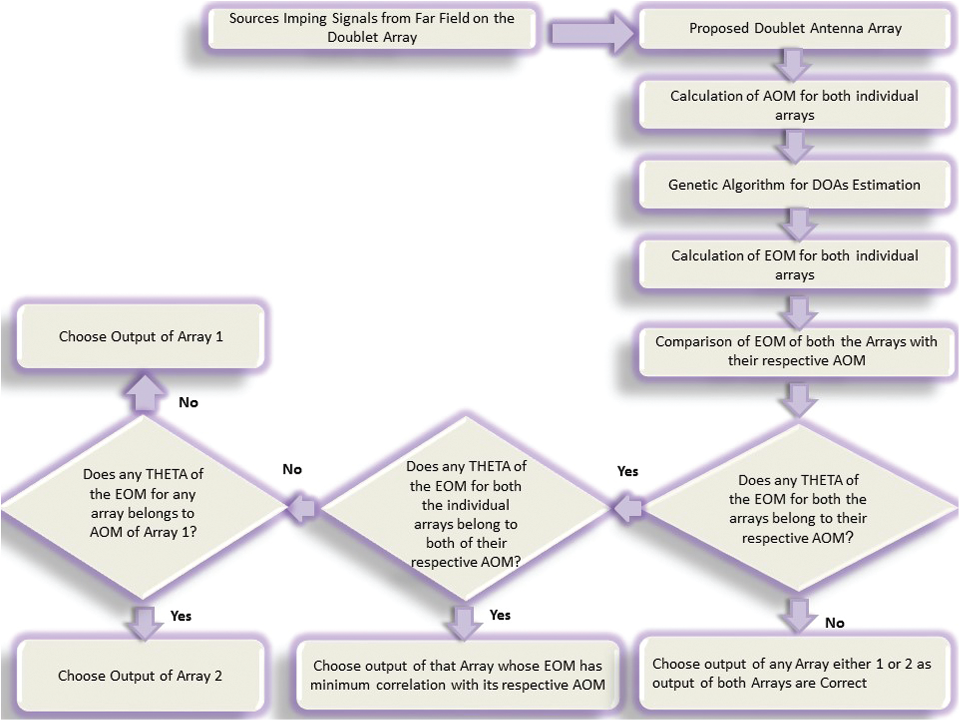
Figure 4: Working of the proposed algorithm, which choose unambiguous (true) direction of sources, which impinge signals on the proposed doublet antenna array. Output of that array is selected, whose EOM has minimum correlation with its corresponding AOM

5  Results

The proposed doublet antenna array is used for DOA estimation of 5 sources, along with direction finding algorithm i.e., GA implemented in Matlab R2014b. For the proposed doublet array, simulations have been carried out in three different scenarios i.e., all sources impinging signals on the doublet array from ambiguous, unambiguous and semi ambiguous directions and the results are tabulated in Tab. 5. In order to compare results of the proposed technique with the classical technique of DOA estimation i.e., DOA estimation using a single array, simulations for both the techniques (proposed technique and classical technique) are performed. Tabs. 3 and 4 shows simulation results in case of a using a single array i.e., array 1 and array 2 respectively.

•   GA Parameters are:

No. of sources = 5, No. of cycles = 2000, Error threshold = 0.001.

Number of required chromosomes = 400, Number of genes in each chromosome = 10.

•   Cost function = ‖‖Ynorm(Y)⋅YHATnorm(YHAT)‖−1‖ where, Y is the received observations at the doublet array input and YHAT is the estimated observations by GA.

5.1 Direction of Arrival Estimation Using Classical Technique

In classical method of DOA estimation, when using a single array for DOA estimation, i.e., array 1, then, if signals impinging on the array are from ambiguous direction(s) (from any of the ambiguous set of DOAs calculated for array 1) then the output is wrong/ambiguous. In case, if the signals impinging on array 1 from unambiguous directions (does not belong to any of the ambiguous set of DOAs calculated for array 1) then the response of the array is correct/unambiguous. Simulations are performed for array 1 to show its behavior to the signals impinging either from ambiguous or unambiguous directions. Results are tabulated in Tab. 3. Similar is true for array 2 whose results are presented in Tab. 4.

•   Simulation Results for Array 1

For array 1 i.e., r_1=[−3 −1 −0.5 2 2.5] where r_1 represents sensor's position for array 1.

i)   Case 1: All signals impinging on array 1 are from ambiguous directions i.e., THETA = [0 53.1301 78.4630 101.5370 126.8699]. In this case Genetic Algorithm is not accurately estimating directions of all the signals impinging on array 1. Instead of estimating 101.5370∘ for the fourth source, GA estimates 95.3149∘ which is almost an ambiguous direction for the same array. Moreover, due to ambiguity offered by the array to the given set of DOA's, GA is incapable of accurately estimating other directions as well. Estimated DOA's are listed in Tab. 3.

ii)   Case 2: All signals impinging on array 1 are from another set of ambiguous directions i.e., THETA = [0 50.4788 74.1734 117.0357 144.9032]. In this case GA is not accurately estimating directions of all the signals impinging on array 1. Instead of estimating 50.4788∘ for the second source, Genetic Algorithm estimates 53.2108∘ which is almost an ambiguous direction for the same array. Estimated DOA's are listed in Tab. 3.

iii)   Case 3: All signals impinging on array 1 are from unambiguous directions i.e., THETA = [0 39.8753 57.6640 72.4027 85.9994]. In this case GA is accurately estimating direction of all the sources which impinge signals on array 1. Estimated DOA's are listed in Tab. 3.

•   Simulation Results for Array 2

For array 2 i.e., r_2=[−3.5 −0.25 3.75 5.1] where r_2 represents sensor's position for array 2.

i)   Case 1: All signals impinging on array 2 are from ambiguous directions i.e., THETA = [0 39.8753 57.6640 72.4027 85.9994]. In this case GA is not accurately estimating directions of all the signals impinging on array 2. Instead of estimating 72.4027∘ for the fourth source, Genetic Algorithm estimates 63.3785∘ which is almost an ambiguous direction for the same array. Moreover, due to ambiguity offered by the array to the given set of DOA's, GA is incapable of accurately estimating other directions as well. Estimated DOA's are listed in Tab. 4.

ii)   Case 2: All signals impinging on array 2 are from ambiguous directions i.e., THETA = [0 43.6028 63.3669 80.0718 130.9327]. In this case GA is not accurately estimating directions of all the signals impinging on array 2. Instead of estimating 80.0718∘ for the fourth source, Genetic Algorithm estimates 85.6576∘ which is almost an ambiguous direction for the same array. Estimated DOA's are listed in Tab. 4.

iii)   Case 3: All signals impinging on array 2 are from unambiguous directions i.e., THETA = [0 53.1301 78.4630 101.5370 126.8699]. In this case GA accurately estimates direction of all the sources which impinge signals on array 2. Estimated DOA's are listed in Tab. 4.

5.2 Direction of Arrival Estimation Using the Proposed Doublet Antenna Array

Simulations are performed for the following five (05) cases using our proposed doublet array and results are tabulated in Tab. 5.

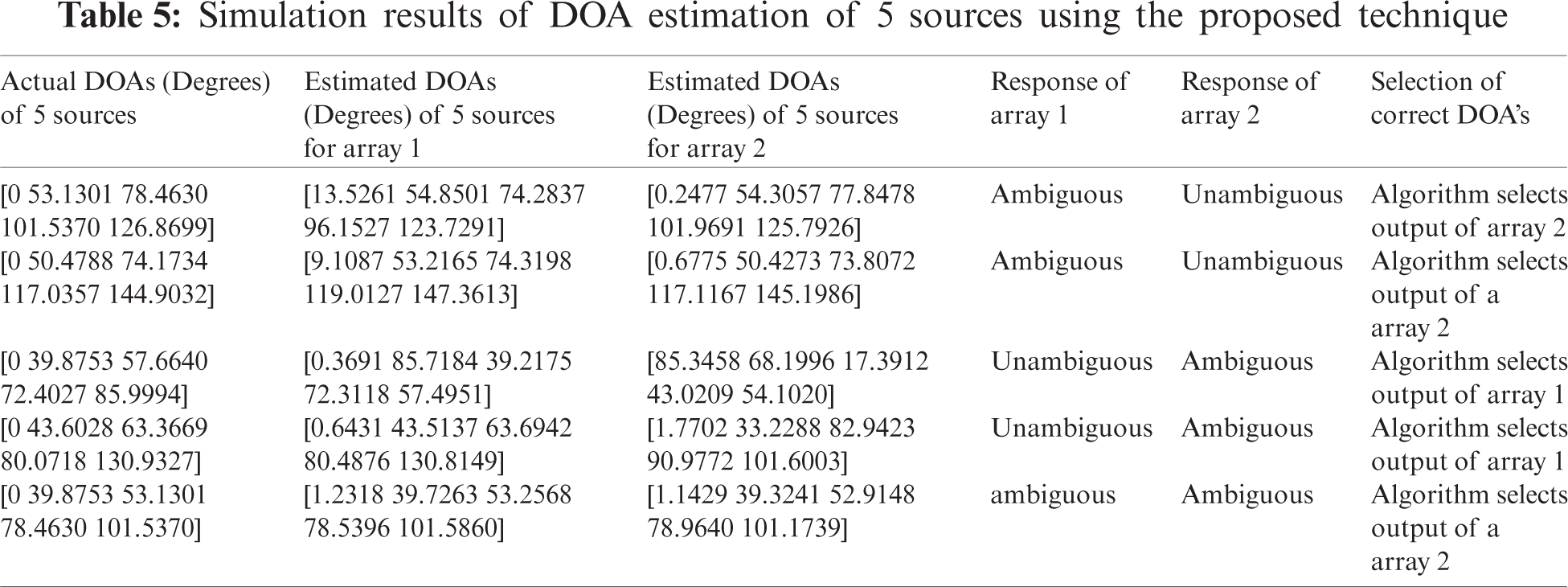
i)   Case 1: THETA = [0 53.1301 78.4630 101.5370 126.8699] i.e., All these DOA's are unambiguous for array 2 but ambiguous for array 1 because all of them belong to θAmbig(Array1). In this case Genetic Algorithm is accurately estimating directions of all the signals impinging on array 2 while the directions estimated for array 1 are ambiguous because EOM when compared with the AOM does not give a null set, which means that one or more of the directions are ambiguous, so the proposed algorithm selects output of array 2. Results are tabulated in Tab. 5.

ii)   Case 2: THETA = [0 50.4788 74.1734 117.0357 144.9032] i.e., All these DOA's are unambiguous for array 2 but ambiguous for array 1, because all of them belong to θAmbig(Array1). So the proposed algorithm selects output of array 2. Results are tabulated in Tab. 5.

iii)   Case 3: THETA = [0 39.8753 57.6640 72.4027 85.9994] i.e., All these DOA's are unambiguous for array 1 but ambiguous for array 2, because all of them belong to θAmbig(Array2). So the proposed algorithm selects output of array 1. Results are tabulated in Tab. 5.

iv)   Case 4: THETA = [0 43.6028 63.3669 80.0718 130.9327] i.e., All these DOA's are unambiguous for array 1 but ambiguous for array 2, because all of them belong to  θAmbig(Array2). So the proposed algorithm selects output of array 1. Results are tabulated in Tab. 5.

v)   Case 5: THETA = [0 39.8753 53.1301 78.4630 101.5370] i.e., All these DOA's are partially ambiguous for both arrays because all of them belong to θAmbig(Array1) and θAmbig(Array2). In such circumstances, the algorithm selects output of that array, whose EOM has minimum correlation with its corresponding AOM. In this case the algorithm selects output of array 2 because, the output of array 2 has only a single estimated DOA that is matched with their ambiguous DOA i.e., estimated DOA for array 2 is 39.3241∘ while the ambiguous DOA is 39.7263∘. It should be noted that all the values should be floor down before correlation. Results are tabulated in Tab. 5.

6  Performance Comparison

After carried out simulations for DOA estimation using the classical technique, as well as, utilizing our proposed technique for different cases, we observed that the proposed technique estimates all the DOAs impinging on the doublet antenna array accurately without giving any overall ambiguous results. From Tab. 5, we can see that almost all the impinging signals from different directions were somehow ambiguous for the doublet array either for array 1 or array 2, but the results achieved using the proposed technique are correct/unambiguous. If we compare the results achieved with the proposed technique given in Tab. 5 with the results achieved using a classical technique of DOA estimation given in Tabs. 3 and 4, we can see that the results achieved with a classical technique faces the problem of ambiguity in case if, the impinging signals on the array are from ambiguous directions. While in the case of DOA estimation using the proposed technique, we always achieve correct/unambiguous results irrespective of the direction of the impinging signals. So the proposed technique works well, although the impinging signals on the doublet array are from ambiguous directions, whereas, the classical technique fails under such scenarios.

7  Conclusions and Future Work

In this research article, we proposed a newly designed doublet antenna array along with an efficient technique for estimation of direction of sources by utilizing the concept of differential geometry and its application in antenna array processing. GA is used to estimate the directions of sources without having any ambiguity. The proposed technique was shown to be efficient against the ambiguous directions of sources, as compared to the classical methods for direction estimation using a single array. We have seen that the application of differential geometry in antenna array processing for the identification of ambiguities in a linear array, provides good grounds for resolving the ambiguities inherent in the manifold of a non-uniform linear array. In the future, we intend to propose a technique for resolving the problem of ambiguities inherent in the manifolds of planer arrays with the application of differential geometry.

Acknowledgement: The authors would like to thank the reviewers for their time and review.

Availability of Data and Materials: The data used for the findings of this study is available upon request from the corresponding authors.

Funding Statement: The authors received no specific funding for this study.

Conflicts of Interest: The authors declare that they have no conflicts of interest to report regarding the present study.

This work is licensed under a Creative Commons Attribution 4.0 International License, which permits unrestricted use, distribution, and reproduction in any medium, provided the original work is properly cited.