Computers, Materials & Continua DOI:10.32604/cmc.2022.018735
Article

Attention-Based and Time Series Models for Short-Term Forecasting of COVID-19 Spread

Jurgita Markevičiūtė1,*, Jolita Bernatavičienė2, Rūta Levulienė1, Viktor Medvedev2, Povilas Treigys2 and Julius Venskus2

1Institute of Applied Mathematics, Vilnius University, Vilnius, 03225, Lithuania
2Institute of Data Science and Digital Technologies, Vilnius University, Vilnius, 08412, Lithuania
*Corresponding Author: Jurgita Markevičiūtė. Email: jurgita.markeviciute@mif.vu.lt
Received: 19 March 2021; Accepted: 02 May 2021

Abstract: The growing number of COVID-19 cases puts pressure on healthcare services and public institutions worldwide. The pandemic has brought much uncertainty to the global economy and the situation in general. Forecasting methods and modeling techniques are important tools for governments to manage critical situations caused by pandemics, which have negative impact on public health. The main purpose of this study is to obtain short-term forecasts of disease epidemiology that could be useful for policymakers and public institutions to make necessary short-term decisions. To evaluate the effectiveness of the proposed attention-based method combining certain data mining algorithms and the classical ARIMA model for short-term forecasts, data on the spread of the COVID-19 virus in Lithuania is used, the forecasts of epidemic dynamics were examined, and the results were presented in the study. Nevertheless, the approach presented might be applied to any country and other pandemic situations. The COVID-19 outbreak started at different times in different countries, hence some countries have a longer history of the disease with more historical data than others. The paper proposes a novel approach to data registration and machine learning-based analysis using data from attention-based countries for forecast validation to predict trends of the spread of COVID-19 and assess risks.

Keywords: COVID-19 spread modeling; attention-based forecasting; machine learning; data registration; data analysis; ARIMA

1  Introduction

The COVID-19 pandemic has added an extremely high element of unpredictability to the global economy and the situation in general. Governments are trying to overcome the infection by taking serious measures in an effort to stabilize the situation. Experts are trying to predict how the situation may change and how it will look when the coronavirus can be restrained and which states will be the first to come out of the economic recession. At the moment, the priority is to solve urgent health care problems and maintain economic stability. Experts are already trying to look into the near future and understand how the disease rate can progress.

Short-term and long-term forecasting models are generally used to forecast certain situations and to alert us to events in the future so that we are better prepared. Short-term forecasting models [1], which predict for no more than a few days, react and reflect more up-to-date data than long-term models. The latest new data in long-term models has a much less impact on the forecast growth curves as the more recent data form a much smaller proportion of the total. Therefore, to create accurate short-term forecasts, it is necessary to be especially careful and pay attention to the up-to-date data on new cases. Practice shows that stochastic methods are most effective for short-term forecasts, while deterministic methods, like SIR or SEIR [2,3], are most suitable for describing long-term scenarios.

Effective short-term prediction models are needed to predict the number of new cases. In this regard, it is important to develop strategic planning methods in the public health care system to avoid further increases in incidence of infection, as well as to introduce special measures to reduce the scope of infection. Various methods based on mathematical modeling and data mining are powerful tools for understanding the COVID-19 transmission [4], as well as for modeling and studying different scenarios for short-term pandemic forecasting. The accuracy of forecasting methods largely depends on the quality and quantity of available data used to make forecasts and assess the situation. The problems of forecasting the dynamics of confirmed cases of COVID-19 are being widely discussed in many recent scientific publications [5–13].

Despite the limitations associated with medical data-based forecasting and the specific nature of the data being analyzed, forecasting plays an important role as it enables a better understanding of the current situation and makes plans for the future. Mathematical modeling and disease prediction are powerful tools for understanding the spread of COVID-19 and studying different scenarios. Various methods and time series analysis are currently being used for short-term forecasting of COVID-19 epidemic disease dynamics: linear forecasting models, including autoregressive integrated moving average (ARIMA) model [5,14–16], artificial intelligence inspired models [10,13,17–19], hybrid forecasting models [20–22]. Because of the limited amount of data available, models inspired by artificial intelligence were not used in this study. The authors propose an attention-based method and compare short-term forecasting results with the simple but effective ARIMA model for forecasting disease spread trends. By means of machine learning clustering, the authors of this paper draw attention to countries with a longer COVID-19 disease spread history and, based on the data obtained, calculates the forecast for the country under study. According to the recent research [5], two criteria are emphasized: the accuracy of forecasts and the simplicity of the models used. A variety of applicable strategies make it possible to combine several methods, such as data preprocessing, data mining methods, and common forecasting models. ARIMA model has the advantage of a simple structure and a strong ability to interpret the data. Rather than focusing on which model is more correct, we need more models that answer additional questions and the use of which may affect the spread of COVID-19 [23].

The main purpose of this article is to provide short-term forecasting that could produce a reliable forecast for policymakers to make the necessary decisions and to provide useful guidance. In this paper, the authors provide the results of statistical forecasting of confirmed cases of COVID-19 in Lithuania using the attention-based approach and ARIMA models. The proposed methods might be applied to any country and other pandemic situations. The paper is organized as follows: Section 2 presents the analyzed data and methodology for short-term forecasting of confirmed cases of COVID-19 using the ARIMA models and the attention-based machine learning method. The experimental results of the proposed method as well as the comparison with Lithuanian forecasting results obtained using the ARIMA models are presented in Section 3. The results of the study are concluded in Section 4.

2  Materials and Methods

2.1 Data in the Context of Lithuania

During the pandemic, the source of Lithuanian COVID-19 data changed, which made the task of spread forecasting challenging. The main data provider in Lithuania is the National Public Health Center (NPHC) under the Ministry of Health. Since the beginning of the spread of COVID-19 in Lithuania, the data has been announced on the website of the Ministry of Health. The problem with such an announcement was that no historical data was available, only the daily statistics, thus the authors had to collect, process, and store data by creating their own database. However, because of problems with data collection in the NPHC–delays by various institutions, errors caused by human factors, etc.–historical data has also been revised, but this has not been announced. At first, the revisions were not substantial and did not affect the short-term forecasts. However, corrections became substantial before the autumn of 2020, when the number of confirmed cases increased. Since the end of August, the National Public Health Center under the Ministry of Health started sharing files with the time series data. Although there were still problems with the quality of the data, but historical data became available. Since November, the only institution announcing the COVID-19 data is Statistics Lithuania.1 Although the quality problems have not been completely resolved, detailed daily datasets with revised historical data are now available.

Nevertheless, it has been noticed that some time series, such as recoveries or active cases, still suffer from quality problems due to delays in reporting recoveries by hospitals. Thus, in the middle of February 2021, Statistics Lithuania started announcing two time series for recovered and active cases: a de jure series, which announces registered cases and statistical series, which announces statistical estimates. These time series are very different from each other and have differences with the earlier recovered and active cases time series.

The authors use data2 from the Coronavirus Resource Centre (CRC) at Johns Hopkins University as a data source for other countries. It was noticed that Lithuanian historical data of the disease was not correctly updated in the CRC source. Thus, while analyzing Lithuania in the context of the European countries, the authors used the data from Lithuanian data sources rather than from the CRC. For the clustering and attention-based forecasting, European countries and COVID-19 data of confirmed, recovered cases, deaths from COVID-19 per 100,000 people, and population density from the United Nations database on 2019 mid-year period was used in the research. The motivation for including population density was based on the assumption that more densely populated countries have a higher risk of more rapid spread of COVID-19.

Despite the fact that the beginning of confirmed cases of COVID-19 in Lithuania is February 28, 2020, the authors in this research use data on the spread of the disease in Lithuania during the period from March 12, 2020, to February 1, 2021, because only one case was registered until March 12, 2020. Moreover, we take the earlier definition of recovered cases since new definitions have appeared after the period we are investigating. Fig. 1 shows the dynamics of the daily confirmed cases and cumulative confirmed cases per 100,000 people. There was a huge increase in the number of confirmed cases per day in the autumn of 2020 and January 2021, while the spring and summer of 2020 were relatively stable periods. There are several reasons for this. In spring 2020, Lithuania announced a very strict lockdown–schools, kindergartens, and universities switched to online learning, all non-food shops and services were closed, only online trade was allowed, the number of imported cases was higher than inside the country; thus, the closure of borders helped to reduce the spread of COVID-19. During the summer period, a small number of confirmed cases might be possibly related to the reduced extent of traveling abroad and weather conditions. During the autumn there was no strict lockdown, mostly recommendations, schools and kindergartens operate in normal or mixed mode, universities operate in online or mixed mode. Thus, the spread becomes very intensive, and the prevention becomes belated and unresponsive to the actual situation of COVID-19. Therefore, as most cases occur within the country, border closures are not used to prevent the spread of the COVID-19 virus.

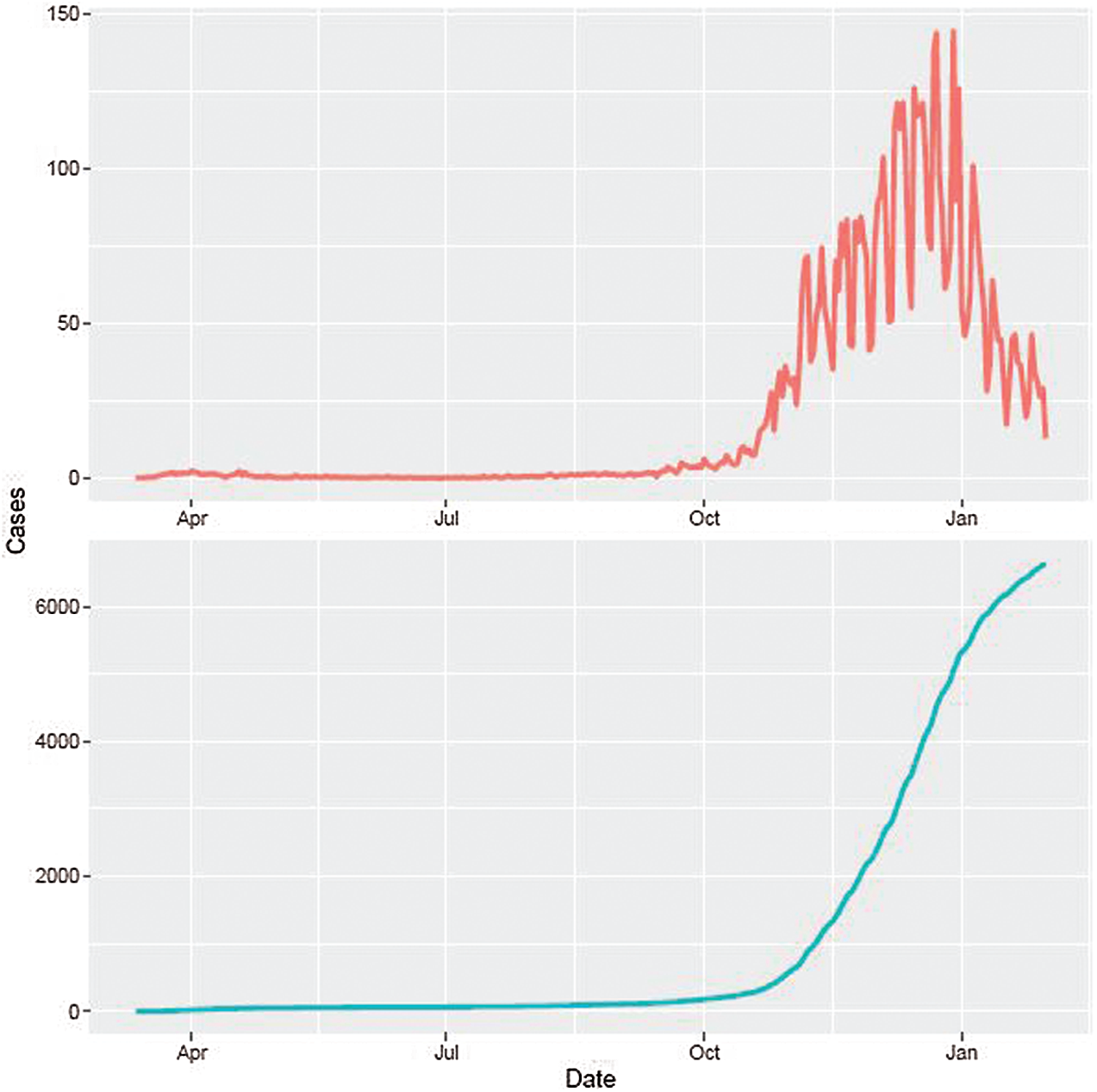
Figure 1: Confirmed (top) and cumulative (bottom) confirmed cases per 100,000 people

Every day by January 26, 2021, forecast models were built based on 35 subsequent observations, and forecasts were performed for 5 steps ahead. As mentioned above, there were different trends in virus spread during the spring and autumn periods, so the authors built models for the spring sub-period by analyzing data for the period from March 12 to June 30, 2020 (the forecast of five steps ahead is included), and for the autumn sub-period from October 1, 2020 to January 31, 2021. We refer to these periods as “first wave” and “second wave” though in epidemiological terms these waves may have different time stamps. The authors do not investigate other sub-periods, since the summer was fairly stable and calm in terms of the spread of COVID-19.

Two approaches were used for the short-term forecasting of confirmed cases of COVID-19 in Lithuania: ARIMA models and the attention-based forecasting method. The results of ARIMA models and all the data used for modeling and forecasting are available at https://www.covid19.projektas.vu.lt.

2.2 ARIMA Model

ARIMA models are frequently used to forecast time series in a short period of time. Although such type of models is simple and easy to apply, these models show good performance for short-term forecasting. ARIMA models are best fitted to stationary or differentiated data if the data is stationary after the differentiation. In this paper, we apply the non-seasonal ARIMA(p, d, q) model:

yt=β+ϕ1yt−1+⋯+ϕpyt−p+θ1εt−1+⋯+θqεt−q,(1)

where t denotes the time; p denotes the order of the autoregressive part (AR(p)); q\; denotes the order of the moving average part (MA(q)); d denotes the order of the differences of the data; yt are the observations that are differentiated d times, usually d = 0, 1, 2; εt are model innovations.

To estimate the ARIMA model, the Hyndman-Khandakar algorithm [24] is used, which combines unit root tests, minimization of the AICc criterion (Akaike information criterion modified for the small samples), and the maximum likelihood estimator. With the view to choose the best model, the AICc criterion has been used. The motivation is related to the fact that a quite small sample of only 35 observations is used in the estimation procedure. The criterion is defined as:

where L^ is the maximum value of the likelihood function of the model, n is a sample size, and k is a number of estimated parameters. More information on the ARIMA models can be found in [25].

2.3 Attention-Based Forecasting Method

The idea of the attention-based approach is to use a mechanism that selects specific factors from the data available. The idea can be accomplished by focusing attention on small regions of multidimensional information rather than on the data as a whole. In this way, dimensionality reduction techniques are used to draw attention to similar countries where the spread of the virus is similar and to further analyze the data for countries that fall into the attention cluster. The attention-based mechanism acts as an extractor of information while inferring the similarity and minimizing the number of countries used for spread forecasting.

The authors propose an attention-based forecasting method that consists of three steps:

Data registration regarding the first confirmed case of COVID-19 for the first wave and the day after July 1, 2020, when the number of confirmed cases per 100,000 is greater than or equal to 3 for the second wave.

Selection of countries most similar to Lithuania, using data mining and machine learning techniques.

Forecasting based on the use of trends in confirmed cases in the selected countries.

Each step of the method is described in more detail in the subsections below.

2.3.1 Data Registration

The outbreak of COVID-19 started at different time periods in different countries. Thus, some countries have a longer history and more historical data of the COVID-19 spread than others. The novelty of the proposed method is to consider the onset of the spread of COVID-19 in different European countries, and to compare the dynamics of the virus and integrate this knowledge into the forecast. The idea is to use data from countries with more historical disease data to forecast trends in Lithuania. For this purpose, we have recorded the data in such a way that the time series starts from the first confirmed case of COVID-19, i.e., we use an artificial time scale (number of days from the first confirmed case) rather than an actual calendar date for the spring sub-period (the first wave). For the autumn sub-period (the second wave), we took data from July 1, 2020, and registered data in such a way that the first day is the day when the number of confirmed cases per 100,000 population is greater than or equal to three. We chose a threshold value of three since the increase in confirmed cases has begun at this time point in the second sub-period for many countries. For the short-term forecasting for the first wave, countries that have more historical data, compared to Lithuania, on the disease from the first confirmed case of COVID-19 were selected: Austria, Belgium, Croatia, Denmark, Estonia, Finland, France, Germany, Greece, Iceland, Italy, Netherlands, North Macedonia, Norway, Romania, Spain, Sweden, Switzerland, and the United Kingdom. Accordingly, the following countries were identified in the same way for short-term forecasting in the case of the second wave: Austria, Belgium, Bulgaria, Croatia, Czechia, Denmark, France, Greece, Hungary, Ireland, Italy, Liechtenstein, Luxembourg, Malta, Montenegro, Netherlands, North Macedonia, Norway, Portugal, Romania, Serbia, Slovakia, Slovenia, Spain, Sweden, Switzerland, and the United Kingdom. Lithuanian data was also included for both waves.

2.3.2 Selection of Countries

The multidimensional data describe complex objects or phenomena characterized by many features. For better comprehension, it is useful to provide data in an easy-to-understand form: to define the structure of the data, relationships, and clusters. Multidimensional data visualization methods are used to provide data mining results in a more comprehensive form by drawing attention to similarities. The attention-based selection of the European Union countries for forecasting is performed by integrating multidimensional data clustering and data dimensionality reduction methods: self-organizing neural network (SOM), multidimensional scaling (MDS), and t-distributed stochastic neighbor embedding (t-SNE). The data was first clustered using the SOM neural network. For the clustering result inspection, visualization techniques such as MDS or t-SNE methods can be used. Different visualization techniques were chosen to validate the clustering results obtained by the SOM, using methods based on different operating principles. Dimensionality reduction methods transform the analyzed dataset from the l-dimensional space Rl into a lower-dimensional space Rd (d<l), where the distribution of points can be observed visually, e.g., d=2. In this study, we consider multidimensional data of the following form:

where n=1,…,35 (number of observations), m—number of countries analyzed, yi1,yi2,…,yin—number of cumulative confirmed cases, xi1,xi2,…,xin—number of cumulative deaths, zi1,zi2,…,zin—number of cumulative recovered cases, p_di—population density for i-th country, respectively, i.e., the study deals with data described by 106 features.

Typically, Yi∈Rl,i=1,…,m are interpreted as points in the multidimensional space Rl, where l defines the dimensionality of the space (in our case, 106 features). If the dimensionality of the projection space is two, then the MDS and t-SNE methods can be applied to represent the multidimensional data in a 2D space.

The self-organizing neural network SOM was used for clustering of multidimensional data. SOM is a neural network-based method that is trained in an unsupervised way using competitive learning [26,27]. Self-organizing maps use a neighboring function to preserve the topological properties of the input space. Typically, SOM represents a set of interconnected neurons according to some topology, e.g., the rectangular SOM is a two-dimensional array of neurons. Each element of the input data set is connected to every individual neuron in the rectangular structure. Every neuron is entirely defined by its location on the grid by its specific index at the row and the column and by its weight (so-called code book vector). After SOM training, the data are presented to SOM, and the winning neuron for each input data is found. The winning neuron is the one to which the Euclidean distance of the input data vector is the shortest. In such a way, the input data are distributed on SOM, and resulting data clusters can be observed. t-SNE is a nonlinear dimensionality reduction technique based on Stochastic Neighbor Embedding [28]. The method minimizes the divergence between two distributions: a distribution that measures pairwise similarities of the high-dimensional objects and a distribution that measures pairwise similarities of the corresponding low-dimensional points in the embedding.

The MDS method is used to find a configuration of points in a space, usually Euclidean, where each point represents one of the objects or individuals, and the distances between pairs of points in the configuration match as well as possible the original dissimilarities between the pairs of objects or individuals [29]. The MDS method represents (dis)similarity data as distances in a low-dimensional space to make these data accessible to visual inspection and exploration [30].

2.3.3 Forecasting

The trends of the number of confirmed cases in the countries which belong to the same cluster as Lithuania and have more historical data on the disease from the first confirmed case of COVID-19 are used. The regression models with countries as covariates are considered. The forecasting is done for such a number of days ahead as is the history of the confirmed number of cases in the countries belonging to the same cluster as Lithuania. However, some countries, which belong to the same cluster as Lithuania, do not have a much longer history of confirmed cases than Lithuania. Thus, to obtain a forecast for required steps ahead, ARIMA models (see Section 2.2) were used to forecast the number of the confirmed cases in each country, and then these forecasts were employed in regression analysis to get the forecast of the confirmed cases in Lithuania.

To achieve the goal above, the linear regression with ARMA errors was used:

yt=β0+β1xt+ηt,ηt=∑i=1p⁡ϕiηt−i+εt+∑j=1q⁡θjεt−j, (2)

where pand q are AR and MA orders respectively; β0, β1, ϕi, θj are unknown parameters and εt are random errors.

After the linear regression models were obtained for each country in the cluster, the forecast was calculated by taking the average of forecasts from these models:

y^LT;t=1k∑l=1k⁡y^l;t,(3)

where y^l;t is the forecast from each regression performed.

2.4 Forecast Accuracy

The comparison of the accuracy of the forecasts over the considered time period was made by choosing models for every interval of 35 days and forecasting five steps ahead. The following measures of the forecast accuracy were used:

RMSE=1T∑i=1T⁡(y^t−yt)2,MAPE=100T∑i=1T|yt−y^tyt|,MAE=1T∑i=1T|yt−y^t|(4)

where T is the number of time points, yt and y^t are observed and fitted values of the dependent variable, respectively.

3  Results

3.1 ARIMA Forecasting Results

We estimate the ARIMA model for cumulative confirmed cases every day with 35 recent observations for the period March 12, 2020–January 26, 2021, dividing data into two sub-periods as follows: March 12–June 25, 2020, and October 1, 2020–January 26, 2021. Earlier data and the summer period are truncated due to a very small number of confirmed cases.

We would like to point out that modeling started at the end of March, and different types of models and lengths of data at first were used. Here we present the final version of the forecasting approach, thus the historical forecast in the paper might differ from the forecast announced for the public.

Note that the model was built based on the cumulative number of confirmed cases per 100,000 people. In addition, the authors analyze the non-seasonal ARIMA model for the daily data, though a slight seasonality might be observed because of the weekend effect, when fewer tests are performed. However, testing with the seasonality models does not have better performance than with the non-seasonal models.

A new ARIMA model is fitted for every day. The orders of each ARIMA model are shown in Fig. 2.

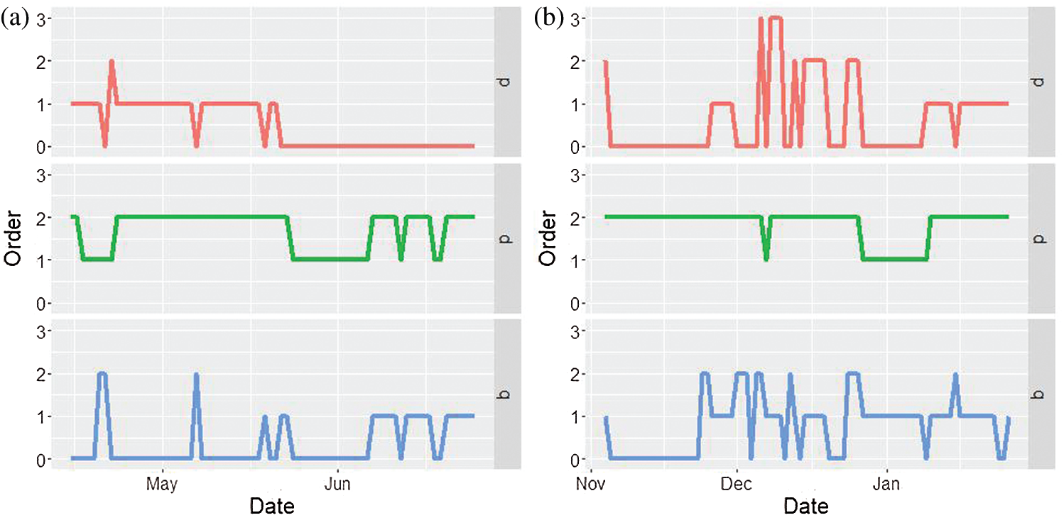
Figure 2: ARIMA orders for every day models. (a) March 12–June 25, 2020 (b) October 1, 2020–January 26, 2021

For every day, not only a new model is built, but forecasts are performed for five steps ahead as well as prediction intervals with 80% and 95% prediction probabilities are computed.

The complete algorithm for every day model is given in Algorithm 1 presented in Fig. 3.

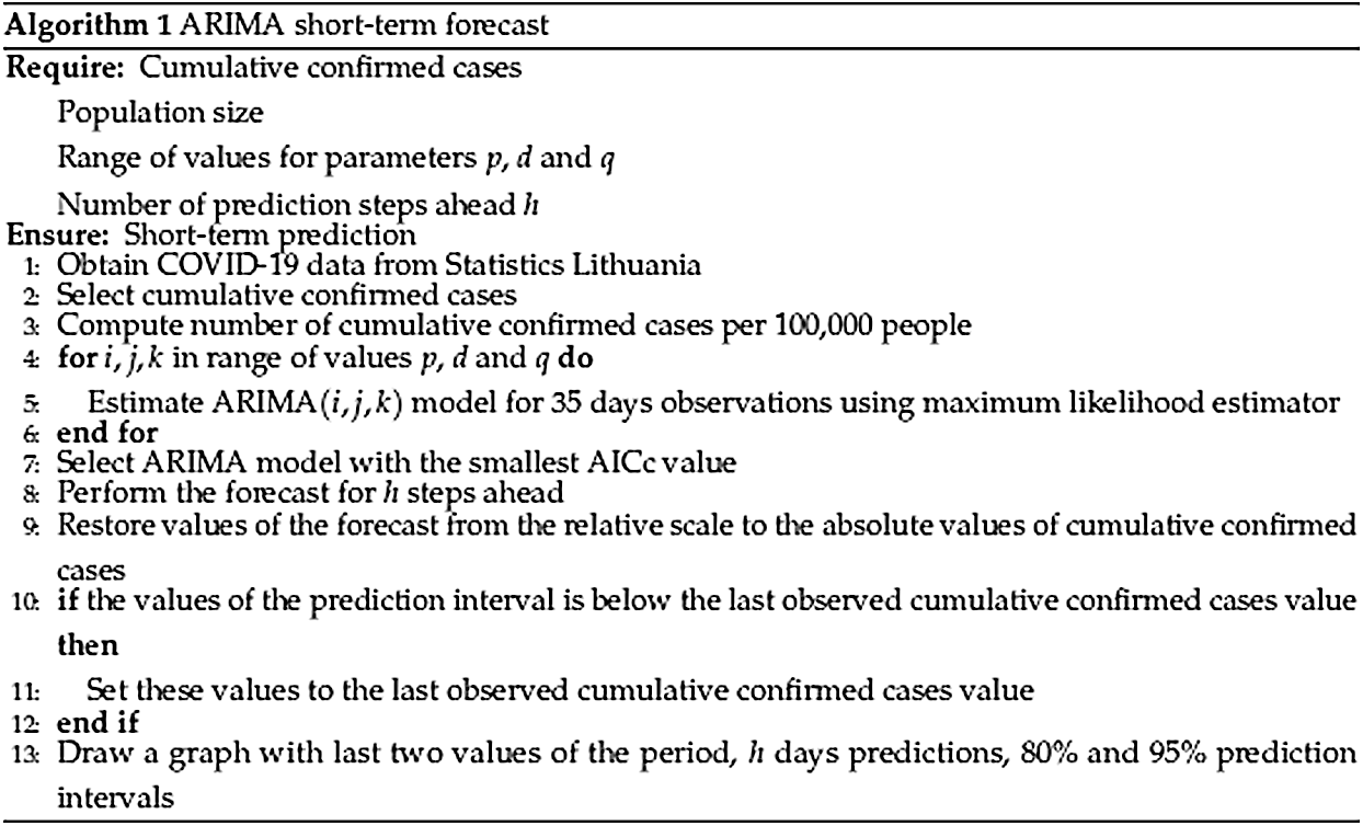
Figure 3: Algorithm 1. ARIMA short-term forecast

The result of Algorithm 1 is the graph where the black line and black dots indicate predicted values, the red dots indicate true values, the dark blue band indicates the 80% prediction interval, and the light blue band indicates the 95% prediction interval (see Fig. 4).

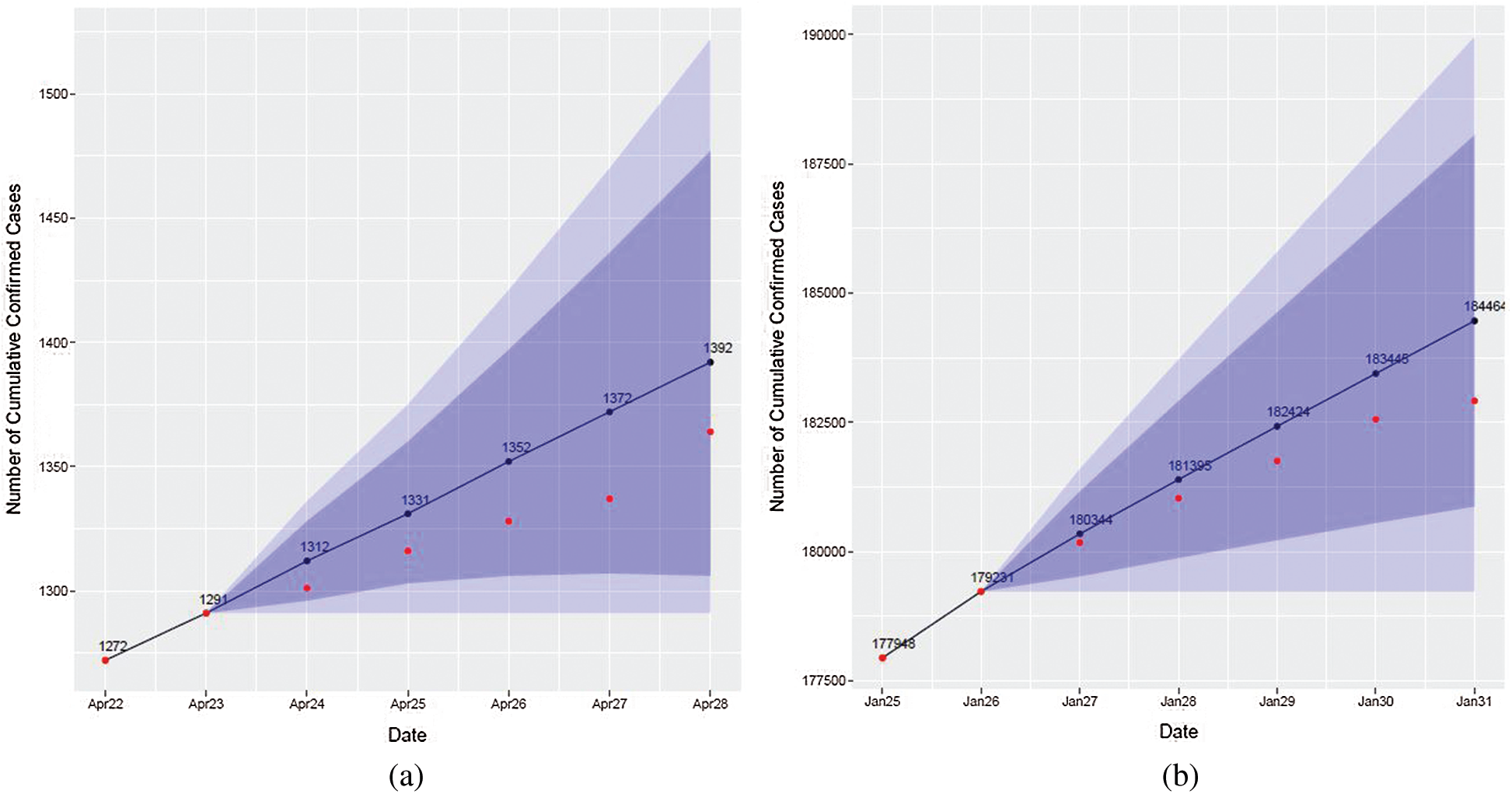
Figure 4: Visualization of forecasting results obtained by ARIMA. Red dots represent actual cases, blue line and dots represent ARIMA forecasts, and the blue and light blue bands are prediction intervals. (a) April 22–April 28, 2020 (b) January 25–January 31, 2021

As it was mentioned earlier, the historical data has been changing over time, and the prediction scheme has also slightly changed over the pandemic period. Thus, a retrospective analysis of the goodness of the prediction of the ARIMA models has been accomplished. To achieve this goal, training set errors and prediction errors computed over the whole period, taking into account all historical models, were investigated (see Fig. 5: Algorithm 2).

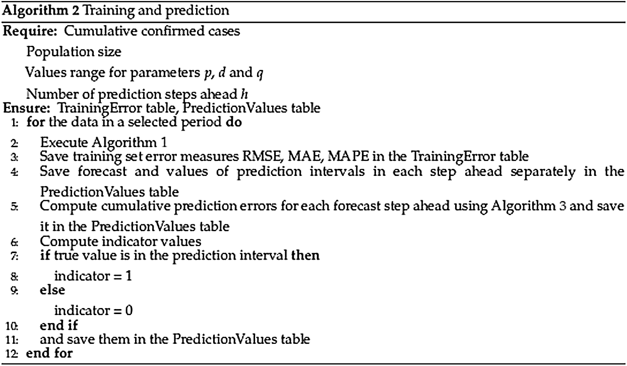
Figure 5: Algorithm 2. Training and prediction

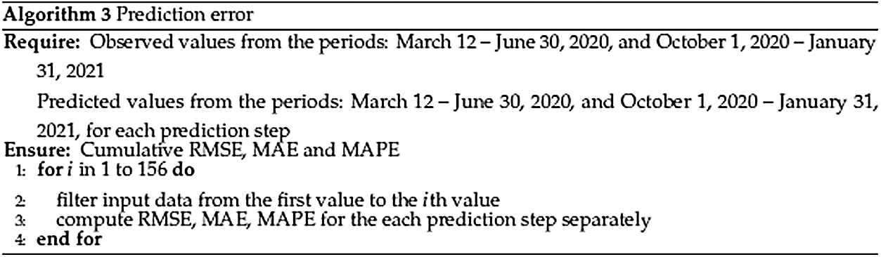
Figure 6: Algorithm 3. Prediction error

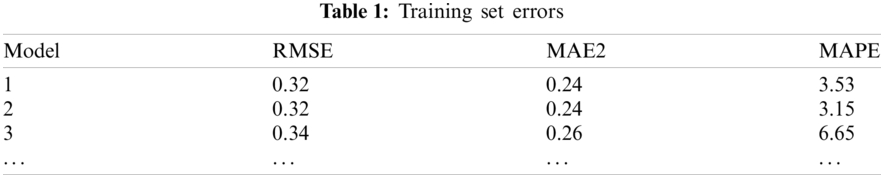
In total, 156 models (72 for the first wave and 84 for the second wave) were estimated, and training sets and prediction errors were saved and the final output of Algorithm 2 consists of two tables. Tab. 1 illustrates several TrainingError values.

The result of a Prediction Values table is a table with 52 columns and 77 rows for the first wave and 89 rows for the second wave. The columns are as follows:

•   Date: the date for the true and predicted values;

•   Observed: the observed values;

•   S1_point, … , S5_point: point forecasts for each step ahead separately computed with Algorithm 1;

•   S1_l80, … ,S5_lo80, S1_hi80, … ,S5_hi80, S1_lo95, … ,S5_lo95, S1_hi95,…S5_hi95: prediction intervals lower and upper values computed with Algorithm 1;

•   RMSE_S1, … ,RMSE_S5, MAE_S1, … ,MAE_S5, MAPE_S1, … ,MAPE_S5: cumulative prediction errors computed with Algorithm 3;

•   S1_int_80, … ,S5_int_80, S1_int_95, … ,S5_int_95: indicator values, if true value is in the prediction interval.

The cumulative RMSE, MAE, and MAPE errors showed that the values of the median and variance increased with each prediction step (see Fig. 7, e.g., with MAPE error).

The same algorithms have been applied for the second period of data, as mentioned in SubSection 2.1: October 1, 2020–January 31, 2021.

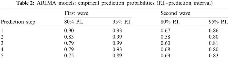
The results obtained are very similar, but we have slightly larger errors. The bigger difference appears in the empirical probability for the true value to be in the prediction interval. Note that the authors have computed 80% and 95% prediction intervals, but retrospectively it is the indicator values if the true value is in this interval (Algorithm 2). Empirical prediction probabilities were computed as follows:

The results are presented in Tab. 2. It can be seen that the results of the forecast are promising. For the further prediction steps, the probability is getting lower but is still above the value of 0.89 for the step 5 with the 95% prediction interval over the first wave and greater than 0.80 for the second wave.

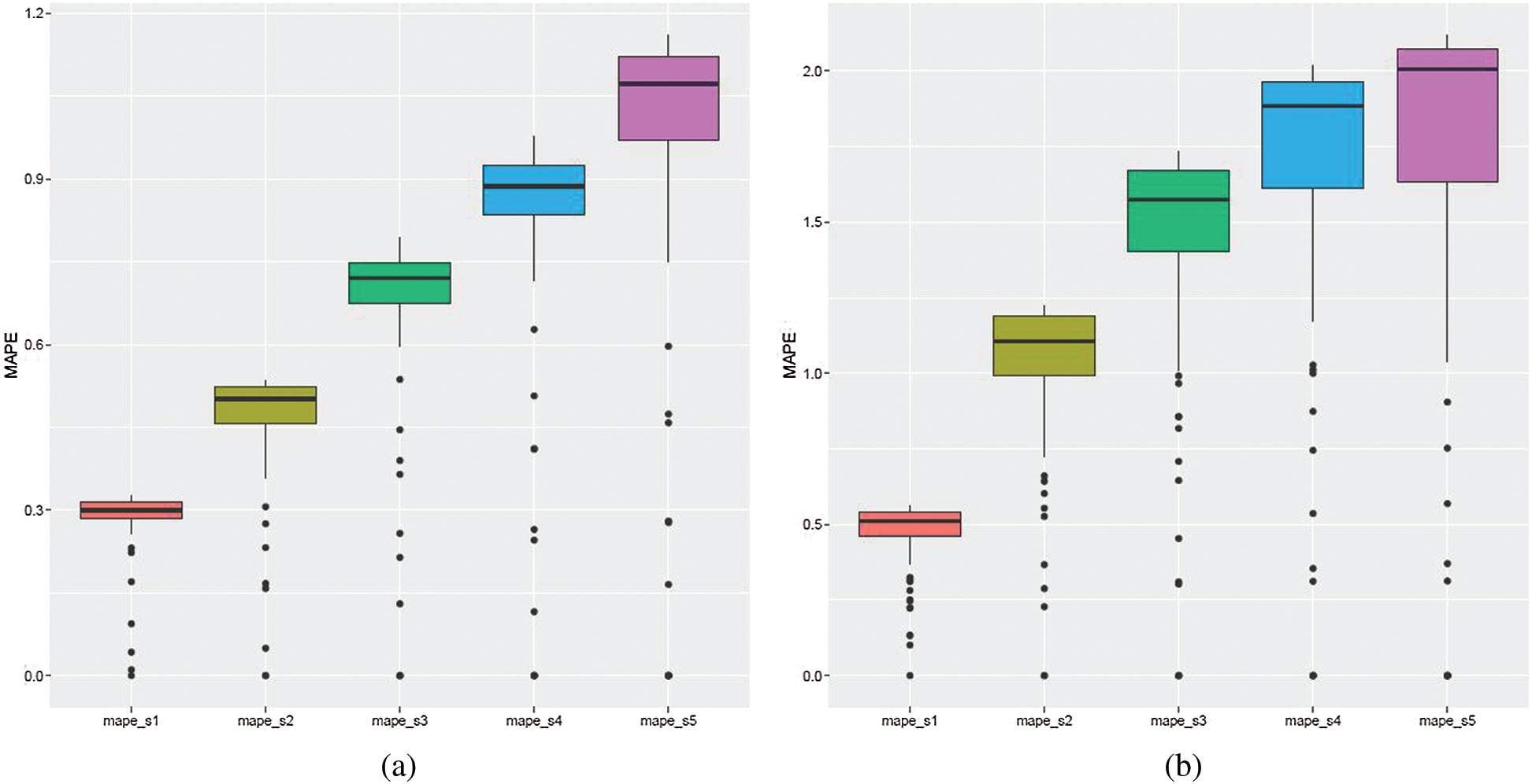
Figure 7: ARIMA models: cumulative MAPE errors. The figure shows boxplots for each prediction step, from one to five, ahead, that is mape_s1 denotes MAPE values for the first step ahead forecast, mape_s2 denotes MAPE values for the second step ahead forecast, etc. (a) March 12–June 30, 2020 (b) October 1, 2020–January 31, 2021

3.2 Attention-Based Forecasting Results

The results obtained using attention-based forecasting are presented in this section. The complete scheme for attention-based forecasting is given in Algorithm 4 (see Fig. 8). In an effort to compare the resulting forecasting accuracy of the two methods considered, the time periods, measures of the forecast accuracy, and the study of performance over the time kept the same as in Algorithms 2 and 3 (see Figs. 5 and 6).

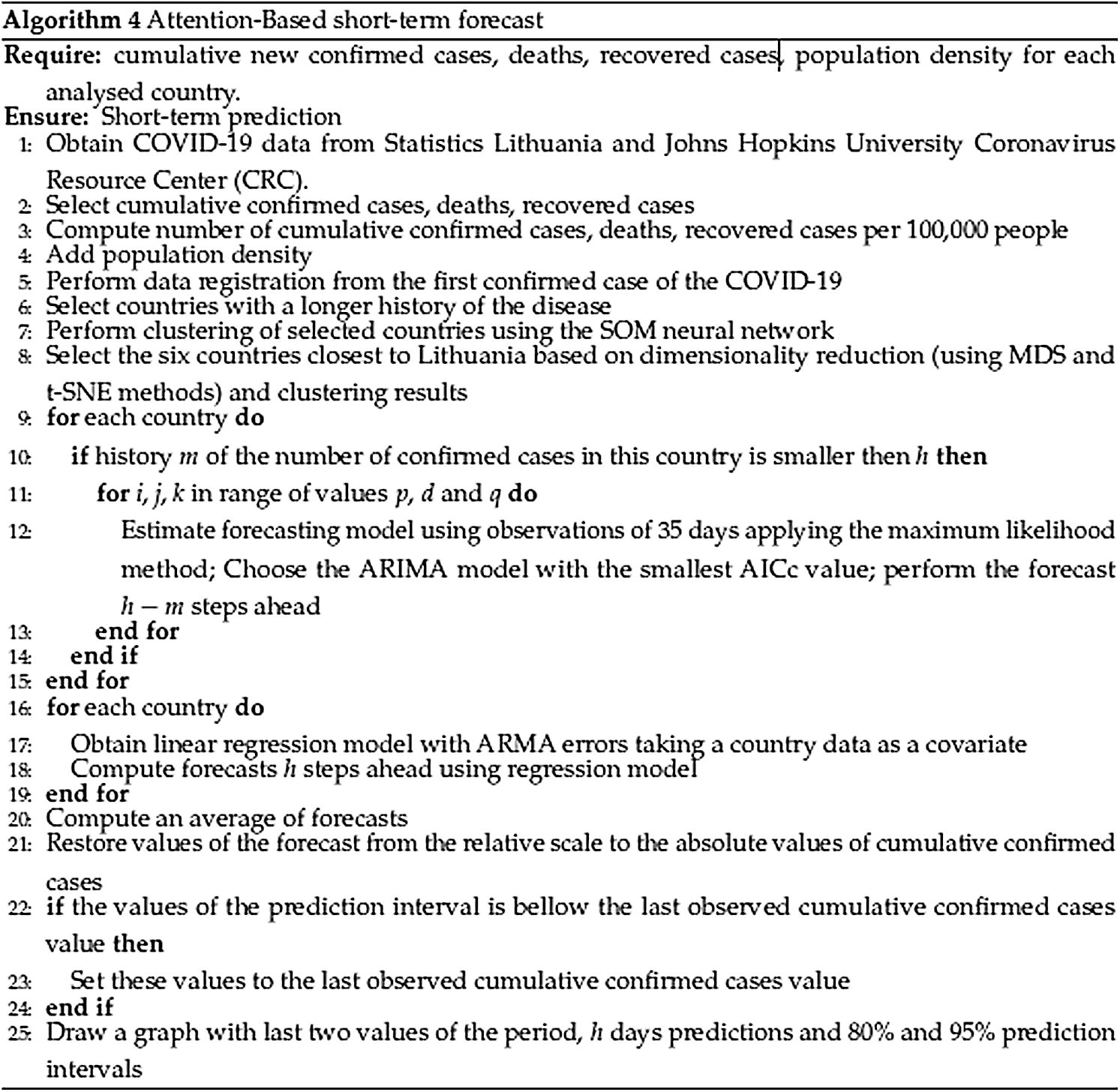
Figure 8: Algorithm 4. Attention-based short-term forecast

3.2.1 Registration and Clustering Results

Following the data registration described in Section 2.3.1, 20 European countries with a longer history of the disease and virus spread than Lithuania were selected for the study: 17 European Union countries, the United Kingdom, Norway, and Northern Macedonia. Daily cumulative relative data (per 100,000 people per day) for the last 35 days of the research is used: cumulative new confirmed cases, deaths, recovered cases, and population density. As mention above, the multidimensional data consists of 106 features per country. Following the registration of data for the first case (see Section 2.3.1), a cluster and visual analysis of multidimensional data were carried out (see Section 2.3.2). To forecast the number of cases and disease trends in Lithuania, six countries were identified with more historical disease data, and in which the registered data for the past 35 days have a similar trend to Lithuania. Tab. 3 presents the six countries selected for regression analysis for each month from March to June (registered for the first wave), which have been identified as most similar countries to Lithuania in terms of trend and similarity of the virus spread. The countries were ranked based on the summarized results of visual and cluster analysis (see Section 2.3.2). All six selected countries had a longer history from the first confirmed case of COVID-19 compared to Lithuania based on SOM output. In some cases, SOM output resulted in less than six countries in the same cluster as Lithuania. To select the lacking data to form the cluster of six countries, the points closest to Lithuania, representing the countries, were identified based on Euclidean distances in the multidimensional space.

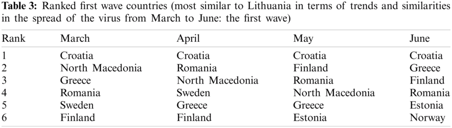
Tab. 3 shows that Croatia, Northern Macedonia, Romania, and Greece were the most similar countries to Lithuania in terms of virus spread trends from March to June. Since the visualization results obtained by the MDS and t-SNE methods are quite similar, we present only the results obtained by the t-SNE method. The visualization results of the analyzed data from the period from March 12 to April 15, 2020 are presented in Fig. 9a. When visualizing data, one color is allocated to countries in a single cluster, formed using the SOM. Similar trends in the spread of the virus during this period were also observed in Sweden, Finland, Estonia, and Norway, based on the results of visualization of the corresponding multidimensional data (see Fig. 9). As the situation in Romania and Macedonia changed already in May, these countries began to disappear from the cluster with Lithuania. The summer period is a stable and calm time in the spread of COVID-19, the situation changes slightly. Lithuania belongs to the same cluster as countries with a small number of confirmed cases. From August to September, the same cluster with Lithuania included Greece, Finland, Estonia, Norway, and Germany.

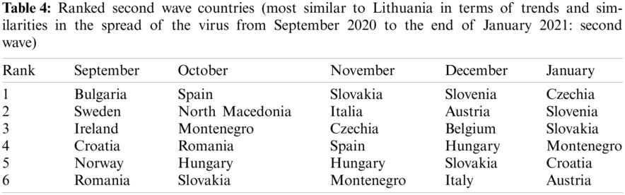
However, since November, the situation begins to change. Tab. 4 presents six countries from September to January (data registration for the second wave). From November, Lithuania was in the same cluster as Slovenia, Czechia, Slovakia, Austria, Italy, Montenegro, and Hungary. The number of cases in these countries has been increasing. As an example, the results of the visualization of the analyzed data in the period of December 23, 2020–January 26, 2021, obtained using the t-SNE method, are presented in Fig. 9b. The same clustering results were observed by applying the MDS method for clustering results inspection. However, MDS relies on Euclidean distances in multidimensional space, and when the figures are produced in 2D space, the points representing countries form quite dense clusters on the plane that are hardly readable but comparable to those obtained by t-SNE. Thus, only t-SNE results are being presented. Lithuania has been a part of the same cluster as Czechia, Slovenia, and Luxembourg. Other countries (Austria, Slovakia, Croatia, Montenegro, Hungary, Italy) have been identified as similar to Lithuania, although they belong to other clusters.

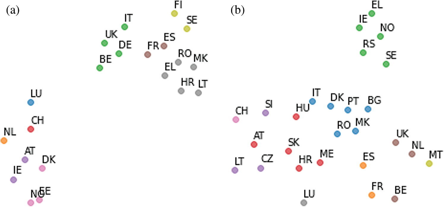
Figure 9: Visualization results obtained using t-SNE. Countries with the same color depict the same cluster meaning a similar COVID-19 spread. European Union and other countries have been assigned a two-letter country code.3 (a) March 12–April 15, 2020 (b) December 23, 2020–January 26, 2021

3.2.2 Forecasting Results

The approach outlined in Section 2.3.3 and the results presented in Section 3.2.1 were used to obtain the forecasts. Six countries from the same cluster and closest to Lithuania were used to make forecasts based on the number of cumulative confirmed cases. The same time intervals were considered to compare the results with those of the ARIMA models: the first is March 12–June 30, 2020 (corresponds to the first wave of COVID-19), and the second is October 1, 2020–January 31, 2021 (corresponds to the second wave).

Algorithm 4 was applied to obtain results, and the graph presents the final result (see Fig. 10): the black line and black dots represent the predicted values, the red dots represent true values, and the dark and light blue bands represent 80% and 95% prediction intervals, respectively.

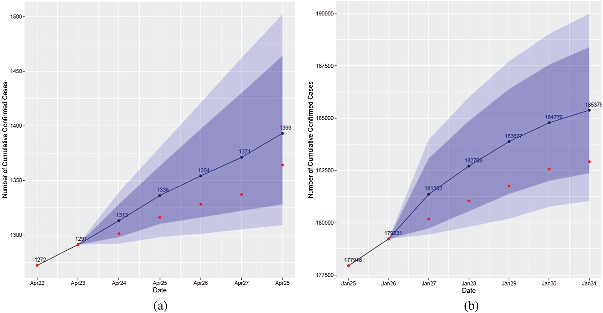
Figure 10: Visualization of forecasting results obtained by the attention-based method. The red dots represent actual cases, the blue line and dots represent forecasts using the attention-based method, and the blue and light blue bands are prediction intervals. (a) April 22–April 28, 2020 (b) January 25–January 31, 2021

Comparing the results of ARIMA models and attention-based forecasting (see, for example, Figs. 3 and 10), it can be concluded that one of these methods shows a better fit for some periods and the other is better for other periods. A higher forecast accuracy is achieved in periods when countries in the same cluster are closer to Lithuania.

All models, as in the case of ARIMA models, were estimated historically (overall 156 models were fitted: 72 in the case of the first wave and 84 in the case of the second wave), training set errors were saved and prediction errors over the two considered sub-periods were obtained (see Fig. 5: Algorithm 2). The cumulative values of RMSE, MAE and MAPE (see Fig. 6: Algorithm 3) show that the median and variance become larger with each prediction step (see Figs. 11a and 11b for MAPE values). The medians are similar, as in the case of ARIMA, however, the variance is slightly larger.

The comparison of the results obtained by the attention-based method for the two sub-periods (waves) shows that the forecast errors in the case of the first wave (see Fig. 11a for MAPE values) are smaller than in the case of the second wave (see Fig. 11b). This is due to the reason that the situation in countries differs more in the autumn than in the spring when countries from the same cluster as Lithuania were closer to each other.

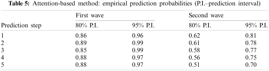
The empirical probabilities that the true value is in the prediction region were obtained (see Tab. 5). The results show that the accuracy of the estimation is similar to that of ARIMA in the case of the first sub-period (wave) considered, but it is slightly worse in the case of the second wave.

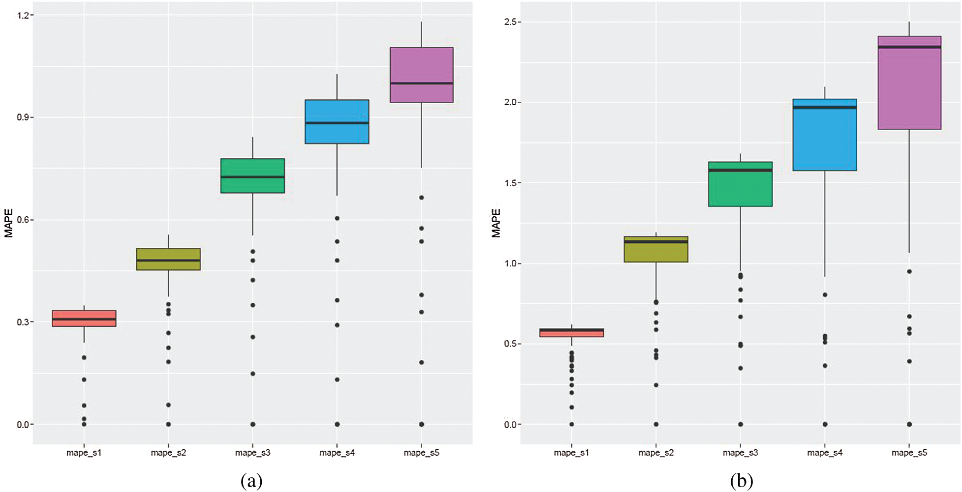
Figure 11: Attention-based method: cumulative MAPE. The figure shows boxplots for each prediction step one through five, ahead, that is mape_s1 denotes MAPE values for the first step ahead forecast, mape_s2 denotes MAPE values for the second step ahead forecast, etc. (a) March 12–June 30, 2020 (b) October 1, 2020–January 31, 2021

4  Discussion

This study investigates methods for obtaining short-term forecasts of the COVID-19 virus spread that can be useful for policymakers and public institutions in making necessary decisions and providing useful guidance as to what might happen in the coming week. By borrowing the idea of the attention-based approach from Long Short-Term Memory deep neural networks and combining this approach with the mathematical modeling and prediction methods, we obtain a powerful tool for understanding the spread of COVID-19 and exploring different short-term spread scenarios.

Two approaches were used for short-term forecasting of the confirmed COVID-19 cases in Lithuania: the ARIMA model and a new attention-based forecasting method, which combines machine learning techniques and statistical methods. The novelty of the approach presented above is the use of data from countries with a longer history of the disease to forecast trends in Lithuania. To this end, the authors introduce the data registration from the first confirmed case of COVID-19. Such a way of data registration and integral data analysis using techniques for clustering and multidimensional data dimensionality reduction allows to assess trends in the spread of the virus in different countries and to group them according to similarity, i.e., to draw attention to those countries where the spread of COVID-19 behaves in a similar way. Moreover, the proposed approach allows to assess the dynamics of the spread of the virus and changes in the situation over time. The clustering analysis shows the specificity of the virus spread and enables to review the measures applied in the countries of the same cluster to control the virus and assess the impact (effectiveness) of the measures applied on the increase in the number of newly confirmed cases of the disease. The attention-based focus and identification of countries that are similar to the investigative one, i.e., Lithuania, with the ability to have a longer history of virus spread analysis, as well as the forecast based on their trends, allows to create and foresee the virus spread scenarios based on the historical data of other countries.

Summarizing the results of the forecasting, it can be concluded that both methods demonstrate similar accuracy in forecasting of the so-called first wave time period COVID-19 cases (March 12–June 30, 2020), none of the methods outperforms the other. The forecast accuracy obtained using the attention-based forecasting, taking the second wave (October 1, 2020–January 31, 2021), is slightly lower compared to the results obtained by ARIMA. The explanation can be related to the fact that the situation and trends of confirmed cases in the countries being rather different, the number of countries in the same cluster as Lithuania is not large, and the distances from Lithuania in the cluster are varied. However, the attention-based forecasting approach gives promising results. Higher forecast accuracy is achieved in periods when the countries in the same cluster are closer to Lithuania. The two approaches discussed above complement each other and provide insights for the short-term forecasting of COVID-19 spread and enable to validate the forecasting results. The dimensionality reduction techniques, viewed as an attention-based method for similar COVID-19 spread country or region selection, combined with regression analysis, provide a means to validate the forecasting results. The approach presented in the paper can be applied to any country with the view to analyze other pandemic situations.

Acknowledgement: The authors are thankful for the high-performance computing resources provided by the Information Technology Open Access Center at the Faculty of Mathematics and Informatics of Vilnius University Information Technology Research Center.

Funding Statement: This project has received funding from the Research Council of Lithuania (LMTLT), agreement No S-COV-20-4.

Conflicts of Interest: The authors declare that they have no conflicts of interest to report regarding the present study.

1https://osp.maps.arcgis.com/apps/MapSeries/index.html?appid=c6bc9659a00449239eb3bde062d23caa.

2https://github.com/CSSEGISandData/COVID-19.

3https://ec.europa.eu/eurostat/statistics-explained/index.php/Glossary:Country_codes.

This work is licensed under a Creative Commons Attribution 4.0 International License, which permits unrestricted use, distribution, and reproduction in any medium, provided the original work is properly cited.