DOI:10.32604/cmc.2022.018268
| Computers, Materials & Continua DOI:10.32604/cmc.2022.018268 | |
| Article |
Multiscale Image Dehazing and Restoration: An Application for Visual Surveillance
1Department of Computer Science, COMSATS University Islamabad, Wah Campus, 47040, Pakistan
2Department of Computer Science, COMSATS University Islamabad, Lahore Campus, Lahore, Pakistan
3Department of Electronics and Communication Engineering, Hanyang University, Ansan, Korea
4Department of ICT Convergence, Soonchunhyang University, Asan, 31538, Korea
5Department of Computer Science, HITEC University Taxila, Taxila, 47080, Pakistan
*Corresponding Author: Yunyoung Nam. Email: ynam@sch.ac.kr
Received: 02 March 2021; Accepted: 03 April 2021
Abstract: The captured outdoor images and videos may appear blurred due to haze, fog, and bad weather conditions. Water droplets or dust particles in the atmosphere cause the light to scatter, resulting in very limited scene discernibility and deterioration in the quality of the image captured. Currently, image dehazing has gained much popularity because of its usability in a wide variety of applications. Various algorithms have been proposed to solve this ill-posed problem. These algorithms provide quite promising results in some cases, but they include undesirable artifacts and noise in haze patches in adverse cases. Some of these techniques take unrealistic processing time for high image resolution. In this paper, to achieve real-time halo-free dehazing, fast and effective single image dehazing we propose a simple but effective image restoration technique using multiple patches. It will improve the shortcomings of DCP and improve its speed and efficiency for high-resolution images. A coarse transmission map is estimated by using the minimum of different size patches. Then a cascaded fast guided filter is used to refine the transmission map. We introduce an efficient scaling technique for transmission map estimation, which gives an advantage of very low-performance degradation for a high-resolution image. For performance evaluation, quantitative, qualitative and computational time comparisons have been performed, which provide quiet faithful results in speed, quality, and reliability of handling bright surfaces.
Keywords: Dehaze; defog; pixel minimum; patch minimum; edge preservation
Haze is a collection of dust and smoke particles that are scattered in the air. Haze is an atmospheric phenomenon that reduces outdoor scene prominence. From low-level image analysis to high-level object recognition, most computer vision algorithms assume that the input image is haze-free. Therefore, haze removal is a prerequisite for many practical applications.
Most of computer vision and computer graphic application use image formation model [1–5] to describe the hazy image:
where I(x) is hazy image, J(x) is scene radiance, A is airlight and t(x) is transmission or visibility map of an image. In literature, properties of airlight are commonly assumed to be constant across a scene [1–4,6], which is often assumed to be the brightest point of an image or sky. Transmission value t(x) is a visibility of an object that reaches the camera, inversely proportional to the depth of the scene d(x) and number airborne particles represents as β. Single image dehazing is always been a under constraint problem and to solve this under constraint problem different assumption were made by prior algorithms. These dehazing algorithms can mainly categorize into two key points: i) additional information based transmission estimation e.g., multiple hazy images under different weather conditions [7] or by using different polarization filter [8] or by using near infra-red channel [9] or by given depth map of hazy image [10] and ii) single image dehazing, more practical solution. In single image dehazing, most methods estimate depth map using different statistical and experimental assumptions [1–3,6,10–12]. These approaches can further be categorized methods that need some user input [10–12] and automatic methods [1–3,6].
Recent works focus on single image dehazing methods. This is quite challenging problem with fewer information and multiple assumptions. Some sate of art algorithms are discussed in this section. Fattals [3] assume that target surface shading and transmission are partially uncorrelated and by using the independent component analysis (ICA) transmission map was estimated. Fattal [6] presented another dehazing algorithm that is based on images generic regularity in which image pixels typically exhibit a one-dimensional RGB color space, this algorithm is known as color-lines. Berman et al. [13] creates haze lines for each color cluster in RGB space.
Recently, some works has been done to improve the process of dehazing using machine learning framework. Tang et al. [14] investigate and combine four types of haze-relevant features in a Random Forest [15] based regression framework. They found that the dark-channel is the most informative feature in learned regression model it confirms the observation of He et al. [2] from a learning perspective, while other haze-relevant features also contribute significantly in a complementary way. Zhu et al. [16] estimate depth map of a hazy image by presenting a linear model for depth estimation, prior of color attenuation. Parameters are selected using supervised learning. Basic observations of color attenuation prior are that the brightness and the saturation of pixels in a hazy image vary sharply along with the change of the haze concentration and the hazy regions are characterized by high brightness and low saturation. Cai et al. [17] presented “DehazeNet” in which medium transmission is estimated using Convolutional Neural Networks (CNN). Dehazing algorithms [7,8] were proposed that presents an energy function, which is minimized or maximized to derive a numerical scheme. Nishino et al. [8] proposed a Bayesian probabilistic dehazing algorithm for depth estimation and scene radiance from a single foggy image using factorial Markov random field. Meng et al. [7] proposed an effective dehazing algorithm by using the inherent boundary constraints.
State of the art dark channel prior (DCP) [2] is a generalization of dark-object subtraction method [18]. DCP is a simple but effective image prior. Recent works [1,19–21] focus more on improving the shortcoming of DCP to achieve real-time halo-free dehazing. Yu et al. [1] proposed a block-to pixel interpolation method, which is a weighted voting method to generate fine transmission map. Gibson and Nguyen [22] calculate the effectiveness of DCP by using use minimum volume ellipsoid approximation and principal component analysis. Latter unlike DCP, they proposed dehazing algorithm [20] to calculate patch minimum for darkest pixel in each ellipsoid. Further to speed up the haze removal process Median filter [23] was also suggested. Matlin et al. [24] combined the dark-channel approach with nonparametric denoising. They suggested that every image has noise due to sensor errors and dehazing process can amplify the sensor noise.
Dark channel prior was proposed on concept of dark pixels in haze free images and states that mostly non-sky regions of haze free outdoor images has at least one color channel intensity close to zero. Pixel minimum Ic of an image represent minimum value of each pixel across RGB channels.
Patch minimum of these non-sky regions they will tends to zero.
Normalizing A on both side of Eq. (1).
As per DCP, Jdark tends to zero, so direct attenuation term should be zero.
where ω is a constant term whose value should between0 ≤ ω ≤ 1. Purpose of this constant is to avoid transmission to be zero and also to keep small amount of haze in image to keep its natural look. For final dehaze image:
To remove low intensity noise in transmission map a lower limit T of transmission is set, whose value should betweenT ≤ t(x) ≤ 1.
Dark Channel Prior Shortcomings: Dark channel prior DCP has still not been utilized to its full potential. It has been observed that DCP have two main shortcomings.
i) DCP assumes that transmission map
ii) DCP basic concept of dark channel Jdark assumes that in a haze free image there must be dark pixel in every patch. This concept fails in case of large bright surfaces i.e., white wall or snowy ground and over saturates these bright surfaces during dehazing.
These shortcomings are due to inaccurate transmission map estimation. In DCP [2] transmission map is calculated using patch minimum Imin operator. Patch minimums can be estimated with multiple patch sizes, from small to large with their own advantages and disadvantages. For large size patch minimum, bright surface handling capabilities improves as their chances to find dark pixel in larger window increases but also results in poor edge preserving properties i.e., if patch minimum is computed at bright side object boundary and its minimum value is located at dark side of object boundary their transmission value is inaccurately estimated lower than its actual value. These results in inaccurate edge perversion properties and unwanted haloes near object boundaries. Similarly for small size patch minimum, there are better edge perversion properties but poor bright surface handling capabilities i.e., for large bright object larger than patch size with no dark pixel its patch minimum results in very high value and considering this object as haze and results in oversaturated dehaze image.
From these observations it can be concluded that performance of DCP method [2] is highly affected by selected patch size. If larger patch size is selected bright surface handling capability of DCP will be improved but it is not edge preserving causing haloes around object boundaries. Similarly if smaller patch size is selected DCP will be edge preserving but has poor bright surface handling capabilities, results in over saturated patches on large white objects.
In this paper, proposed novel framework for single image dehazing and to improve shortcoming of DCP efficiently by estimating transmission map with edge preserving and reduced texture noise properties. As discussed, performance of DCP is highly affected by patch size so, instead of using single patch minimum the proposed algorithm combines multiple sized patch minimums to achieve properties of edge preserving and halo free dehazing. Smoothing and edge preservation properties of fast guided filter were also used to improve the quality of dehazing and to reduce texture noise. For high resolution images an efficient scaling technique is used, this will significantly reduce processing time with no visual degradation and very small processing time change.
The rest of this paper is organized as follows. Our proposed method is presented in Section 3. The experimental results and analysis are shown in Section 4. Finally, the conclusions are given in Section 5.
In this paper, proposed a fast and an effective technique of single image dehazing. Our main focus is to handle DCP shortcomings gracefully and to improve performance for high resolution images. By observing prior algorithms [1–3,6,14] generic dehazing algorithms can be divided into three major step 1) Airlight estimation 2) transmission map estimation and refinement 3) Image dehazing. Generic dehazing model can be seen in Fig. 1. Airlight A and Image dehazing (using Eq. (7)) were accurately estimated by prior algorithm so, transmission map estimation and refinement defines efficiency and performance of dehazing algorithm.
Most of the haze removal algorithms assume that the atmospheric light is a constant 3D vector in input hazy image that can be estimated by finding brightest point of an image. In proposed technique, airlight is estimated by taking 0.1% brightest points in the dark channel of an image then choose a point with maximum intensity [21]. The brightest point of an image, when used this method, can be brighter than air light. This can be easily identified as for it:
This makes the transmission value negative for the surfaces that are brighter than A, so,
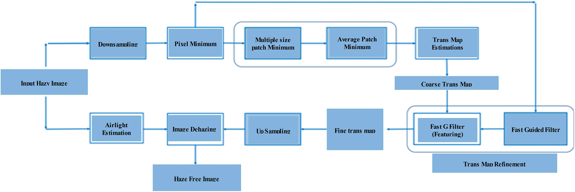
Figure 1: Flow diagrams of our proposed method Multiscale Image Dehazing
Similarly, transmission value can approach to zero for large bright surface where patch minimum does not find any dark pixel or it can be negative if airlight A inaccurately estimated and local pixel has greater value. This results in over dehazing cause dark round artifacts in sky region. For such regions He et al. [2] sets minimum limit of transmission τ0 = 0:1.
Setting minimum value of transmission τ0 is critical, if selected value is too low it fails to remove unwanted dark round artifacts and if value is too high it will result in poor dehaze image. To handle such large bright surface a simple but effective method using multiple patch size is proposed that will reduce the contrast of bright region having values greater than airlight. Using Eq. (1), the transmission can be derived.
3.2 Transmission Map Estimation
Transmission map estimation defines performance and efficiency of dehazing algorithm. The multiscale patch minimum have better edge preserving properties and bright surface handling capabilities as it can be observed in Fig. 2a with different patch sizes as shown in Fig. 3 twenty different patch sizes are generated and red marking at top right and at left bottom of an image show inaccurately estimated bright surfaces by DCP.
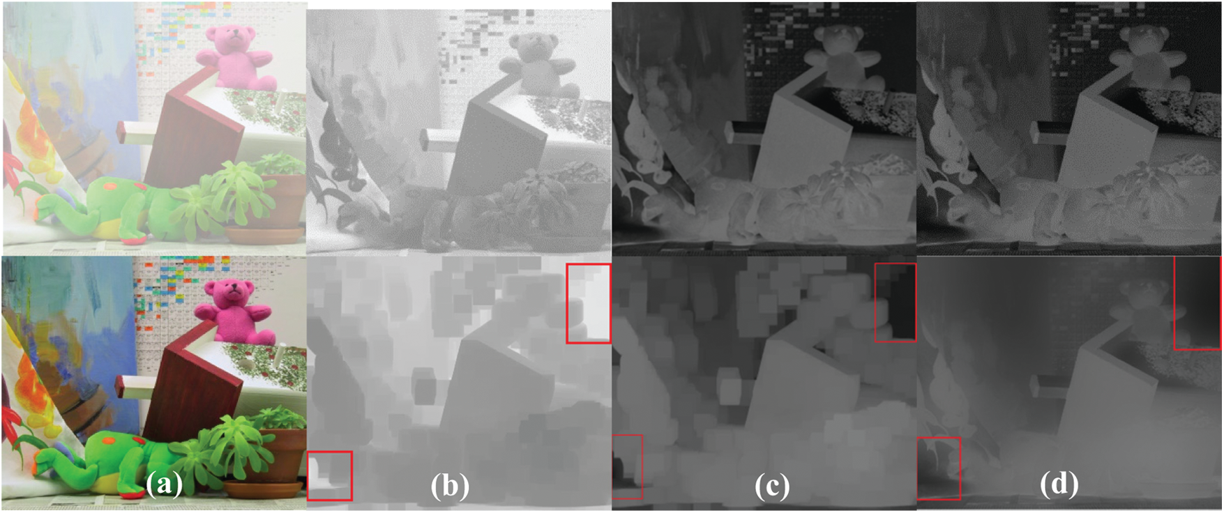
Figure 2: Pixel minimum and transmission map estimation. (a) The hazy image as input and the ground truth image. (b) The pixel minimum and patch minimum. (c) Coarse transmission map by applying pixel minimum and patch minimum. (d) Refine transmission map of using minimum and patch minimum
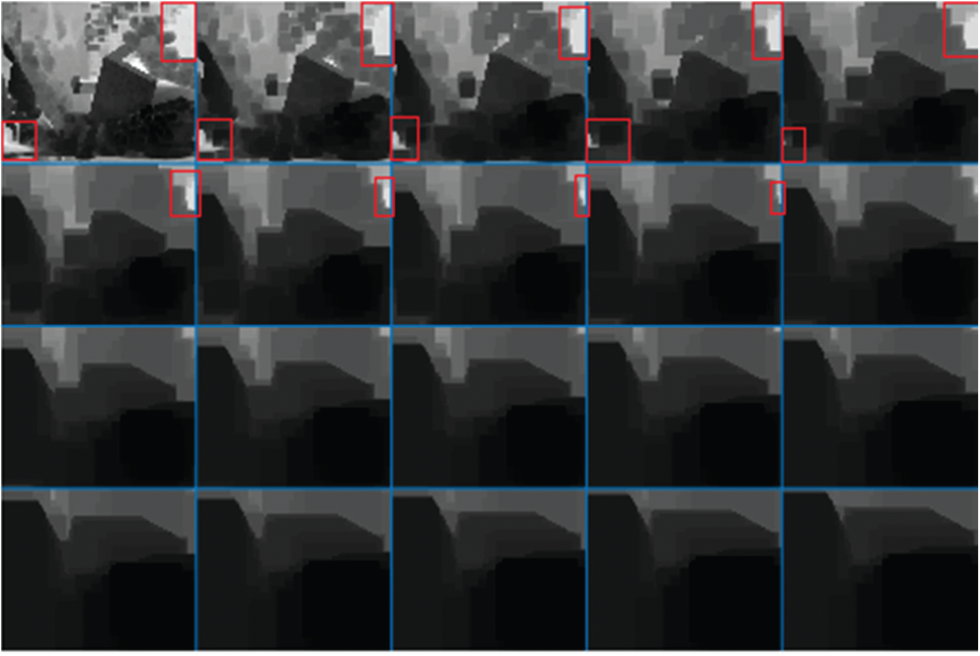
Figure 3: Patch Minimums with different patch sizes
Multiscale patch minimum can be calculated as:
where, N represents the total number of patch minimums and Ω n represents patch size. For multiscale transmission map, the following formulation can followed as:
This will estimate coarse transmission map, which needs to be refined for better edge preservation and less textural noise properties. We use cascaded fast guided filter for edge perversion and textual noise removal.
In proposed algorithm cascaded fast guided filter is used for refinement of coarse transmission map. Firstly it will remove textural noise from coarse transmission map. Secondly the guided filter improves edge perversion properties of estimated transmission map. These textural noise causes halo like artifacts in dehaze image. This issue is addressed in proposed algorithm and smoothing property of fast guided is used to remove extra textural noise. Fig. 4 shows coarse and refines transmission after smoothing and edge preservation properties of fast guided filter.
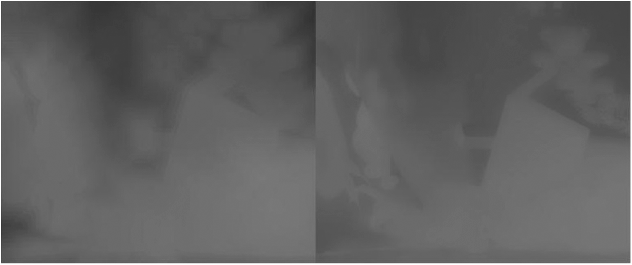
Figure 4: Coarse and refine transmission map. Left to right: Coarse transmission map, refine transmission map (smoothing and edge preservation)
It has been observed that deficiencies in coarse transmission map estimation propagates to refine transmission map and then to dehaze image. In proposed algorithm, we improve transmission map estimation technique and refinement process to achieve optimum transmission map. For Image dehazing rewriting, the formulation is designed as:
To remove low intensity noise in transmission map set a lower limit T of transmission, value should between T ≤ t(x) ≤ 1.
Airlight of hazy image can accurately estimate by using one of these [2,26,27] methods. In experimental comparison constant airlight A is assume for all dehazing algorithms and mentioned at bottom of image. As discussed, performance of dehazing algorithms can estimate by its ability to accurately estimate refine transmission map. Proposed algorithm is compared with baseline DCP [2] and with recent state of art algorithms for diverse and fair results. Results of these algorithms are either taken form author webpage or generated using published source code. The results of Berman et al. [13], Wang et al. [28], Fattal et al. [6], Gibson et al. [29], Kim et al. [30], Nishino et al. [8], Tarel et al. [27] and He et al. [2] are taken from their respective webpages and results of Zhu et al. [16], Lai et al. [31], Yu et al. [1], Meng et al. [7] and He et al. [21] are generated using published source code on author recommended parameters settings. For qualitative comparison standard hazy images are selected from prior dehazing algorithms. Quantitative comparison use standard Middlebury stereo vision [32–35] dataset. The performance of proposed algorithm is also compared using 360p, 480p, 720p, 1080p and 1440p datasets.
Qualitative analysis is visual comparison of dehaze images in term of its visual pleasing, color saturation, visibility and sharpness. Visual analysis of a dehazed image depends on its viewing angle, monitor setting, ambient light and colour preferences of an observer. Hazy images with different scene depths are selected to perceive the performance of proposed algorithm in different conditions. In Figs. 5 and 6, hazy images with distant scene depth are selected to compare their visibility in resultant dehaze images. Proposed algorithm is visually compared with [1,6–8,13,16,17,21]. These algorithms are compared in terms of visibility, clarity of distant object details and colour/contrast saturation.
Fig. 5 shows hazy image of Manhattan city and resultant dehaze images. He et al. [2] shows good colour saturation and clarity but some oversaturated colours can be seen in red marked and sky region. Meng et al. [7] shows unwanted haze and reduced colour saturation especially at red marked region. Fattal et al. [6] shows almost similar results to DCP with better color saturation at sky region. Yu et al. [1], Zhu et al. [16] and Cai et al. [17] shows better color saturation with unwanted haze across resultant image. Berman et al. [13] shows no unwanted haze but over saturated colors can be seen across dehaze image. Proposed algorithms show better results in term of no unwanted haze, no haloes around dark regions and better colour saturation (can be observed in red marked region).
Almost same results can be seen in Fig. 6. It has been observed that Fattals [6] and He et al. [2] algorithms tend to oversaturate some distant hazy objects. Therefore, these regions are marked in red color in Figs. 5 and 6. The comparison of red marked areas can easily show that proposed algorithm can handle depth discontinuities relatively better in terms of clarity, vivid colors and color saturation as compared to [1,6–8,13,16,17,21].
In Figs 7–9 hazy images with relatively close scene depth are selected to observe their visibility, sharpness, haloes and unwanted haze in resultant images. Such images are difficult to dehaze and challenging due to their sharp depth changes as most dehazing algorithms depend on some kind of neighbourhood interpolation scheme [1,6,7,16,26,30]. For these images proposed algorithm is visually compared with [1,6,7,16,21,28,29]. These algorithms are compared in terms of visibility, edge sharpness, unwanted haloes and colour/contrast saturation.
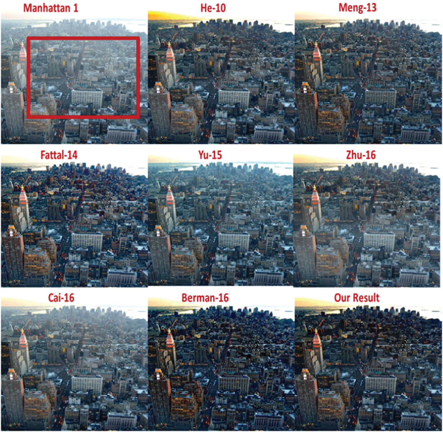
Figure 5: Manhattan image 1 dehazing, A = [0.85, 0.95, 0.99]
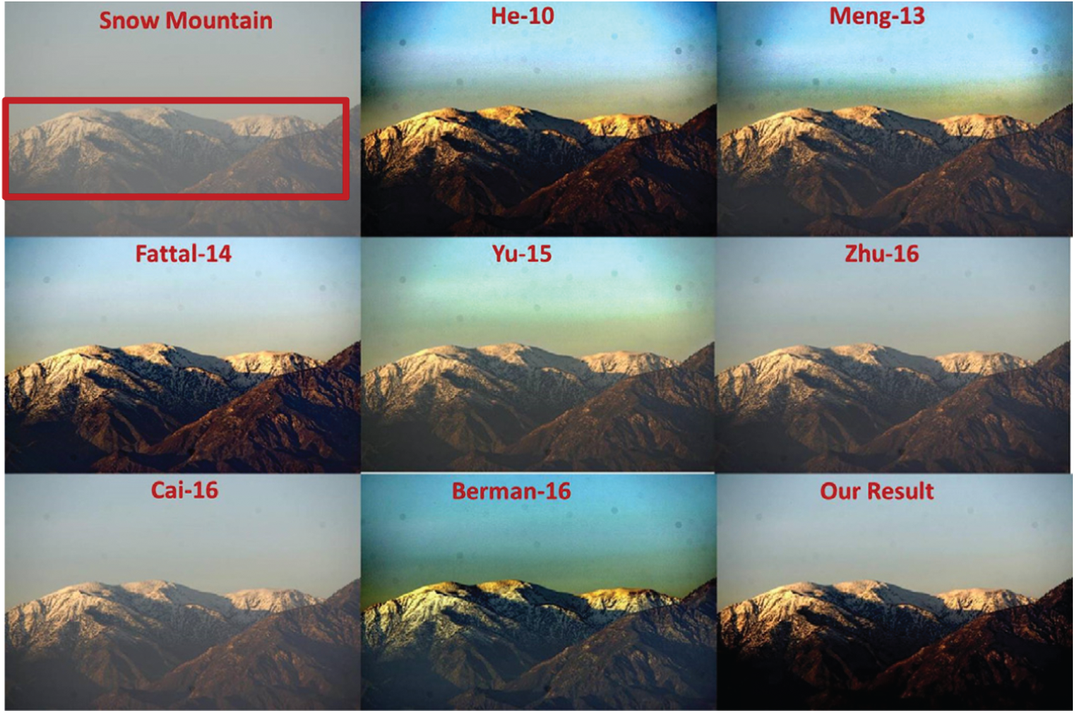
Figure 6: Snow mountain image dehazing, A = [0.67, 0.67, 0.66]
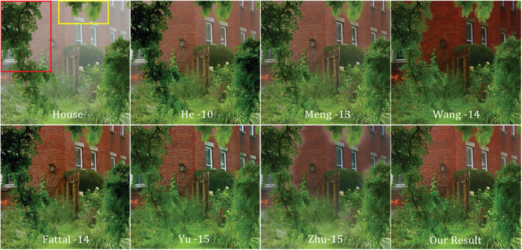
Figure 7: House image dehazing, A = [0.90, 0.97, 0.98]
Hazy image in Fig. 7 is a good test to observe unwanted haloes, sharpness and color saturation of dehazed image. He et al. [2] shows no unwanted haloes but has over saturated colors on tree leaves and small unwanted haze can be seen across the image. Meng et al. [7] shows good color saturation but has less sharpness on tree leaves and small unwanted haze can be observed across the image. Wang et al. [28] shows no unwanted haze but less sharpness on tree leaves and oversaturated unnatural colors can be observed across the image. Fattal et al. [6] shows good color saturation and sharpness but oversaturated colors on tree leaves and haloes around dark regions can be seen at ground region. Yu et al. [1] shows good color saturation but less sharpness and haloes around dark regions can be seen at ground region. Zhu et al. [16] show unwanted haze, strong unwanted haloes and less sharp edges. The proposed algorithm show better results in term of colour saturation, sharpness (can be seen on tree leaves) and no unwanted haloes around dark objects (can be observed in garden region) of dehazed image.
Hazy image in Fig. 8 is a good test to observe sharpness and unwanted haze. He et al. [2] shows good colour saturation, good visibility and no unwanted haloes but it shows has less sharpness on tree leaves can be seen in red marked region. Gibson et al. [29] shows good color saturation but unwanted haze for distant trees and less sharpness on tree leaves can be observed. Fattal et al. [6] shows good color saturation and sharpness but unwanted haze for distant trees can be observed. Yu et al. [1] shows good visibility, sharpness and very little unwanted haze. In comparison proposed algorithms show better results in term of sharpness (can be observed on tree leaves) and least amount of unwanted haze (can be observed at distant trees).

Figure 8: Forrest trees image dehazing, A = [0.82, 0.84, 0.86]
Almost same results can be seen in Fig. 9. By observing each dehaze image very closely and comparing each algorithm. Dehaze images of He et al. [2], Yu et al. [1] and proposed algorithm are selected for further analysis and it has been observed dehaze images of Yu et al. [1] and He et al. [2] tend to loose edge sharpness and oversaturate distant hazy objects, these regions are marked in red and yellow color in Figs. 7–9. By comparison these marked regions, it is easily observed proposed algorithm can gracefully handle depth discontinuities, shows better clarity, with more vivid colors and better color saturation as compared to [1–2,6,7,21,28,29,31]
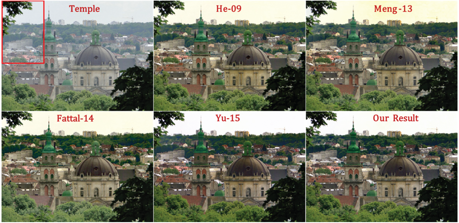
Figure 9: Temple image dehazing, A = [0.73, 0.80, 0.92]
In image processing, quantitative analysis are assumed to be more realistic and accurate approach. Unlike qualitative analysis it do not depend on observer viewing angle, monitor setting, ambient light and colour preferences. A quantitative analysis depends on calculated and statistical results. In this paper, proposed algorithm is quantitative compare with [1,7,13,16,17,21] on a set artificially hazy images using mean square error (MSE) and structure similarity index (SSIM). Dehaze images of each algorithm is compared to their ground truth image to accurately calculate the performance of each dehazing algorithm, as shown in Figs. 10 and 11.
For comparison, ground truth images of Middlebury stereo vision dataset [32–34] and their respective depth maps are used to generate artificial hazy images. A set of five hazy images is generated using Eqs. (1) and (2) assuming β = 0.66. The proposed algorithm is compared with [1,7,13,16,17,26]. Hazy images along with their ground truth and resultant dehaze images are shown in Fig. 12 and DCP shortcoming region are marked in red colour for comparison. Structure similarity index (SSIM) and mean square error (MSE) of dehaze images by each algorithm can be seen in Tab. 1.
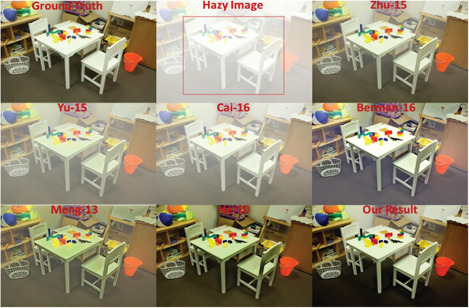
Figure 10: Playroom - Image synthetic dehazing
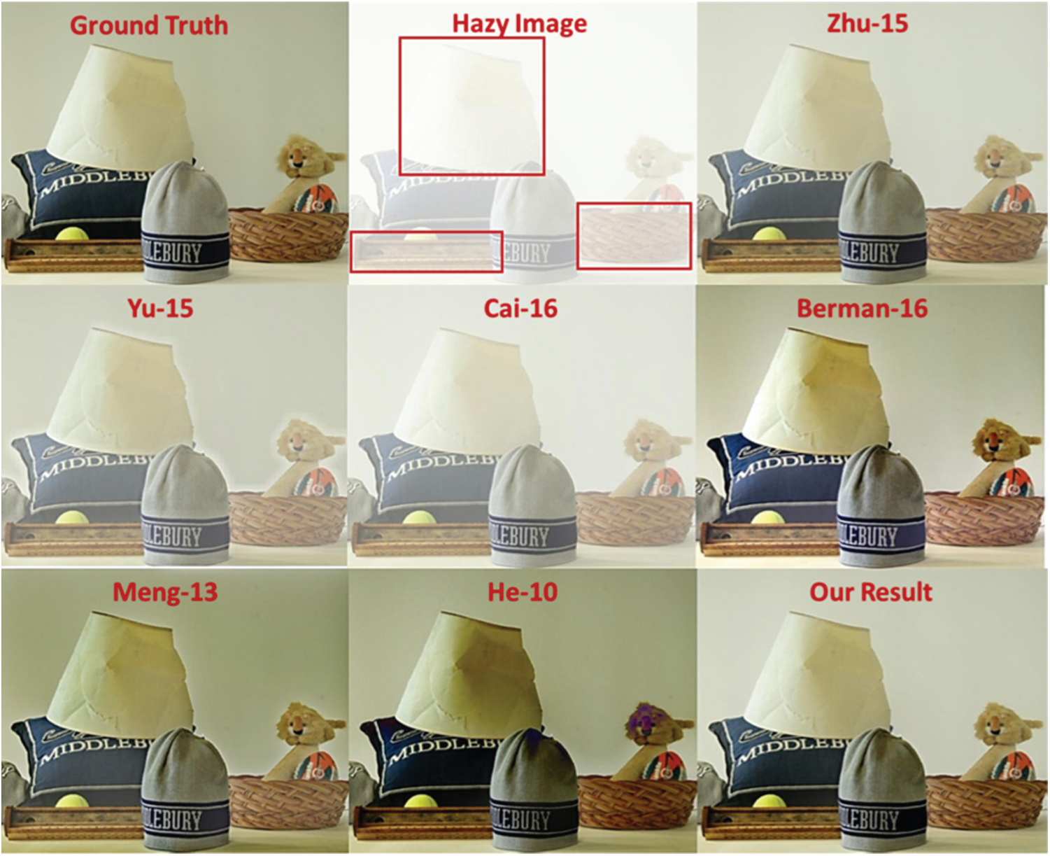
Figure 11: Cap - Image synthetic dehazing
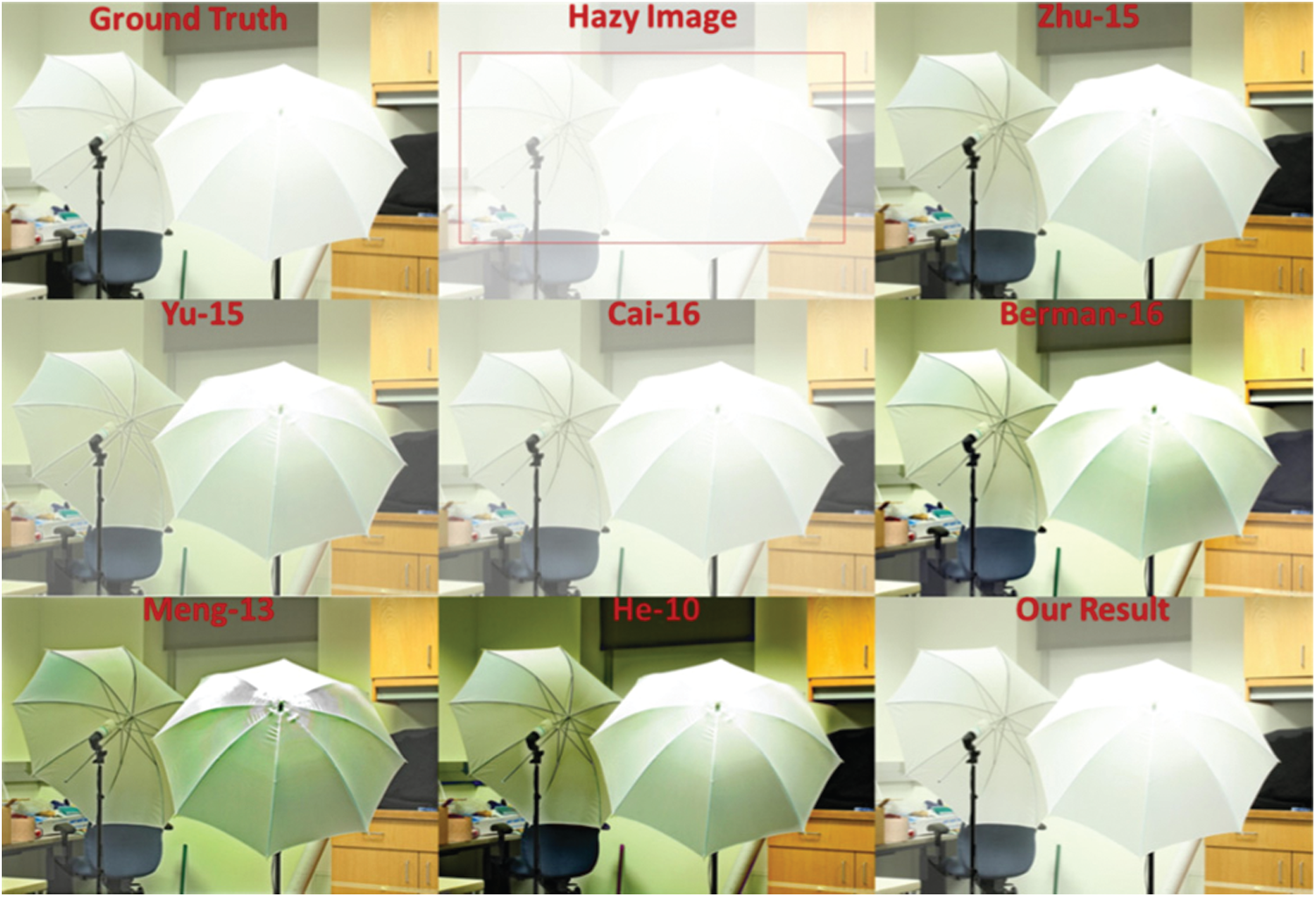
Figure 12: Umbrella - Image synthetic dehazing
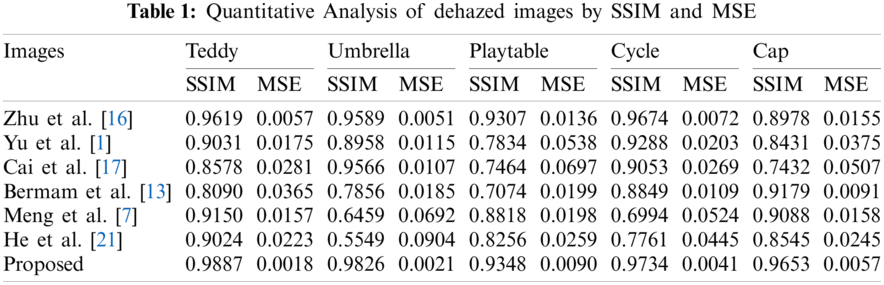
The comparison of the marked regions depicts that the proposed algorithm handles DCP shortcoming (bright surfaces) most gracefully than all reference algorithms. These results are also statistically proven in Tab. 1 by comparing SSIM and MSE of proposed algorithm with prior dehazing algorithms.
Performance analysis is computational speed comparison of different algorithms for same problem. For performance analysis, proposed algorithm is compared with reference dehazing algorithms [1,7,13,16,17,26]. Dataset of 360p (360 x 640), 480p (480 x 854), 720p (720 x 1280), 1080p (1080 x 1920) and 1440p (1440 x 2560) images are used for comparison of each algorithm. Computational time of references algorithms are increasing with resolution image but proposed algorithm use an efficient scaling technique during transmission map estimation which gives an advantage of very low degradation in performance with increasing image resolution. Both scaling and without scaling results of proposed algorithm is shown in Tab. 2 to show high performance improvement of proposed algorithm by adding this efficient scaling technique.
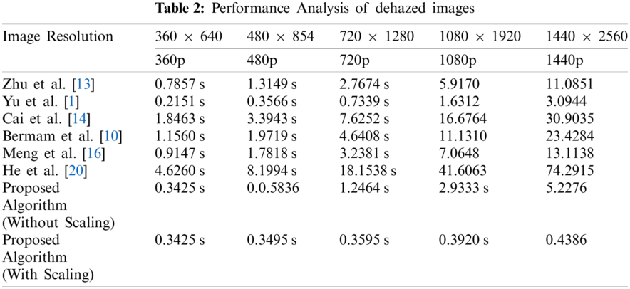
Proposed algorithm sample down every haze image to constant 360p (360 x 640) resolution to estimates its transmission map. This gives an advantage of almost constant computational speed for increasing image resolution. Similarly, Yu et al. [1] uses a minimum filter to sample down hazy image then use block to pixel interpolation scheme for transmission map refinement which quiet fast technique for low resolution images but for high resolution images size of down sampled image is also increases and performance is also degrade massive due to evolution of nine Gaussian terms per pixels.
The results are generated in Matlab® 2017 running on 2.2 GHz Intel i7 processor and summarized in Tab. 2. These results show proposed algorithm significantly improves computational time for both low and high resolution images and is about 11x–280x more faster than guided filter DCP [21]. about 2x–42x more faster than Colour attenuation [16], about 0x–13x more faster than Block-to-pixel-interpolation [1].
An innovative method for image dehazing is implemented that encourages an efficient and halo free image dehazing. By overviewing of different dehazing techniques it is shown that despite remarkable improvements, these algorithms lack in performance in adverse circumstances.Being state of art algorithm Dark channel prior (DCP) is still not utilized to its full potential, which creates room of improvement. We propose an efficient single image dehazing algorithm with improved bright-surface handling capabilities. Proposed algorithm outperforms reference algorithms in terms of speed, quality and handling bright surfaces. Results are compared with reference algorithm through qualitative, quantitative and computational time.
Funding Statement: This research was supported by the MSIT (Ministry of Science and ICT), Korea, under the ICAN (ICT Challenge and Advanced Network of HRD) program (IITP-2021-2020-0-01832) supervised by the IITP (Institute of Information & Communications Technology Planning & Evaluation) and the Soonchunhyang University Research Fund.
Conflicts of Interest: The authors declare that they have no conflicts of interest to report regarding the present study.
1. Y. Teng, I. Riaz, P. Jingchun and S. Hyunchul, “Real-time single image dehazing using block-to-pixel interpolation and adaptive dark channel prior,” IET Image Processing, vol. 9, pp. 725–734, 2015. [Google Scholar]
2. K. He, J. Sun and X. Tang, “Single image haze removal using dark channel prior,” IEEE Transactions on Pattern Analysis and Machine Intelligence, vol. 33, pp. 2341–2353, 2011. [Google Scholar]
3. R. Fattal, “Single image dehazing,” Acm Transactions on Graphics, vol. 27, pp. 1–9, 2008. [Google Scholar]
4. S. G. Narasimhan and S. K. Nayar, “Contrast restoration of weather degraded images,” IEEE Transactions on Pattern Analysis and Machine Intelligence, vol. 25, pp. 713–724, 2003. [Google Scholar]
5. S. G. Narasimhan and S. K. Nayar, “Chromatic framework for vision in bad weather,” in Proc. IEEE Conf. on Computer Vision and Pattern Recognition, NY, USA, pp. 598–605, 2000. [Google Scholar]
6. R. Fattal, “Dehazing using color-lines,” Acm Transactions on Graphics, vol. 34, pp. 1–14, 2014. [Google Scholar]
7. J. Kopf, B. Neubert, B. Chen, M. Cohen, D. Cohen-Or et al., “Deep photo: Model-based photograph enhancement and viewing,” Acm Transactions on Graphics, vol. 27, pp. 1–10, 2008. [Google Scholar]
8. S. G. Narasimhan and S. K. Nayar, “Interactive (de) weathering of an image using physical models,” in IEEE Workshop on Color and Photometric Methods in Computer Vision, NY, USA, p. 1, 2003. [Google Scholar]
9. Y. Y. Schechner, S. G. Narasimhan and S. K. Nayar, “Instant dehazing of images using polarization,” in Proc. IEEE Conf. on Computer Vision and Pattern Recognition, NY, USA, pp. 325–332, 2001. [Google Scholar]
10. D. Berman, T. Treibitz and S. Avidan, “Non-local image dehazing,” in 2016 IEEE Conf. on Computer Vision and Pattern Recognition, LAS VEGAS, USA, pp. 1674–1682, 2016. [Google Scholar]
11. K. Tang, J. Yang and J. Wang, “Investigating haze-relevant features in a learning framework for image dehazing,” in 2014 IEEE Conf. on Computer Vision and Pattern Recognition, LAS VEGAS, USA, pp. 2995–3002, 2014. [Google Scholar]
12. L. Breiman, “Random forests,” Machine Learning, vol. 45, pp. 5–32, 2001. [Google Scholar]
13. Z. Qingsong, M. Jiaming and S. Ling, “A fast single image haze removal algorithm using color attenuation prior,” IEEE Transaction on Image Processing, vol. 24, pp. 3522–3533, 2015. [Google Scholar]
14. B. Cai, X. Xu, K. Jia, C. Qing and D. Tao, “Dehazenet: An end-to-end system for single image haze removal,” IEEE Transactions on Image Processing, vol. 25, pp. 5187–5198, 2016. [Google Scholar]
15. G. Meng, Y. Wang, J. Duan, S. Xiang and C. Pan, “Efficient image dehazing with boundary constraint and contextual regularization,” in 2013 IEEE Int. Conf. on Computer Vision, Sakaka, SA, pp. 617–624, 2013. [Google Scholar]
16. K. Nishino, L. Kratz and S. Lombardi, “Bayesian defogging,” International Journal of Computer Vision, vol. 98, pp. 263–278, 2012. [Google Scholar]
17. P. S. Chavez, “An improved dark-object subtraction technique for atmospheric scattering correction of multispectral data,” Remote Sensing of Environment, vol. 24, pp. 459–479, 1988. [Google Scholar]
18. B. Li, S. Wang, J. Zheng and L. Zheng, “Single image haze removal using content-adaptive dark channel and post enhancement,” IET Computer Vision, vol. 8, pp. 131–140, 2014. [Google Scholar]
19. K. B. Gibson and T. Q. Nguyen, “An analysis of single image defogging methods using a color ellipsoid framework,” Eurasip Journal on Image and Video Processing, vol. 2013, pp. 1–14, 2013. [Google Scholar]
20. K. He, J. Sun and X. Tang, “Guided image filtering,” IEEE Transactions on Pattern Analysis and Machine Intelligence, vol. 35, pp. 1–14, 2013. [Google Scholar]
21. K. B. Gibson and T. Q. Nguyen, “On the effectiveness of the dark channel prior for single image dehazing by approximating with minimum volume ellipsoids,” in 2011 IEEE Int. Conf. on Acoustics, Speech and Signal Processing, NY, USA, pp. 1253–1256, 2011. [Google Scholar]
22. K. B. Gibson, D. T. Vo and T. Q. Nguyen, “An investigation of dehazing effects on image and video coding,” IEEE Transactions on Image Processing, vol. 21, pp. 662–673, 2012. [Google Scholar]
23. E. Matlin and P. Milanfar, “Removal of haze and noise from a single image,” ACM Transactions on Graphics, vol. 8296, pp. 1–8, 2012. [Google Scholar]
24. A. Levin, D. Lischinski and Y. Weiss, “A closed-form solution to natural image matting,” IEEE Transaction Pattern Analysis and Machine Intelligence, vol. 30, pp. 228–42, 2008. [Google Scholar]
25. H. Kaiming, S. Jian and T. Xiaoou. “Guided image filtering,” IET Image Processing, vol. 7, pp. 1–13, 2014. [Google Scholar]
26. J. P. Tarel and N. Hautiere, “Fast visibility restoration from a single color or gray level image,” in 2009 IEEE 12th Int. Conf. on Computer Vision, NY, USA, pp. 2201–2208, 2009. [Google Scholar]
27. Y. K. Wang and C. T. Fan, “Single image defogging by multiscale depth fusion,” IEEE Transaction on Image Processing, vol. 23, pp. 4826–37, 2014. [Google Scholar]
28. K. B. Gibson and T. Q. Nguyen, “Fast single image fog removal using the adaptive wiener filter,” in 2013 IEEE Int. Conf. on Image Processing, NY, USA, pp. 714–718, 2013. [Google Scholar]
29. J. -H. Kim, W. -D. Jang, J. -Y. Sim and C. -S. Kim, “Optimized contrast enhancement for real-time image and video dehazing,” Journal of Visual Communication and Image Representation, vol. 24, pp. 410–425, 2013. [Google Scholar]
30. Y. H. Lai, Y. L. Chen, C. J. Chiou and C. T. Hsu, “Single-image dehazing via optimal transmission map under scene priors,” IEEE Transactions on Circuits and Systems for Video Technology, vol. 25, pp. 1–14, 2015. [Google Scholar]
31. D. Scharstein and C. Pal, “Learning conditional random fields for stereo,” in 2007 IEEE Conf. on Computer Vision and Pattern Recognition, LAS VEGAS, USA, pp. 1–8, 2007. [Google Scholar]
32. H. Hirschmuller and D. Scharstein, “Evaluation of cost functions for stereo matching,” in 2007 IEEE Conf. on Computer Vision and Pattern Recognition, NY, USA, pp. 1–8, 2007. [Google Scholar]
33. D. Scharstein and R. Szeliski, “High-accuracy stereo depth maps using structured light,” in 2003 IEEE Computer Society Conf. on Computer Vision and Pattern Recognition, NY, USA, pp. 1.10, 2011. [Google Scholar]
34. D. Scharstein and R. Szeliski, “A taxonomy and evaluation of dense two-frame stereo correspondence algorithms,” International Journal of Computer Vision, vol. 47, pp. 7–42, 2002. [Google Scholar]
35. D. Scharstein and R. Szeliski, “A taxonomy and evaluation of dense two-frame stereo correspondence algorithms,” International Journal of Computer Vision, vol. 47, pp. 7–42, 2002. [Google Scholar]
 | This work is licensed under a Creative Commons Attribution 4.0 International License, which permits unrestricted use, distribution, and reproduction in any medium, provided the original work is properly cited. |