Computers, Materials & Continua DOI:10.32604/cmc.2022.016152
Article

Tour Planning Design for Mobile Robots Using Pruned Adaptive Resonance Theory Networks

S. Palani Murugan1,*, M. Chinnadurai1 and S. Manikandan2

1Department of CSE, E. G. S. Pillay Engineering College, Nagapattinam, 611002, Tamil Nadu, India
2Department of IT, E. G. S. Pillay Engineering College, Nagapattinam, 611002, Tamil Nadu, India
*Corresponding Author: S. Palani Murugan. Email: suyambhu11@gmail.com
Received: 08 April 2021; Accepted: 10 May 2021

Abstract: The development of intelligent algorithms for controlling autonom- ous mobile robots in real-time activities has increased dramatically in recent years. However, conventional intelligent algorithms currently fail to accurately predict unexpected obstacles involved in tour paths and thereby suffer from inefficient tour trajectories. The present study addresses these issues by proposing a potential field integrated pruned adaptive resonance theory (PPART) neural network for effectively managing the touring process of autonomous mobile robots in real-time. The proposed system is implemented using the AlphaBot platform, and the performance of the system is evaluated according to the obstacle prediction accuracy, path detection accuracy, time-lapse, tour length, and the overall accuracy of the system. The proposed system provide a very high obstacle prediction accuracy of 99.61%. Accordingly, the proposed tour planning design effectively predicts unexpected obstacles in the environment and thereby increases the overall efficiency of tour navigation.

Keywords: Autonomous mobile robots; path exploration; navigation; tour planning; tour process; potential filed integrated pruned ART networks; AlphaBot platform

1  Introduction

Fixed robotics have been widely applied for many years in numerous settings where environmental conditions are known with a very high degree of certainty. However, mobile robots have the capacity to perform a much wider range of activities, such as explore terrestrial, underwater, aerial, and outer space environments, transport cargo, complete complex tasks, perform surgery, assist in warehouse distribution centers, support security, act as a personal assistants, aid in space and ocean exploration, and provide guidance for navigation [1–4]. Mobile robots that implement well-defined tasks in highly controlled environments rely upon preprogrammed or externally communicated instructions and guidance rules for moving about the environment, and generally implement only simplistic obstacle avoidance algorithms. In contrast, the goal of autonomous mobile robots is to implement tasks within uncontrolled environments without any external direction. Accordingly, autonomous mobile robots must maneuver around obstacles, in addition to addressing all other issues that guided mobile robots encounter [5]. These features are achieved by mobile robots using several technologies, such as various sensors, wireless communication, integrated safety, fleet simulation software, supervisory software, and fleet management software [6]. The first electronic autonomous mobile robots were Elmer and Elsie, which were created by Dr. William Grey Walter in 1948 in Bristol, England [7]. This and subsequent developments in autonomous mobile robot design relied upon conventional obstacle avoidance algorithms. However, efficient autonomous operation requires predictive capabilities based upon feedback from the environment, which cannot be obtained via conventional algorithms. The first autonomous mobile robot to be controlled with the help of artificial intelligence was introduced in 1970 [8].

More recent efforts to improve the predictive capabilities of autonomous mobile robots have been based upon the development of increasingly sophisticated artificial neural networks (ANNs) [9]. For example, Tai et al. [10] implemented an ANN by integrating a convolutional neural network(CNN)with the respective decision-making process to facilitate effective robot exploration based on visual cues. The autonomous mobile robot system was trained using annotated visual information related to the exploration task, and its efficiency was evaluated in a real-time application. Similarly, Thomas et al. [11] applied a CNN in the FumeBot home monitoring robot system. Obstacles in the home environment were effectively identified from image data during the training process. Bing et al. [12] developed effective autonomous mobile robot control for exploration applications using a spiking neural network (SNN)in conjunction with various robot characteristics, such as energy, speed, and computational capabilities, during network training. The efficiency of the system was evaluated via simulations. Patnaik et al. [13] developed autonomous mobile robot control using an evolving sensory data-based network approach. Four different learning models were applied during network training to predict both obstacles and targets in the surrounding environment based on their sizes and shapes.

The present work addresses these issues by proposing a potential field integrated pruned adaptive resonance theory (PPART) neural network for effectively managing the touring process of autonomous mobile robots in real-time based on a very high accuracy for predicting unexpected obstacles in the environment. The excellent obstacle prediction accuracy then facilitates the development of highly efficient robot trajectories in real time. Specifically, the potential field method is employed to conduct path exploration according to a given destination and the presence of obstacles in the path exploration space based on the Laplace equation and an energy field representation of the path exploration space, including the destination and obstacles within that space. The adaptive resonance theory (ART) neural network is then employed in conjunction with the determined obstacles to obtain the optimal navigation path that avoids all obstacles and is the shortest possible path to achieve operational objectives. Here, the optimal navigation pathways are identified by fuzzy and ART neural networks based on building maps that consist of several geometric primitives. The remainder of this manuscript is organized as follows. Section 2 presents the PPART neural network in detail. The obstacle prediction and path detection performance, and the tour efficiency obtained by the network are evaluated in Section 3. Finally, Section 4 concludes the manuscript.

2  Potential Field Integrated Pruned Adaptive Resonance Theory Neural Network

Assumptions and Notations

The following assumptions and notations are applied to identify the obstacles, ideal travel paths, and navigation process of an autonomous mobile robot [14].

•   The tour planning working environment with in which the mobile robot is placed is defined as WE, and the boundary of the environment is denoted as the tour environment boundary (TEB).

•   A specific area to be analyzed and accessed by the robot in WE is denoted as WEa, which is approximately a circle with a radius defined as ra.

•   The WE and TEB contain both unknown and known stationary obstacles with unknown positions and shapes.

•   The shape of the mobile robot is approximately a circle with a radius defined as Rrobot.

•   The mobile robot path configuration space in WE is defined as SP, and the free space is defined as SPfree.

•   The robot sensing data captured with in WEa is defined as RSsensing, and the specific area radius is defined as ra.

Mobile Robot Path Identification Process Based on the Potential Field

The path exploration problem and any obstacles within the defined environment WEmust be identified [15]. Initially, the obstacles are identified through RSsensing are, and the points are connected to facilitate path exploration in WE. The primary objective of the path identification process is to minimize the path length by analyzing all of the obstacles present in WE. To this end, we first define the respective observation points of the mobile robot as pii (i=1,2,…,N), where N is the total number of observation points. The defined observation points must satisfy the following equation:

∀pis∈WEa,∃i∈{1,2,…,N},‖pis−pii‖≤ri(1)

Once the observation points related to the path exploration process are detected, the detected robot path must adhere to the mapping relation pi(t):[0,1]→WEa. Therefore, the following condition must also be satisfied:

pi(0)=Pi(1)=piτ1,(2)

pi(i−1N)=piτi(i=2,3…,N),(3)

where τi is defined as the path navigation of all observation points pii… During exploration, the path initiates from p(0) and traverses to the initial point p(1). The tour planning process and the kinematic robot model are illustrated in Fig. 1. The motion of the mobile robot in the defined system is constrained in WE using the following dynamic non-holonomic constraints in the x, y, and z translational directions and in the rotational direction [16]:

x˙=z.cos(φ)(4)

z=(ZR+ZL)2(5)

y˙=m.sin⁡(φ),(6)

m=(ZR−ZL)L(7)

where z is the translational velocity of the robot, the angular robot orientation is represented as φ, ZR represents the translational velocity of the right wheel, ZL denotes the translational velocity of the left wheel, m denotes the robot's rotational velocity, and L is the distance between the right and left wheels [17].

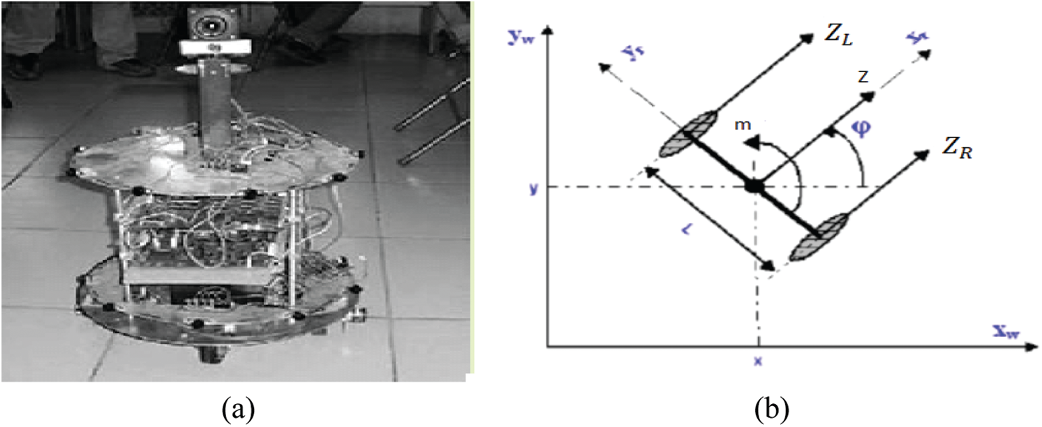
Figure 1: (a) Sample mobile robot and (b) Kinematic robot model

During the analysis process, WE is split into grids within which the obstacles and destination are represented, and the obstacles and destination are respectively assigned repulsive and attractive potentials according to an artificial potential field [18]. This converts robot path exploration into an energy minimization problem [19]. A representative potential field within a divided working space is illustrated in Fig. 2, where the green color represents the attractive potential of the destination and the brown color represents the repulsive potential of the obstacles. The potentials presented in Fig. 2 are defined in the following discussion.

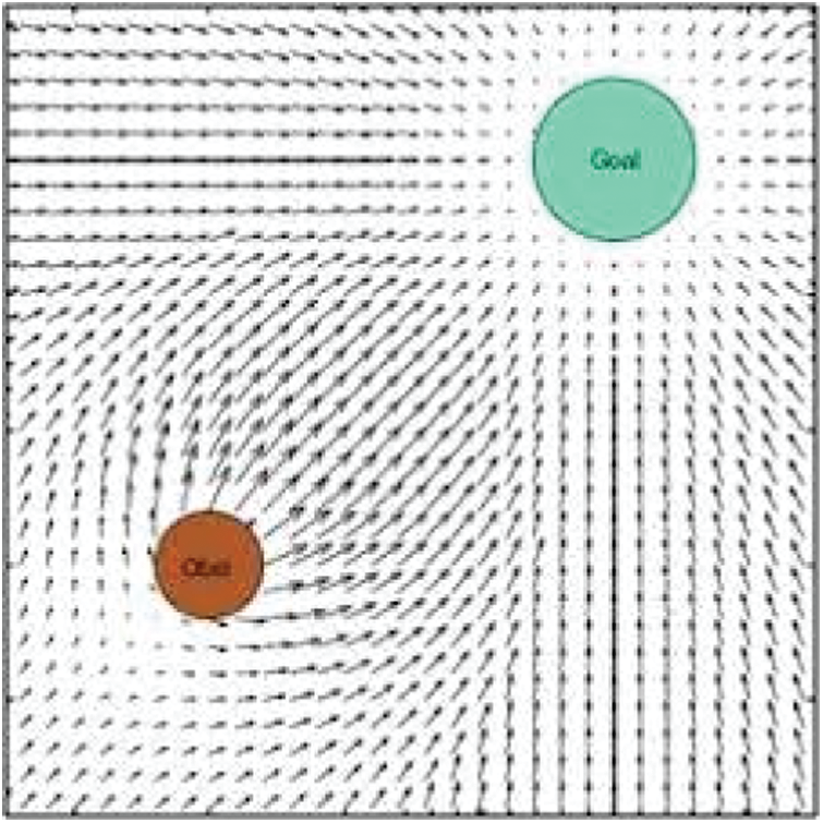
Figure 2: Working environment representation using potential field

The attractive potential of the destination is defined as follows:

Pg=c|x−xgoal|2+|y−ygoal|2(8)

where x and y are the robot coordinates in two-dimensional (2D) space, xgoal and ygoal are the 2D coordinates of the destination, and c is a constant. Then, the potentials of obstacles in WE are defined as follows:

pi,j=pmax1+g(9)

where pmax is the maximum potential ofWE, and g is derived as follows.

g(x,y)=(x0−l2−x)+|x0−l2−x|+(x−x0−l2+1)+|x−x0−l2+1|+(y0−l2−y)+|y0−l2−y|+(y−y0−l2+1)+|y−y0−l2+1|.(10)

Here, xo and yo are the 2D coordinates of the obstacle, and l is the obstacle length. In addition, robot path exploration is maintained within WE by applying a repulsive potential to the TEB as follows:

PHA=1δ+∑i=1s⁡(gi+|gi|)(11)

Here, δ is a constant, gi is a linear boundary convex region function, and the boundary face segments are represented as s. Finally, the total potential acting on the robot at (x, y) is computed as the sum of the attractive and repulsive potentials:

Utotal=Pg+Po+PHA(12)

The successful identification of WE,RSsensing, and ∀pis∈WEa,∋i∈{1,2,…,N},‖pis−pii‖≤ri are used to define the obstacle-related information in WE. These observation points are analyzed by the kinematic constraints of the mobile robot, such as x¨ and y¨ The positions of all obstacles in WE are then predicted based on an effective examination of the values of Po.

The output of this process generates vector information I = [I1I2…IM]T of length M, where each element lies in a range (0, 1), which, along with the geometric primitives and corresponding parameters, is represented as velocity, position, and acceleration into the ART neural network.

Mobile Robot Navigation Using an ART Neural Network

The proposed ART neural network architecture and corresponding processing are illustrated in Fig. 3. The network consists of an input layer denoted as F0. that receives vector inputs I = [I1I2…IM]T. The incoming inputs are received as y1 = [y11y12…y1M]T by the following layer F1 in the bottom-up process, which are then transmitted to the following layer F2 as y2 = [y21y22…y2N]T of length N in the top-down inputs, where the inputs I are processed. After initializing the input vectors and respective processing layers, the particular weight values of the network nodes are denoted as wj = {wj1, wj2,…, wjM}.

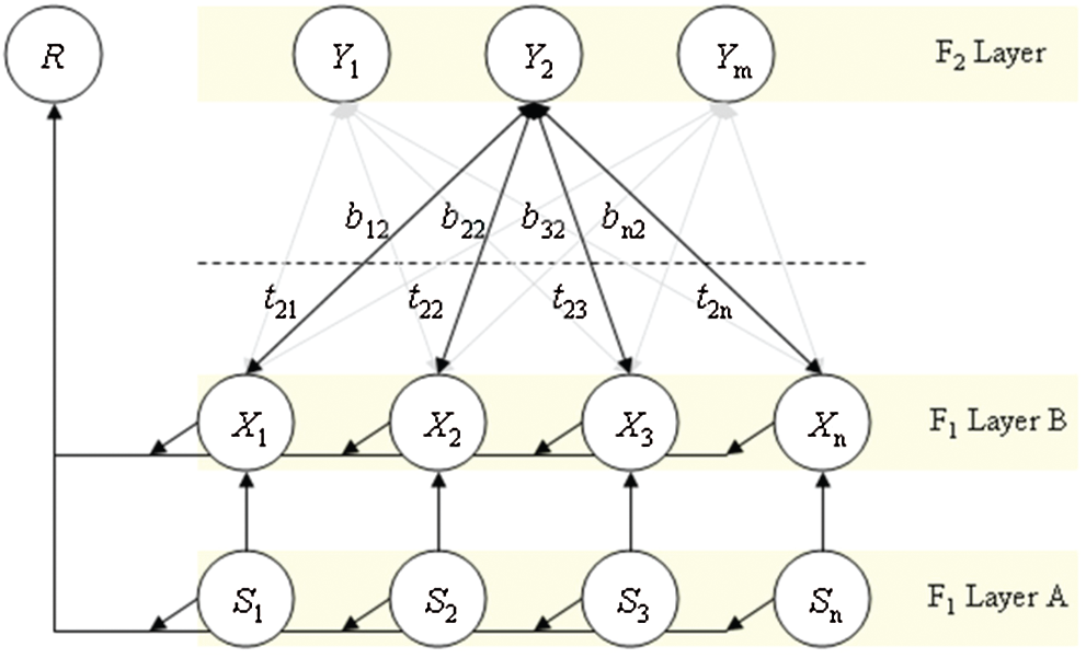
Figure 3: ART network structure

The specific navigation choice function is defined as follows:

Tj(I)=|I∧wj|(α+|wj|).(13)

Here, ∧ represents the fuzzy operator defined as

(p∧q)i=min(pi,qi)(14)

where pi and qi denote M-dimensional vectors. In addition, α is the scalar value, and the Manhattan norm is applied, which is estimated as follows:

|p|=∑i=1M⁡|pi|(15)

Furthermore, a matching process is performed for every incoming input, where upon the exact navigation path is identified successfully. Otherwise, network training is continued by updating the weight values as follows:

wJnew=β(I∧wJold)+(1−β)wJold(16)

Here, the ART network uses the learning parameter β is 1 and vigilance parameter ρ to implement a very fast network training process. The value of β lies in the range (0, 1), and a constant value of ρ is employed.

The complete training process is illustrated in Fig. 4. Here, category pruning, direct category updating, and direct category creation are applied to further refine the ART network output.

In the category pruning process, a fuzzy ART rectangular map is identified for every obstacle present in WE. The pruning process removes obstacles related to the rectangular map from the touring environment, and the related categories are also eliminated from the list. The weight values of the removed obstacles are written in the form of wj=(uj,vjc), where uj and vjc are the vertices of the corresponding rectangular map. Finally, the respective weight values are changed in both layers F1 and F2. For layer F1, these are computed as follows.

{y1j:=y1Ny2j:=y2Nwij:=wNi,i=1,2,…,M.(17)

For layer F2, the weight values are computed as follows.

{N:=N−1wN−1=…=wNM=1(18)

This process is repeated for all removed obstacles in the touring environment.

Figure 4: Pruned ART network learning process

Then, direct category updating is applied to the ART network to resize the rectangular map categories. In addition, the corresponding weight values are also updated as wj=(uj,vjc) according to the new vertices of the rectangular maps. This process is repeated whenever the size of a rectangle map decreases or one map divides into two or more maps.

Finally, direct category creation is applied whenever the incoming input is not matched with the trained features. Moreover, categories are created only when obstacles are present in the environment. A new rectangular map is created with the respective weight values defined above, and a new category is created (Eq. (19)). Afterward, the category value is increased continuously to meet the corresponding tour path.

{N=N+1wN1=…=wNM=0(19)

According to the above discussion, each incoming input feature is processed by a pruned ART network that completely recognizes the obstacles present in the environment. Then, the effective navigation path is detected from source to destination by eliminating unwanted categories from the list. This process is repeated, and the mobile robot efficiently moves in the tour environment until reaching the destination.

3  Experimental Analysis

The proposed PPART approach was developed using the AlphaBot robotic development platform. The development platform is compatible with Ardunio and Raspberry Pi, and includes several components, such as a mobile chassis and a main control board for providing motion within a test environment boundary. The effective utilization of the components and compatibility helps to predict the obstacles, line tracking, infrared remote control, Bluetooth, ZigBee process, and video monitoring. The mobile robot path exploration and navigation process performance provided by the PPART neural network is evaluated according to its obstacle prediction accuracy, path detection accuracy, error rate, and overall system accuracy based on different evaluation metrics. The accuracy of obstacle prediction was compared with those obtained using three existing machine learning techniques, including ANN-,CNN-, and SNN-based methods.

Tab. 1 lists the average obstacle prediction accuracy obtained by the four methods considered based on 250 touring attempts. The results in the table demonstrate that the obstacle prediction accuracy of the PPART approach effectively predicts the artificial potential regions in WE. This prediction process is facilitated by the continuous collection of observation points in WE. The results in Tab. 1 are graphically presented in Fig. 5 for a more intuitive appraisal of the obstacle prediction accuracy of the proposed approach.

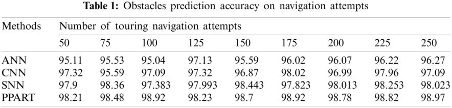
Figure 5: Obstacles detection accuracy on the number of navigation attempts

In addition, the efficiency of the obstacle detection process was analyzed, the results of which are listed in Tab. 2. The results in the table clearly demonstrate that the proposed PPART approach efficiently predicts the obstacles present in WE. The results in Tab. 2 are graphically presented in Fig. 6.

Figure 6: Obstacles detection accuracy based on the time interval

Figs. 5 and 6 illustrate the accuracy and efficiency of obstacle identification. The computation of Pg based on Eq. (8) and PHAbased on Eq. (11) reduce the occurrence of mobile robot navigation outside of the TEB. Meanwhile, the computation of Po based on Eq. (9) maximizes the obstacle detection process. Following the computation of the repulsive potential values, the obstacles are effectively predicted in the different time intervals.

The path navigation accuracy values are listed in Tab. 3. From the table we can understand that the proposed PART approach offers better prediction accuracy in different navigation attempts. The results in Tab. 3 are graphically presented in Fig. 7.

Figure 7: Navigation path accuracy

The efficiency of the navigation path identification process was analyzed. The results, listed in Tab. 4, show that the proposed PART approach offers better prediction accuracy at various time intervals. The results in Tab. 4 are graphically presented in Fig. 8.

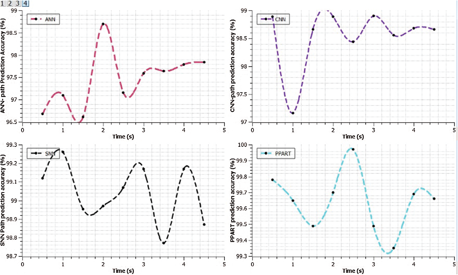
Figure 8: Navigation path prediction accuracy based on time interval

The error rates of the three different classifiers considered in comparison with that of the PPART approach are illustrated in Fig. 9. The overall accuracy obtained by the four classifiers is illustrated in Fig. 10. This figure demonstrates that the PPART approach provides an overall accuracy of up to 99.61%.

Figure 9: Error rate

Figure 10: Accuracy

4  Conclusion

The present work addressed the generally inefficient tour trajectories obtained by conventional intelligent algorithms due to the poor prediction of unexpected obstacles in the environment by proposing the PPART neural network. The potential field method was employed to conduct path exploration according to a given destination and the presence of obstacles in the path exploration space based on an energy field representation of the path exploration space. An ART neural network was then employed in conjunction with the determined obstacles to obtain the optimal navigation path that avoids all obstacles and is the shortest possible path to achieve operational objectives. The proposed system was implemented using the AlphaBot platform, and the performance of the system was evaluated according to the obstacle prediction accuracy, path detection accuracy, and the overall accuracy of the system. These results demonstrated that the proposed system provides a very high obstacle prediction accuracy of 99.61%. Accordingly, the proposed tour planning design effectively predicts unexpected obstacles in the environment, and thereby increases the overall efficiency of tour navigation. In future work, we will seek to improve the efficiency of the mobile robot navigation process by applying optimized techniques.

Acknowledgement: We thank LetPub (https://www.letpub.com) for its linguistic assistance during the preparation of this manuscript.

Funding Statement: The authors received no specific funding for this study.

Conflicts of Interest: The authors declare that they have no conflicts of interest to report regarding the present study.

References

 1.  J. R. G. Sanchez, R. S. Ortigoza, S. T. Mosqueda, G. M. Sanchez, V. M. H. Guzman et al., “Tracking control for mobile robots considering the dynamics of all their subsystems: Experimental implementation,” Complexity, vol. 2017, no. 5318504, pp. 1–18, 2017. [Google Scholar]

 2.  Q. Zhu, Y. Han, P. Liu, Y. Xiao, P. Lu et al., “Motion planning of autonomous mobile robot using recurrent fuzzy neural network trained by extended kalman filter,” Computational Intelligence and Neuroscience, vol. 2019, no. 1934575, pp. 1–16, 2019. [Google Scholar]

 3.  S. Mitsch, K. Ghorbal, D. Vogelbacher and A. Platzer, “Formal verification of obstacle avoidance and navigation of ground robots,” International Journal of Robotics Research, vol. 36, no. 12, pp. 1312–1340, 2017. [Google Scholar]

 4.  D. W. Kim, T. A. Lasky and S. A. Velinsky, “Autonomous multi-mobile robot system: Simulation and implementation using fuzzy logic,” International Journal of Control, Automation and Systems, vol. 11, no. 3, pp. 545–554, 2013. [Google Scholar]

 5.  W. Budiharto, A. Jazidie and D. Purwanto, “Indoor navigation using adaptive neuro fuzzy controller for servant robot,” in Proc. 2010 Second Int. Conf. on Computer Engineering and Applications, Bali Island, pp. 582–586, 2010. [Google Scholar]

 6.  N. A. Vien, N. H. Viet, S. Lee and T. Chung, “Obstacle avoidance path planning for mobile robot based on ant-q reinforcement learning algorithm,” in Proc. Int. Sym. on Neural Networks: Advances in Neural Networks, Berlin, Heidelberg, pp. 704–713, 2007. [Google Scholar]

 7.  A. Aouf, L. Boussaid and A. Sakly, “Same fuzzy logic controller for two-wheeled mobile robot navigation in strange environments,” Journal of Robotics, vol. 2019, no. 2465219, pp. 1–11, 2019. [Google Scholar]

 8.  A. M. Zou, Z. G. Hou, S. Y. Fu and M. Tan, “Neural networks for mobile robot navigation: A survey,” in Proc. Int. Sym. on Neural Networks: Advances in Neural Networks, Berlin, Heidelberg, pp. 1218–1226, 2006. [Google Scholar]

 9.  L. Tai, L. Shaohua and M. Liu, “Autonomous exploration of mobile robots through deep neural networks,” International Journal of Advanced Robotic Systems, vol. 14, no. 4, pp. 1–9, 2017. [Google Scholar]

10. A. Thomas and J. Hedley, “Fumebot: A deep convolutional neural network controlled robot,” Robotics, vol. 8, no. 3, pp. 50–62, 2019. [Google Scholar]

11. Z. Bing, C. Meschede, F. Rohrbein, K. Huang and A. C. Knoll, “A survey of robotics control based on learning-inspired spiking neural networks,” Frontiers in Neurorobotics, vol. 12, no. 35, pp. 1–22, 2018. [Google Scholar]

12. A. Patnaik, K. Khetarpal and L. Behera, “Mobile robot navigation using evolving neural controller in unstructured environments,” IFAC Proc. Volumes, vol. 47, no. 1, pp. 758–765, 2014. [Google Scholar]

13. Y. Quinonez, M. Ramirez, C. Lizarraga, I. Tostado and J. Bekios, “Autonomous robot navigation based on pattern recognition techniques and artificial neural networks,” in Proc. Int. Work-Conf. on the Interplay Between Natural and Artificial Computation (IWINAC 2015Bioinspired Computation in Artificial Systems, Springer, Cham, pp. 320–329, 2015. [Google Scholar]

14. K. B. Reed, A. Majewicz, V. Kallem, R. Alterovitz, K. Goldberg et al., “Robot-assisted needle steering,” IEEE Robotics and Automation Magazine, vol. 18, no. 4, pp. 35–46, 2012. [Google Scholar]

15. R. Solea, A. Filipescu and U. J. Nunes, “Sliding-mode control for trajectory-tracking of a wheeled mobile robot in presence of uncertainties,” in Proc. of 7th Asian Control Conf., Hong Kong, pp. 1701–1706, 2009. [Google Scholar]

16. I. Hassani, I. Maalej and C. Rekik. “Robot path planning with avoiding obstacles in known environment using free segments and turning points algorithm,” Mathematical Problems in Engineering, vol. 2018, no. 2163278, pp. 1–13, 2018. [Google Scholar]

17. H. Seki, S. Shibayama, Y. Kamiyaand M. Hikizu, “Practical obstacle avoidance using potential field for anonholonomic mobile robot with rectangular body,” in Proc. of the 13th IEEE Int. Conf. on Emerging Technologies and Factory Automation, Hamburg, Germany, pp. 326–332, 2008. [Google Scholar]

18. T. Barszcz, A. Bielecki and M. Wojcik, “ART-Type artificial neural networks applications for classification of operational states in wind turbines,” in Proc. Int. Conf. on Artificial Intelligence and Soft Computing, Springer, Berlin, Heidelberg, pp. 11–18, 2010. [Google Scholar]

19. S. Li, D. C. Wunsch, E. O. Hair and M. G. Giesselmann, “Comparative analysis of regression and artificial neural network models for wind turbine power curve estimation,” Journal of Solar Energy Engineering, vol. 123, no. 4, pp. 327–332, 2001. [Google Scholar]

This work is licensed under a Creative Commons Attribution 4.0 International License, which permits unrestricted use, distribution, and reproduction in any medium, provided the original work is properly cited.