DOI:10.32604/cmc.2021.020057
| Computers, Materials & Continua DOI:10.32604/cmc.2021.020057 | |
| Article |
Prediction of the Slope Solute Loss Based on BP Neural Network
1School of Hydrology and Water Resources, Nanjing University of Information Science & Technology, Nanjing, 210044, China
2Water Resources Research Institute, China Institute of Water Resources and Hydropower Research, Beijing, 100044, China
3Department of Geography and Environmental Sustainability, University of Oklahoma, Norman,73071, USA
*Corresponding Author: Xiaona Zhang. Email: nanaxiao86@163.com
Received: 07 May 2021; Accepted: 28 June 2021
Abstract: The existence of soil macropores is a common phenomenon. Due to the existence of soil macropores, the amount of solute loss carried by water is deeply modified, which affects watershed hydrologic response. In this study, a new improved BP (Back Propagation) neural network method, using Levenberg–Marquand training algorithm, was used to analyze the solute loss on slopes taking into account the soil macropores. The rainfall intensity, duration, the slope, the characteristic scale of macropores and the adsorption coefficient of ions, are used as the variables of network input layer. The network middle layer is used as hidden layer, the number of hidden nodes is five, and a tangent transfer function is used as its neurons transfer function. The cumulative solute loss on the slope is used as the variable of network output layer. A linear transfer function is used as its neurons transfer function. Artificial rainfall simulation experiments are conducted in indoor experimental tanks in order to verify this model. The error analysis and the performance comparison between the proposed method and traditional gradient descent method are done. The results show that the convergence rate and the prediction accuracy of the proposed method are obviously higher than that of traditional gradient descent method. In addition, using the experimental data, the influence of soil macropores on slope solute loss has been further confirmed before the simulation.
Keywords: Solute loss; soil macropores; improved BP neural network; slope
The use of soil solute including: soil organic matter, chemical fertilizer, pesticides etc., has been widely accepted as being indispensable in most agricultural systems. The Soil and Fertilizer Institute at the Chinese Academy of Agricultural Sciences, investigated the application amounts of fertilizer and the results showed that the applying of nitrogen is far more than the demand of food crops because only 35% of the fertilizers are absorbed by crops.
One of the main reasons for this may be the existence of soil macropores. A great many indoor and field experimental studies have shown that the existence of soil macropores such as worm holes, root channels and cracks, are common phenomenon. Soil macropores have been recognized as significant pathways for water and solute movement in field soil, although the volume is only 0.1% to 5% of the soil [1,2]. An additional reason may be, that when rainfall intensity exceeds infiltration capacity, an overland flow will be generated which leads to solute migration and loss [3]. In considersing soil macropores, it is meaningful to combine these two reasons when determining the accurate amount of slope solute loss transferring from the soil to the overland flow. This study is not only a basis for regarding nutrient loss, but also is essential for the agricultural management of non-point source pollution [4].
Previous studies have simulated the solute transport process from soil to runoff [5–9]. However, in most of these models, the soil was generally assumed as a homogeneous matterand the soil macropores were ignored.
The importance of the soil macropores for solute transport has been demonstrated, either in situ [10,11] or in the laboratory, by means of breakthrough experiments on small undisturbed soil columns [12,13]. However, recently there has been more concern about: the description of the macropore’s structure; the movement mechanisms of solute in soil macropores, the exchange rules for water and solute movement between the soil matrix region and the macropore region [14–19]. While considering soil macropores, little is yet known about how to determine accurately the amount of slope solute transfer from the soil to the overland flow.
In regards to soil macropores, the solute loss carried by overland flow is a very complex process. There are many parameters influencing this process, such as: rainfall characteristics; land surface characteristics; runoff erosion; soil corrosion resistance; physical and chemical properties of the solute; ambient temperature, and so on [20–23]. The simulation model of the slope solute migration with overland flow, considering soil macropores, should contain all the influence factors, however, each specific aspect of the complex process is still unclear. It is difficult for the existing deterministic model to describe the complex process involved [24].
Based on the measured experimental data, the BP neural network has a strong generalization ability [25–33]. It is not necessary for the BP neural network model to analyze the internal specific process. After the BP neural network model is trained, using the measurement input and output data, the slope solute transport model equivalent to the actual physical process is established. Traditional BP neural network using gradient descent method has a slow convergence rate and is easy to fall into local minimum value. So the objectives of this study are, to try to apply an improved BP neural network prediction method in order to define the process of slope loss transport with overland flow, with consideration to the soil macropores. Also, to test the validity of this method by means of indoor experimentation of artificial rainfall simulation.
The remainer of this study is organized as follows: Section 2, describes the design idea of the improved BP neural network prediction method for slope solute loss considering soil macropores. Section 3 describes the indoor experiment and method in order to verify the validity of the proposed model. The results are presented in Section 4. Section 5 provides a summary of the results and a discussion on the limitations and the practical implications of this study.
2 The Design Idea of the Improved BP Neural Network Prediction Method for Slope Solute Loss Considering Soil Macropores
Based on BP (Back Propagation) error Back Propagation algorithm, BP neural network is multilayer feedforward neural networks. It can learn and store a lot of input-output mapping relation without prior describing the mapping relationship. Traditional BP neural network using gradient descent method has a slow convergence rate and is easy to fall into local minimum value. Therefore, in this paper, the improved BP algorithm is used for solute loss on slope considering soil macropores. In the optimization algorithm, Levenberg–Marquardt algorithm is a very effective method of design optimization. In this method, the error indicator is defined as
where,
The weight adjustment equation is
where,
For the Eq. (1), it is necessary for the matrix of p × p dimensional to inversion calculation. The inverse method of the p × p dimensional matrix is as follows.
If
(3)
Let
At this time, the new weight adjustment equation
For the Eq. (5), it is necessary for solve an inverse of n × n dimension matrix. When the number of network output n = 1,
According to the weights adjustment of Eq. (6), the speed of matrix inversion is accelerated. If the number of the network output n ≠ 1, in the calculation of the weights adjustment parameters, the network can be decomposed into a single output (n = 1) network. In this process, the adjustment of parameters is achieved by means of smooth change between Gauss-Newton method (m → 0) and gradient descent method (m → ∞).
2.2 The Analysis of Factors Influencing Slope Solute Loss
The slope solute loss carried by the overland flow considering soil macropores is a complex physical and chemical process. The process is influenced by: rainfall characteristics; surface conditions; soil characteristics; solute nature; terrain (slope and slope length); tillage and fertilization methods, and so on, by means of the solute dissolution and absorption; the raindrop splash effect, the runoff erosion effect; and the turbulent diffusion of solute [20]. It is known that all of these factors can be classified as rainfall characteristics, solute characteristics and underlying surface characteristics, including soil characteristics and terrain characteristics [34,35]. Solute is the main focus of this study. The soil is the space medium body for the solute register and motion. The rainfall is the driver of the solute migration with the surface runoff.
Rainfall characteristics, in a broad sense, include: rainfall intensity; raindrop spectrum; raindrop kinetic energy; rainfall duration; the rainstorm’s center and the rainfall pattern, etc. However, considering the convenience of experimental observation and quantitative,the intensity, duration and pattern are often chosen to describe rainfall characteristics in practical applications. Some studies have shown that slope solute loss increases with the increase of rainfall intensity [36–38]. Rainfall has also obvious influence on the slope solute loss. In regards to surface runoff, the longer the rainfall duration, the more solute loss is observed [39]. It has been determined that the rain pattern has little effect on the solute losses in the runoff [40].
The solute characteristics include the physical and chemical properties of the solute. In terms of the adsorption mechanism, adsorption makes the solute remain in the soil and therefore affects its mobility. The adsorption behavior of the different solute on the soil varies [41]. In representing the environmental behavior between the soil and the solute, the adsorption coefficient is an important parameter reflecting the process of adsorption.
The underlying surface characteristics include the characteristics of both the soil and the terrain. The soil texture and soil macropores can be used to describe the soil’s characteristics [42]. Walton et al. [20] draw a conclusion that the solute loss on slopes with sandy clay loam, is more than on slopes with powder light loam and pink clay loam. Zhang et al. [43] drew the conclusion that the slope solute loss with soil macropores is smaller than that without soil macropores. In order to further confirm the influence of the soil macropores on the slope solute loss, an indoor experiment under artificial rainfall simulation was conducted, and the result is shown in Section 4. The characteristic scale of the soil macropores is an important parameter which indicates the water flow rate. In the hypothesis of laminar motion, the relationship between the average
where,
where,
Terrain conditions include: the gradient of the slope; the slope length, the slope pattern and slope direction, etc. In most of the previous studies, more attention was paid to the impact of slope on the solute loss. Several studies reported that with the increase of slope, the solute loss increases [44]. Some research studies showed that there is a critical slope and its range is from 15 degrees to 25 degrees [45]. When the slope is less than the critical value, the slope solute loss will increase with the increase of slope. When the slope is greater than the critical value, the slope solute loss will decrease with the increase of the slope.
Therefore, according to previous research results, rainfall intensity and duration have been adopted to characterize the effects of raindrops splash on slope solute loss. The adsorption coefficient of soil relative to the solute, is used to characterize the effects of the solute’s characteristics on the solute loss. Slope and the characteristic scale of the macropores have been chosen to characterize the effects of the underlying surface characteristics on the slope solute loss. To clarify, the improved BP neural network prediction method for slope solute loss considering soil macropores consists of five input variables. These input variables are: rainfall intensity; duration; slope; the characteristic scale of the soil macropores, and the adsorption coefficient of ion.
2.3 The Improved BP Neural Network for Solute Loss Considering Soil Macropores
Rainfall intensity and duration are directly obtained from the automatic rainfall simulation system. The slope
where,
The improved VIMAC model is an infiltration model and the main ideas of the model are as follows. The water reaching the soil surface is divided between the matrix and the permanent macropores. The equation of motion assumed for matrix flow domain is the Darcy equation:
where,
where
Zhang [46], provided the solving method to improve the VIMAC model as well as also determining the estimation methods and listing the measuring methods regarding the model parameters. As the infiltration parameter, the characteristic scale of soil macropores is calibrated by the measured data concerning the infiltration volume.
The output variable of the improved BP neural network prediction method is the cumulative solute loss on the slope. The slope cumulative solute loss
where,
The structure of the improved BP neural network prediction method for slope solute loss considering soil macropores is shown in Fig. 1. An improved BP neural network using the structure of three layer network is used. The Levenberg-Marquardt algorithm based on numerical optimization theory is used for network training. The neural network structure is [5-5-1].
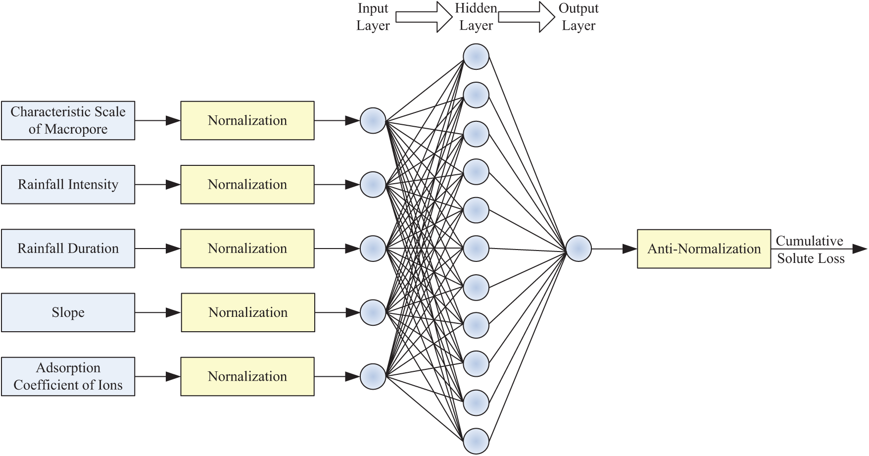
Figure 1: The structure of the improved BP neural network prediction method for slope solute loss considering soil macropores
After obtaining input and output variables, standardization pretreatment is conducted. The data of input and output is normalized into the range [0, 1]. The relatively large data still fall the place of large gradient of transfer function, so that the performance of the network training is improved. Here, the normalization method using the following equation.
where,
The middle layer of the neural network is hidden layer. The tangent transfer function tansig ( ) is used as its transfer function. If the number of neurons in the network hidden layer is too little, it will cause the discomfort of the network. On the other hand, if the number of neurons in the network hidden layer is too large, it can cause the adaptability of the network. In this paper, the number of the network hidden layer nodes is five. The variable of the network output layer is cumulative solute loss. The linear transfer function purelin( ) is used as its transfer function. The network output data is anti-normalized, so that the cumulative solute loss on slope is obtained.
In order to test the verify of the proposed model, an indoor slope water flow experiment was carried out in experimental tanks. The soil samples (referred to as Yangling soils) were, extracted from an experimental field site at Yangling District, Xi’an, China.
3.1 Soil Physical Characteristics
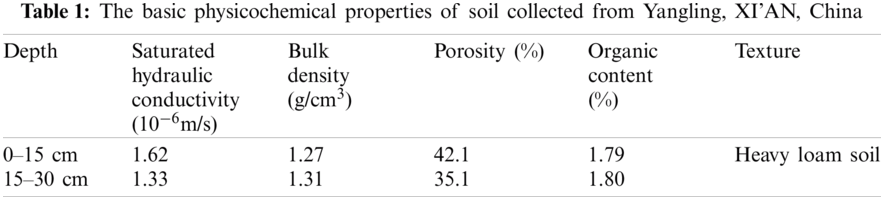
In order to accurately simulate actual field conditions, a stratified earth method is adopted, i.e., 0~15 cm is the first layer and 15~30 cm is the second layer. According to the U.S.D.A., the soil is classified as a heavy loam. The soil water characteristic curve, as shown in Fig. 2, was determined by a negative pressure meter method. Tab. 1 summaries the soil’s basic physicochemical properties.
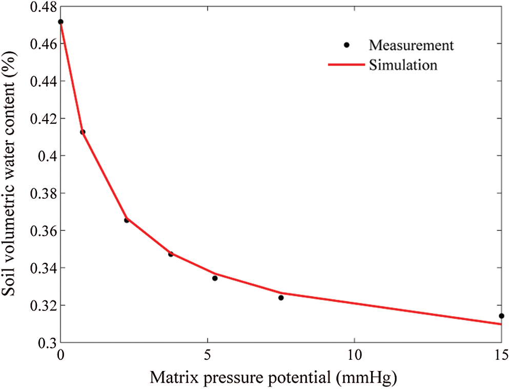
Figure 2: Soil water characteristic curve
Due to the complexity and diversity of the affecting factors, the soil water characteristic curve has not been established theoretically, and the relationship between the soil’s moisture and matric potential, along with the empirical formulas, are usually used to describe it. The common empirical formulas include Van-Genuchten, Brook-Corey, Kosugi and so on. In comparison with the other formula, the formula of Van-Genuchten can not only achieve a smooth curve, but also is universally applicable for most soil. Therefore, it is used to describe the hydraulics characteristics. The fitting curve can be established by means of the nonlinear function Isqcurvefit in Matlab and the average hydraulics characteristics value of the 11 kinds of different soil proposed by Rawls et al. [48], is regarded as the initial value of the input:
where,
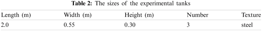
The experiment is conducted in three tanks with variable slope. The sizes of experimental tanks are shown in Tab. 2. A stratified filling method is adopted in order to accurately simulate actual field conditions.
The difference among the three experimental tanks lies in the underlying surfaces. Alfalfa is evenly grown in experimental tank 1. Alfalfa is a legume medicago, and also a perennial herb. Its root is rich, and it is an ideal plant to generate macropores. There are artificial macropores of 8 mm diameter in experimental tank 2. The plane distribution of the soil macropores is shown in Fig. 3. Where, “5”, “20” and “30”, represent that the depth of the macropores is 5, 20 and 30 cm, respectively. The production method of the artificial macropores is as follows. In the process of filling, according to the plane distribution of the soil macropores, a stainless steel pole is buried at different depths. After the filling is completed, the pole is pulled out gently. Experimental tank 3 is a bare slope. The underlying surfaces of three experimental tanks are shown in Fig. 4.
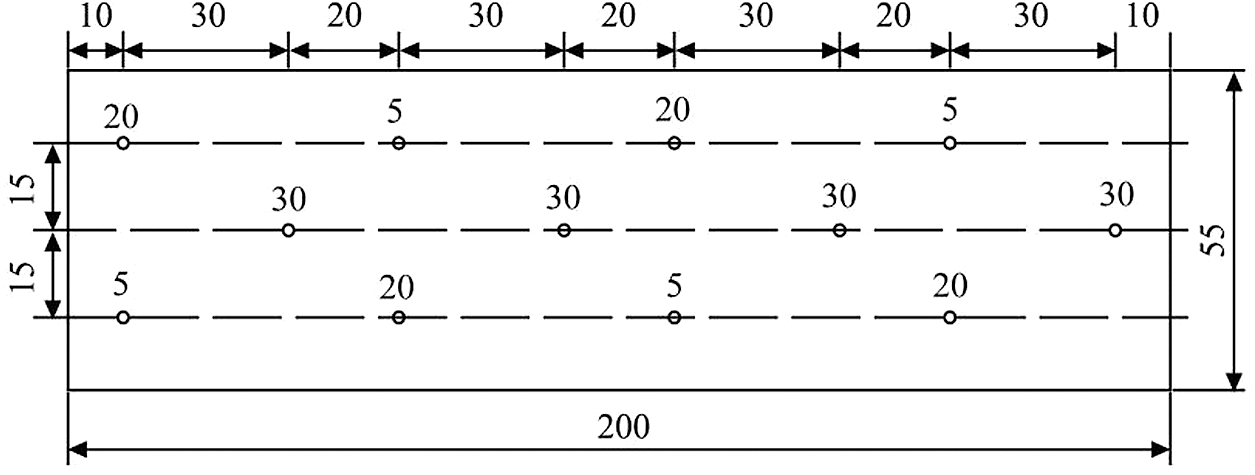
Figure 3: Plane distribution of the soil macropores
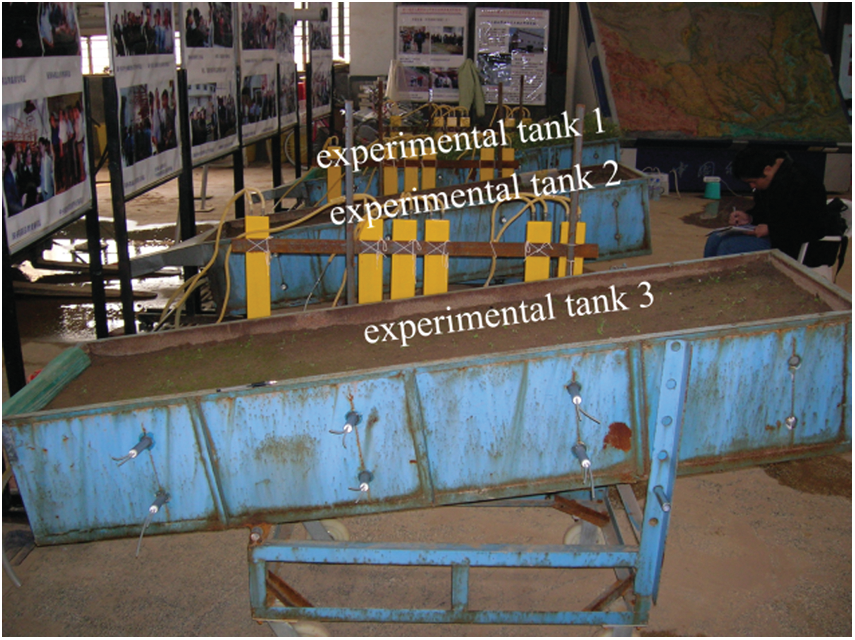
Figure 4: The underlying surface of the three experimental tanks
It takes a period of time for the plant to grow, therefore, before the rainfall, the same mass of water is added to tanks 1, 2 and 3. In the absence of rain, the experimental tanks are moved outdoors and are dried in the sun. In rainy weather, the experimental tanks are moved into the lab. The experiments can be conducted when the plants are mature.
In the process of the infiltration simulation, it is assumed that the distribution of the roots of Alfalfa is uniform. That is to say, the distribution of the soil macropores in experimental tank 1 is uniform. Only the artificial macropores are considered in tank 2. The soil in tank 3 is regarded as homogeneous soil without considering the soil macropores. In order to run the improved VIMAC model, the measured data of experimental tank 3 is applied to determine the infiltration parameters in the matrix flow domain; the measured data of experimental tank 1 is used to calculate the infiltration parameters in macropores flow domain and horizontal infiltration, and then the measured data of experimental tank 2 is used to test the infiltration model.
The outlets position of the surface runoff, the interflow and the groundwater runoff located above the bottom of the experimental tank are 0.35, 0.175 and 0 cm, respectively.
The optimal fittings for the measured surface runoff process, the measured undersurface runoff process and the profile of soil moisture are usually regarded as the criterion to judge the infiltration model. Here, the least square method between the measured undersurface runoff and the simulated undersurface runoff, is used as the standard.
3.3 The Artificial Rainfall Simulation System
The automatic rainfall simulation system, in the lateral jet zone of the State Key Laboratory of Soil Erosion and Dryland Farming on the Loess Plateau, is used as the artificial rainfall system. The actual rainfall height of the artificial simulation system is 16 m and the rainfall terminal speeds meet the natural rainfall characteristics’ requirement. The rainfall intensity control range is from 15 to 260 mm/h and the rainfall uniformity is above 85%.
A total of nine artificial rainfalls simulation are conducted for the three experimental tanks. Before each rainfall, 1.7g KBr is dissolved in the water, and 1000 mL solution is compounded and is uniformly spilled into the three experimental tanks. The surface runoff, interflow and groundwater runoff are measured using the gravimetric method. The soil volumetric water content is measured by the negative pressure meter method. Br− is conservative ion. There is not any movement of adsorption and transformation, only the movement of migration in the soil tank. The Br− concentration of water samples is measured by colorimetry. The Br− loss is calculated by the measured surface runoff multiplied by the Br− concentration of water samples at the same time.
In the process of the experiment, the raindrops make the surface soil in the experimental tank erode causing the geometry of soil macropores to be affected. Therefore, before every rainfall, according to the plane distribution of the macropores, stainless steel poles of different lengths are inserted into soil at different depths. Then, the poles are pulled out slowly, so that the characteristics of the macropores remain basically unchanged throughout the course of the experiment.
The impact of the soil macropores on slope solute loss is discussed before simulation model output results, in order to stress importance of the soil macropores.
4.1 The Impact of the Soil Macropores on Slope Solute Loss
During the nine rainfall events, the Br− loss carried by surface runoff is calculated. The results show that the Br− loss carried by the surface runoff on the slope with soil macropores is smaller than that on slope without soil macropores. For example, for a particular artificial rainfall event, the Br− loss carried by the surface runoff in experimental tanks 1, 2 and 3 is 42.54, 32.32 and 72.15 mg, respectively. For another particular artificial rainfall event, the Br− loss carried by the surface runoff in experiment tanks 1, 2 and 3 is 35.67, 30.62 and 38.37 mg, respectively. The reason may be that there were fast channels in the macropores slope, causing an increment of amount and speed of the leaching of the Br− and it being, carried by the water towards deeper layers, and thereby there was relatively small amounts of Br− on the surface. So that Br− loss carried by surface runoff on slope with soil macropores was relatively smaller. The dynamic change of the Br− loss rate in the surface runoff is shown in Fig. 5.
The Br− has a negative charge, which carries the same charge as the soil particles. The soil particles exclude from the Br−, so that the Br− easily separates from the soil particles and migrates with the solution. After the start of rainfall, due to raindrop’s striking the soil, the Br− on the soil surface mixes with the rainfall. One part of mixture migrates to the lower layer with water infiltration and, another part of mixture remains in the topsoil. After the start of the runoff, the topsoil Br− migrates with the runoff water. Due to the Br− having characteristics of easy migration, the Br− in the surface runoff decreases rapidly. The action of the raindrops hitting the soil and the runoff erosion causes, the upper layer of soil produces loss, and the lower layer of soil gradually supply to the Br− in surface runoff. Therefore, the Br− supplied to surface runoff decreases, so that the rate of the Br− loss in surface runoff decreases and enters into a stage of gentle change. Under the condition of raindrops striking the soil and the runoff erosion effect, the Br− observed in the upper layer of the soil will tend to be zero and the subsoil may begin to gradually supper Br−. So the rate that the Br− loss in surface runoff will diminish and go flat changes in different stages. In the early stage of rainfall, there is an obvious difference in the Br− loss amount. In the late stage of rainfall, the loss rate of the Br− tends to the same. In the prophase of rainfall, the Br− loss rate rapidly declines. With the increase of rainfall duration, the Br− loss rate tends to be low.
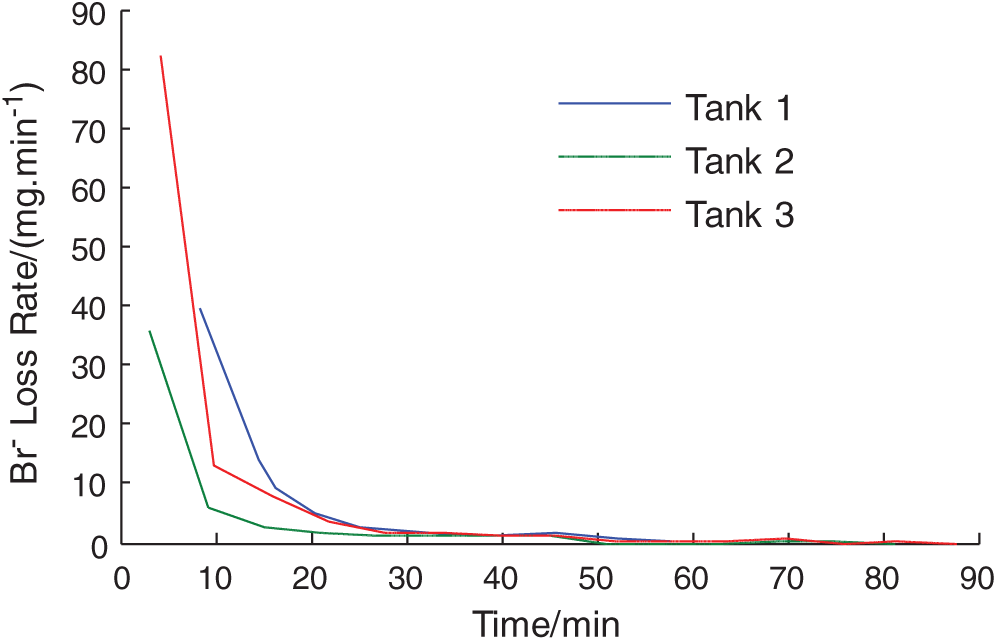
Figure 5: The dynamic change of the Br− loss rate in the surface runoff
4.2 The Model Validation Results
To verify the effectiveness of the proposed BP neural network model for slope solute loss considering soil macropores, the data of the solute cumulative loss with nine rainfalls and twenty seven slopes are measured. The input data of BP neural network method for slope cumulative solute loss is shown in Fig. 6. One hundred forty four sets of experiment data are obtained. It is used as the input data of the improved BP neural network prediction method for slope solute loss. The experimental data is divided into three parts, which is used to train the model, validate the model and test the model. A quarter of the experiment data is used to validate the model, and a quarter of the experiment data is used to test the model, and other experiment data is used to train the model. The training sample data, the validation sample data and the testing sample data are selected from the acquired experiment data using intervals method. The improved BP neural network prediction method for slope solute loss is trained using the sample data. The normalized experiment data is used for the training of the network.
The comparison of the mean squared error between gradient descent method and the proposed method is shown in Figs. 7 and 8. For both of the method, the number of network layer are three, the number of hidden layer nodes is five. As can be seen from Figs. 7 and 8, the convergence rate of solute loss prediction neural network using the proposed method is much faster than that of solute loss prediction neural network using gradient descent method. And the prediction accuracy of the proposed method is higher than that of gradient descent method. With the increase in the training time, the network error decreases. And the characteristics of validation error are similar to that of testing error. The results show that the proposed method is effective.
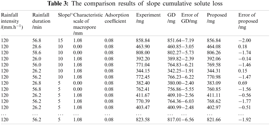
To further verify the effectiveness of the proposed method, the comparison of solute loss prediction performance between gradient descent method and the proposed method is analyzed. The comparison of solute loss prediction results is shown in Fig. 9. The comparison of slope solute loss prediction error is shown in Fig. 10. The prediction results of slope cumulative solute loss using the proposed method are shown in Tab. 3.
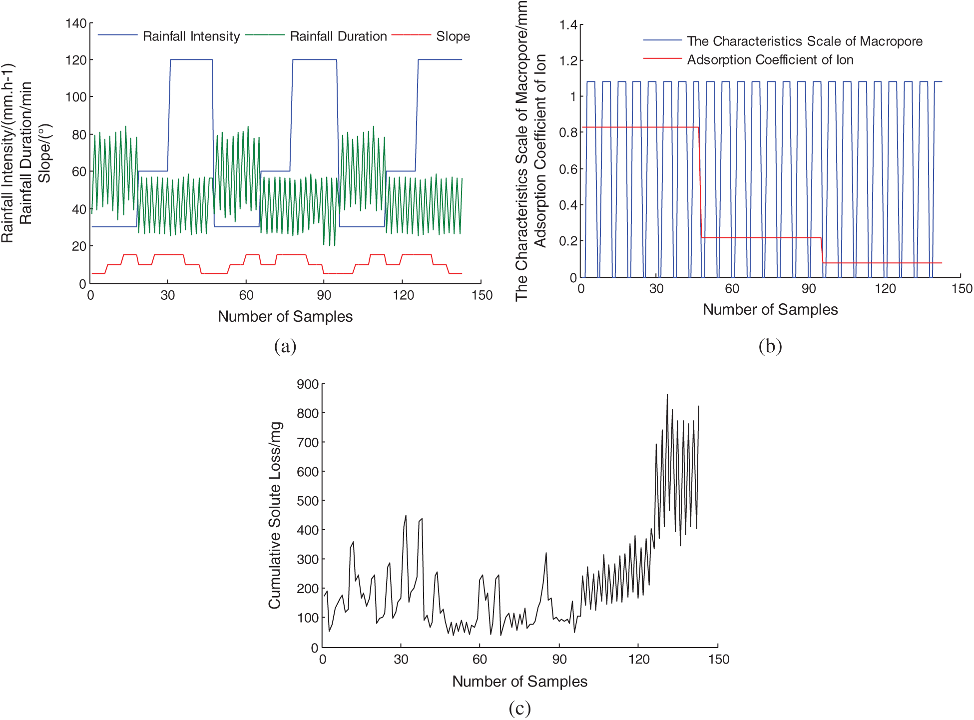
Figure 6: Input data of BP neural network model for slope solute loss considering soil macropores (a) Rainfall intensity, rainfall duration and slope (b) The characteristics scale of macropore and adsorption coefficient (c) The cumulative solute loss
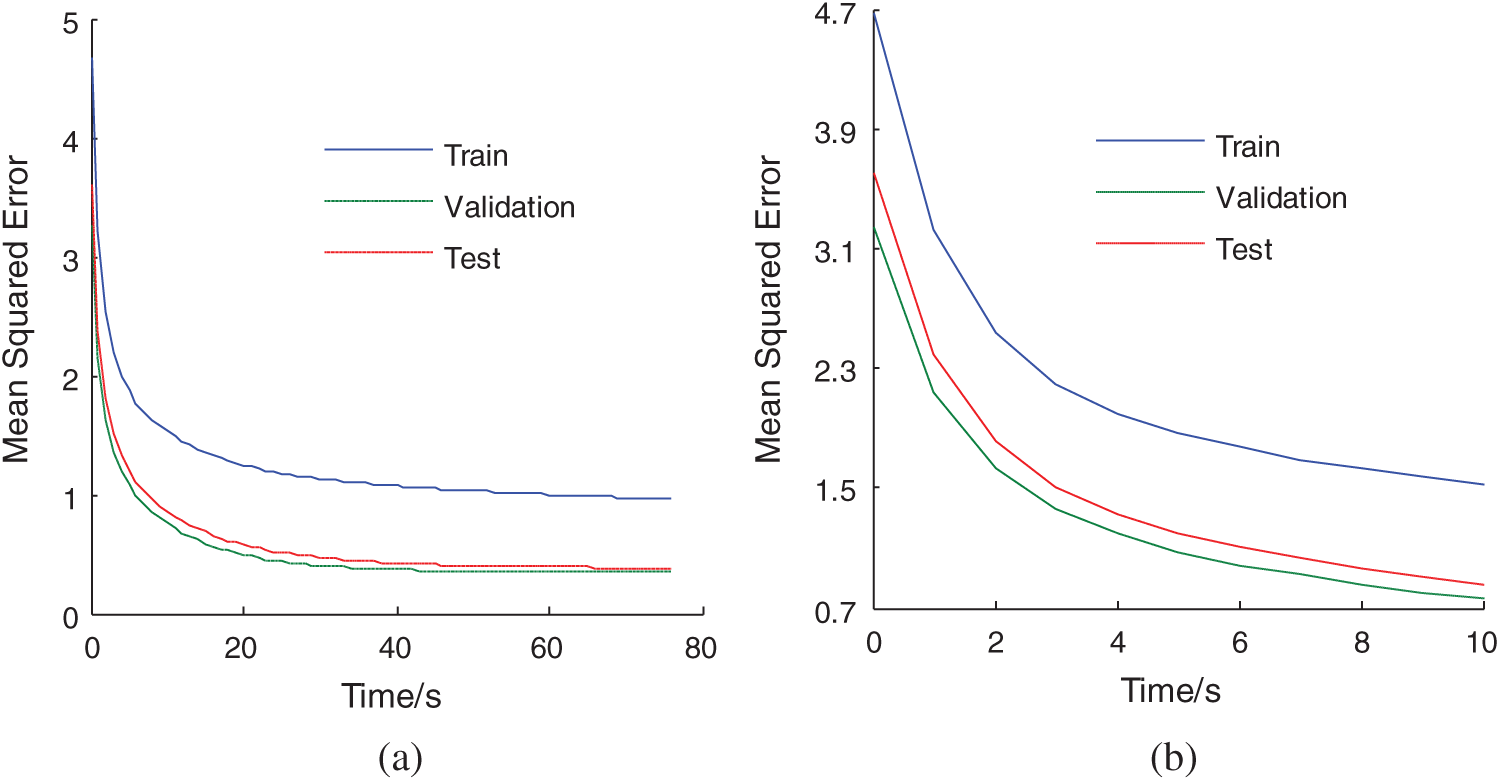
Figure 7: The mean squared error of gradient descent method (a) The whole comparison curve (b) The partial comparison curve
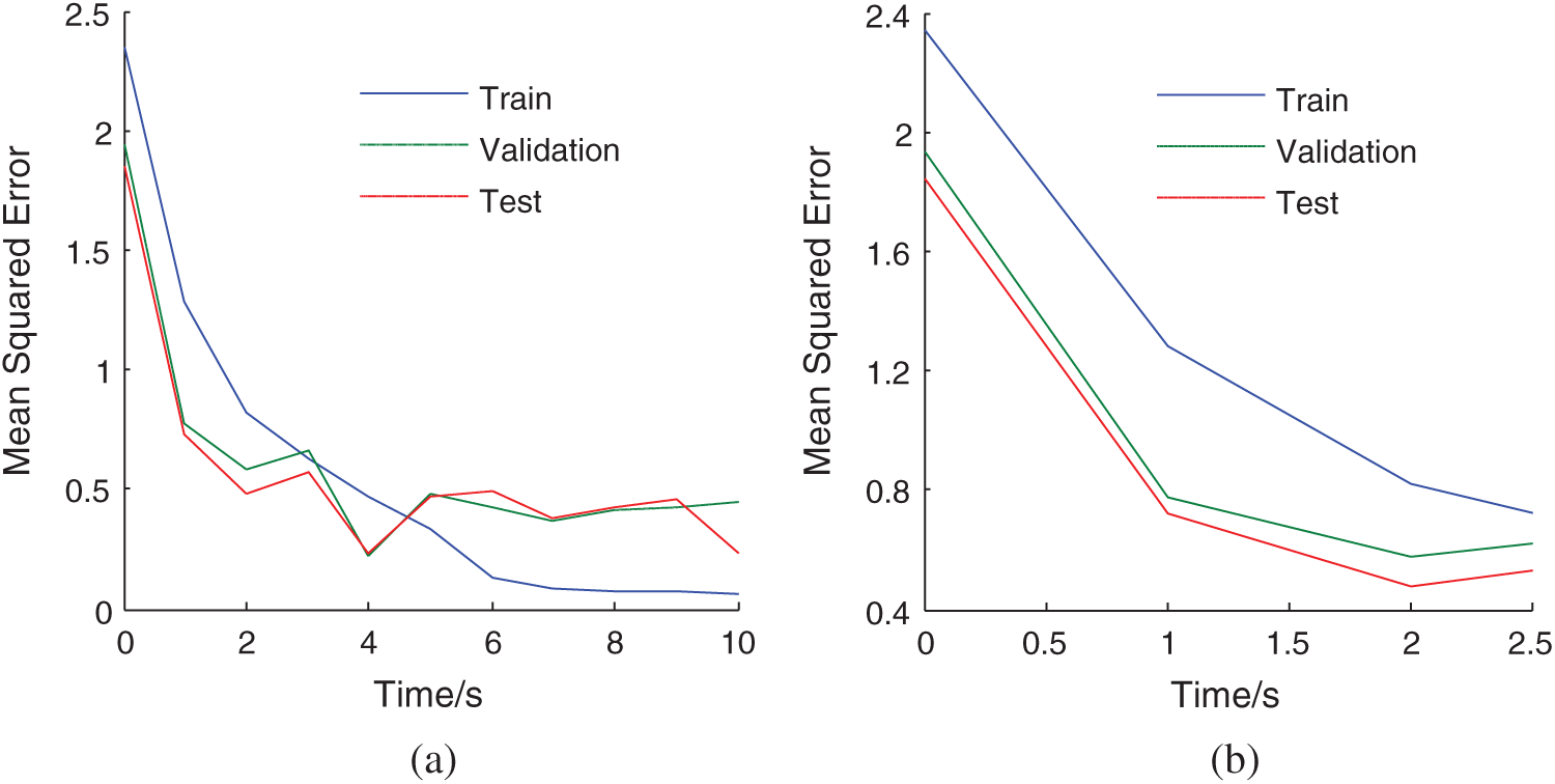
Figure 8: The mean squared error of the proposed method (a) The whole comparison curve (b) The partial comparison curve
In Tab. 3, “Experiment” represents measured cumulative solute loss, “GD” represents the cumulative solute loss results using gradient descent method, “Error of GD” represents the absolute error of the cumulative solute loss results using gradient descent method, “Proposed” represents the cumulative solute loss results using the proposed method, “Error of proposed” represents the absolute error of the cumulative solute loss results using the proposed method.
As can be seen from Figs. 9, 10 and Tab. 3, slope solute loss prediction error using gradient descent BP neural network method is very large, and slope solute loss prediction error using the proposed method is little. The maximum absolute error of slope cumulative solute loss using gradient descent method is 7.19 mg, and that of the proposed method is within a range of 2 mg. The results show that the effectiveness of the proposed method again.
This study of slope solute loss model considering soil macropores, is significant to the agricultural management of non-point source pollution and nutrient loss. In this study, a new improved BP neural network prediction method for slope solute loss considering soil macropores based on Levenberg–Marquardt training algorithm is proposed in this paper. The input variables include: rainfall intensitys rainfall durations slopes the characteristic scale of the soil macropores, and the adsorption coefficient of ion. The output variable is the cumulative solute loss on the slope. The rainfall intensity and duration are directly obtained from the automatic rainfall simulation system. The slope is obtained by measuring the elevation of the experimental tank, as well as the length of the experimental tank. The adsorption coefficient of ion is obtained by adsorption experiments and the relevant references. The characteristic scale of the soil macropores is obtained by the calculation of the improved VIMAC model simulation. In order test the feasibility of this model, artificial rainfall simulation experiments are conducted in indoor experimental tanks. In addition, the impact of the soil macropores on slope solute loss has been further confirmed before the simulation.

Figure 9: The comparison of slope cumulative solute loss (a) The whole comparison curve (b) Partial comparison curve one (c) Partial comparison curve two
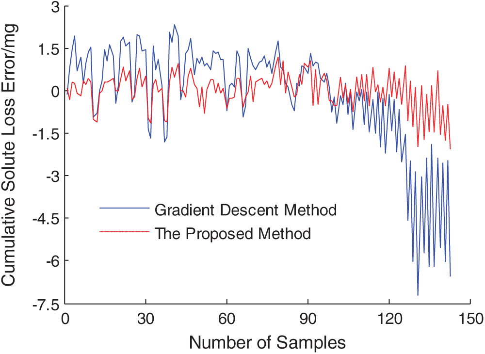
Figure 10: Error comparison of slope cumulative solute loss
Our results demonstrate, that the total loss and the average loss rate of the Br− carried by the surface runoff with soil macropores are less than those without soil macropores. In the early stage of the rainfall, there is an obvious difference in the Br− loss total amount. In the late stage of the rainfall, the loss rate of the Br− tends to the same. The error analysis and the performance comparison between the proposed method and traditional gradient descent method are done. The results show that the convergence rate of neural network for slope cumulative solute loss prediction using the proposed method is much faster than that of neural network for slope cumulative solute loss prediction using gradient descent method. And the prediction accuracy of the proposed method is higher than that of gradient descent method. The proposed method meets the requirements of application. However, if different sizes experimental tanks are used, the result may vary, which requires further research.
Funding Statement: This research was financially supported by the National Natural Science Foundation of China (No. 41301037), the Natural Science Foundation of the Jiangsu Higher Education Institutions of China (No. 11KJB170008) and Innovation and Entrepreneurship Training Program for College Students in Jiangsu Province (No. 201910300106Y). For the help in carrying out the experiments, I wish to thank for Professor Rui Xiaofang, Hohai University, China.
Conflicts of Interest: The authors have declared that they have no conflicts of interest to report regarding the present study.
1. K. Beven and P. Germann, “Macropores and water flow in soils,” Water Resource Research, vol. 18, no. 5, pp. 1311–1325, 1982. [Google Scholar]
2. Y. Zhang, W. Zhao, J. He and L. Fu, “Soil susceptibility to macropore flow across a desert-oasis ecotone of the Hexi Corridor, Northwest China,” Water Resources Research, vol. 54, no. 2, pp. 1281–1294, 2018. [Google Scholar]
3. X. Rui, Runoff generation mechanism and watershed runoff generation. in Principle of Hydrology, 1st ed., vol. 8. Beijing, China: Higher Education Press, pp. 155, 2013. [Google Scholar]
4. J. X. Tong and J. Z. Yang, “Analysis of soluble chemical transfer by runoff water in filed,” Journal of Hydrodynamics, vol. 20, no. 3, pp. 382–390, 2008. [Google Scholar]
5. X. C. Zhang, D. Norton, T. Lei and M. A. Nearing, “Coupling mixing zone concept with convection-diffusion equation to predict chemical transfer to surface runoff,” Transactions of ASAE, vol. 42, no. 4, pp. 987–994, 1999. [Google Scholar]
6. R. Wallach, G. Galina and J. Rivlin, “A comprehensive mathematical model for transport of soil-dissolved chemicals by overland flow,” Journal of Hydrology, vol. 247, no. 1–2, pp. 85–99, 2001. [Google Scholar]
7. M. T. Walter, B. Gao and J. Y. Parlange, “Modeling soil solute release into runoff with infiltration,” Journal of Hydrology, vol. 347, no. 3–4, pp. 430–437, 2007. [Google Scholar]
8. Q. Wang and H. Wang, “Analysis on the feature of effective mixing depth model for soil solute transporting with surface runoff on loess slope,” Hydrological Processes, vol. 41, no. 6, pp. 671–676, 2010. [Google Scholar]
9. W. Dong, Q. Wang, B. Zhou and Y. Shan, “A simple model for the transport of soil-dissolved chemicals in runoff by raindrops,” Catena, vol. 101, no. 1, pp. 129–135, 2013. [Google Scholar]
10. N. W. Haws, P. S. C. Rao, J. Simunek and I. C. Poyer, “Single-porosity and dual porosity modeling of water flow and solute transport in subsurface-drained fields using effective field-scale parameters,” Journal of Hydrology, vol. 313, no. 3–4, pp. 257–273, 2005. [Google Scholar]
11. A. Elci and F. Molz, “Identification of lateral macropore flow in a forested riparian wetland through numerical simulation of a subsurface tracer experiment,” Water Air Soil Pollution, vol. 197, no. 1–4, pp. 149–164, 2009. [Google Scholar]
12. E. Lamy, L. Lassabatere, B. Bechet and H. Andrieu, “Modeling the influence of an artificial macropore in sandy columns on flow and solute transfer,” Journal of Hydrology, vol. 376, no. 3–4, pp. 392–402, 2009. [Google Scholar]
13. P. Jørgensen, K. Mosthaf and M. Rolle, “A large undisturbed column method to study flow and transport in macropores and fractured media,” Groundwater, vol. 57, no. 6, pp. 951–961, 2019. [Google Scholar]
14. F. Abbasi, J. Feyen and M. T. Van Genuchten, “Two-dimensional simulation of water flow and solute transport below furrows: Model calibration and validation,” Journal of Hydrology, vol. 290, no. 1–2, pp. 63–79, 2004. [Google Scholar]
15. L. Luo, H. Lin and S. Li, “Quantification of 3-D soil macropore networks in different soil types and land uses using computed tomography,” Journal of Hydrology, vol. 393, no. 1–2, pp. 53–64, 2010. [Google Scholar]
16. F. S. J. Martínez, M. A. Martín, F. J. Caniego, M. Tuller and A. Guber, “Multifractal analysis of discretized X-ray CT images for the characterization of soil macropore structures,” Geoderma, vol. 156, no. 1–2, pp. 32–42, 2010. [Google Scholar]
17. A. Tiktak, R. F. A. Hendriks, J. J. T. I. Boesten and A. M. A. Linden, “A spatially distributed model of pesticide movement in Dutch macroporous soils,” Journal of Hydrology, vol. 471, no. 11, pp. 316–327, 2012. [Google Scholar]
18. S. Feng, H. Liu, K. Wang, R. Zhang and Z. Tang, “Investigation into preferential flow in natural unsaturated soils with field multiple-tracer infiltration experiments and the active region model,” Journal of Hydrology, vol. 508, no. 16, pp. 137–146, 2014. [Google Scholar]
19. S. G. Diego, P. R. Paula and V. J. Laura, “A new method to trace colloid transport pathways in macroporous soils using X-ray computed tomography and fluorescence macrophotography,” European Journal of Soil Science, vol. 70, no. 3, pp. 431–442, 2019. [Google Scholar]
20. R. S. Walton, R. E. Volker, K. L. Bristow and K. R. J. Smettem, “Experimental examination of solute transport by surface runoff from low-angle slopes,” Journal of Hydrology, vol. 233, no. 1–4, pp. 19–36, 2000. [Google Scholar]
21. B. Gao, M. T. Walter, T. S. Steenhuis, J. Y. Parlange, B. K. Richards et al., “Investigating raindrop effects on transport of sediment and nonsorbed chemicals from soil to surface runoff,” Journal of Hydrology, vol. 308, no. 1–4, pp. 313–320, 2005. [Google Scholar]
22. C. R. Yu, B. Gao, R. Muñoz-Carpena, Y. Tian, L. Wu et al., “A laboratory study of colloid and solute transport in surface runoff on saturated soil,” Journal of Hydrology, vol. 402, no. 1–2, pp. 159–164, 2011. [Google Scholar]
23. A. Kavian, A. Alipour, K. Soleimani, L. Gholami, P. Smith et al., “The increase of rainfall erosivity and initial soil erosion processes due to rainfall acidification,” Hydrological Processes, vol. 33, no. 2, pp. 261–270, 2019. [Google Scholar]
24. L. Lu, J. Wu and J. Wang, “Monte carlo modeling of solute transport in a porous medium with multi-scale heterogeneity,” Advances in Water Science, vol. 19, no. 3, pp. 333–338, 2008. [Google Scholar]
25. A. B. Çolak, “A novel comparative analysis between the experimental and numeric methods on viscosity of zirconium oxide nanofluid: Developing optimal artificial neural network and new mathematical model,” Powder Technology, vol. 381, no. May, pp. 338–351, 2021. [Google Scholar]
26. N. Effendy, S. H. A. Aziz, H. M. Kamari, M. H. M. Zaid and S. A. A. Wahab, “Artificial neural network prediction on ultrasonic performance of bismuth-tellurite glass compositions,” Journal of Materials Research and Technology, vol. 9, no. 6, pp. 14082–14092, 2020. [Google Scholar]
27. W. Sun, G. Zhang, X. Zhang, X. Zhang and N. Ge, “Fine-grained vehicle type classification using lightweight convolutional neural network with feature optimization and joint learning strategy,” Multimedia Tools and Applications, pp. 1–14, 2020. https://doi.org/10.1007/s11042-020-09171-3. [Google Scholar]
28. X. Zhang, X. Chen, W. Sun and X. He, “Vehicle re-identification model based on optimized denseNet121 with joint loss,” Computers, Materials & Continua, vol. 67, no. 3, pp. 3933–3948, 2021. [Google Scholar]
29. X. Zhang, H. Wu, W. Sun and S. K. Jha, “A fast and accurate vascular tissue simulation model based on point primitive method,” Intelligent Automation & Soft Computing, vol. 27, no. 3, pp. 873–889, 2021. [Google Scholar]
30. X. Zhang, W. Zhang, W. Sun, T. Xu and S. K. Jha, “A robust watermarking scheme based on ROI and IWT for remote consultation of COVID-19,” Computers, Materials & Continua, vol. 64, no. 3, pp. 1435–1452, 2020. [Google Scholar]
31. X. Zhang, X. Yu, W. Sun and A. Song, “Soft tissue deformation model based on marquardt algorithm and enrichment function,” Computer Modeling in Engineering & Sciences, vol. 124, no. 3, pp. 1131–1147, 2020. [Google Scholar]
32. X. Zhang, X. Yu, W. Sun and A. Song, “An optimized model for the local compression deformation of soft tissue,” KSII Transactions on Internet and Information Systems, vol. 14, no. 2, pp. 671–686, 2020. [Google Scholar]
33. X. Zhang, H. Wu, W. Sun and C. Yuan, “An optimized mass-spring model with shape restoration ability based on volume conservation,” KSII Transactions on Internet and Information Systems, vol. 124, no. 3, pp. 1738–1756, 2020. [Google Scholar]
34. H. Wang, “Mechanism and simulation of nutrient transport on loess slope land during rainfall,” Ph.D. dissertation. Northwest A&F University, Yang Ling, Shanxi, China, 2006. [Google Scholar]
35. X. Zhang, J. Feng and T. Yang, “Lattice Boltzmann method for overland flow studies and its experimental validation,” Journal of Hydraulic Research, vol. 53, no. 5, pp. 561–575, 2015. [Google Scholar]
36. T. Fu, J. Ni, C. Wei and D. Xie, “Research on nutrient loss from terra gialla soil in three gorges region under different rainfall intensity,” Journal of Soil and Water Conservation, vol. 16, no. 2, pp. 33–35, 2002. [Google Scholar]
37. B. Gao, M. T. Walter, T. S. Steenhuis, W. L. Hogarth and J. Y. Parlange, “Rain induced chemical transport from soil to runoff: Theory and experiments,” Journal of Hydrology, vol. 295, no. 1–4, pp. 291–304, 2004. [Google Scholar]
38. T. Guo, Q. Wang, D. Li, J. Zhuang and L. Wu, “Flow hydraulic characteristic effect on sediment and solute transport on slope erosion,” Catena, vol. 107, no. 8, pp. 145–153, 2013. [Google Scholar]
39. X. Chen, X. Fan and D. Li, “Phosphorus form in surface runoff and its affecting factors in hilly upland,” China Environmental Science, vol. 20, no. 3, pp. 284–288, 2000. [Google Scholar]
40. X. C. Zhang, L. D. Norton and M. Hickman, “Rain pattern and soil moisture content effects on Atrazine and Metolachlor losses in runoff,” Journal of Environmental Quality, vol. 26, no. 6, pp. 1539–1547, 1997. [Google Scholar]
41. A. Ghafoor, J. Koestel, M. Larsbo, J. Moeys and N. Jarvis, “Soil properties and susceptibility to preferential solute transport in tilled topsoil at the catchment scale,” Journal of Hydrology, vol. 492, pp. 190–199, 2013. [Google Scholar]
42. S. E. Allaire-Leung, S. C. Gupta and J. F. Moncrief, “Water and solute movement in soil as influenced by macropore characteristics: 1,” Macropore Continuity, Journal of Contaminant Hydrology, vol. 41, no. 3–4, pp. 283–301, 2000. [Google Scholar]
43. X. Zhang, J. Feng, F. Liu and C. Zhang, “Analysis of effect of soil macropore on slope runoff yield and concentration and solute transport,” Water Resources and Power, vol. 27, no. 1, pp. 32–36, 2009. [Google Scholar]
44. X. Zhang, J. Feng, Y. Gao and N. Liu, “Influences of slope on runoff and concentration and solute transport under different rainfall intensities,” Bulletin of Soil and Water Conservation, vol. 30, no. 2, pp. 119–123, 2010. [Google Scholar]
45. S. Hu and C. Jin, “Theoretical analysis and experimental study on the critical slope of erosion,” Acta Geographical Sinica, vol. 54, no. 4, pp. 347–356, 1999. [Google Scholar]
46. X. Zhang, “Study on runoff yield and concentration model and solute loss model in macroporous soils and experiment verification,” Ph.D. dissertation. Hohai university, Nanjing, Jiangsu, China, 2010. [Google Scholar]
47. G. Roberto, “Preferential flow in macroporous swelling soil with internal catchment: Model development and applications,” Journal of Hydrology, vol. 269, no. 3–4, pp. 150–168, 2002. [Google Scholar]
48. W. J. Rawls, D. L. Brakensiek and K. E. Saxton, “Estimating of soil water properties,” Transaction ASAE, vol. 25, no. 5, pp. 1316–1320, 1982. [Google Scholar]
 | This work is licensed under a Creative Commons Attribution 4.0 International License, which permits unrestricted use, distribution, and reproduction in any medium, provided the original work is properly cited. |