Computers, Materials & Continua DOI:10.32604/cmc.2021.017836
Article

Implementation of Legendre Neural Network to Solve Time-Varying Singular Bilinear Systems

V. Murugesh1, B. Saravana Balaji2,*, Habib Sano Aliy3, J. Bhuvana4, P. Saranya5 andino Maseleno6, K. Shankar7, and A. Sasikala8

1Department of Computer Science, College of Informatics, Bule Hora University, PO Box 144, Ethiopia
2Department of Information Technology, Lebanese French University, Erbil, 44001, Iraq
3Deptartment of Logistics and Supply Chain Management, Arba Minch University, Sawla Campus, PO Box 13, Ethiopia
4Department of MCA, School of Computer Science and IT, Jain (Deemed to be) University, Bangalore, 560069, India
5Department of Computer Science and Engineering, SRM Institute of Science and Technology, Chennai, 603203, India
6Department of Information Systems, STMIK Pringsewu, Lampung, Indonesia
7Department of Computer Applications, Alagappa University, Karaikudi, 630003, India
8Department of EEE, Sri Sairam Institute of Technology, Chennai, 600044, India
*Corresponding Author: B. Saravana Balaji. Email: saravanabalaji.b@lfu.edu.krd
Received: 13 February 2021; Accepted: 03 May 2021

Abstract: Bilinear singular systems can be used in the investigation of different types of engineering systems. In the past decade, considerable attention has been paid to analyzing and synthesizing singular bilinear systems. Their importance lies in their real world application such as economic, ecological, and socioeconomic processes. They are also applied in several biological processes, such as population dynamics of biological species, water balance, temperature regulation in the human body, carbon dioxide control in lungs, blood pressure, immune system, cardiac regulation, etc. Bilinear singular systems naturally represent different physical processes such as the fundamental law of mass action, the DC motor, the induction motor drives, the mechanical brake systems, aerial combat between two aircraft, the missile intercept problem, modeling and control of small furnaces and hydraulic rotary multi-motor systems. The current research work discusses the Legendre Neural Network’s implementation to evaluate time-varying singular bilinear systems for finding the exact solution. The results were obtained from two methods namely the RK-Butcher algorithm and the Runge Kutta Arithmetic Mean (RKAM) method. Compared with the results attained from Legendre Neural Network Method for time-varying singular bilinear systems, the output proved to be accurate. As such, this research article established that the proposed Legendre Neural Network could be easily implemented in MATLAB. One can obtain the solution for any length of time from this method in time-varying singular bilinear systems.

Keywords: Time-varying singular bilinear systems; RK-butcher algorithm; legendre neural network method

1  Introduction

Differential Equations (DEs) are algebraic relations that exist between functions and their derivatives. These DEs are the backbone of any sort of physical system. Partial differential equations (PDE) or ordinary differential equations (ODE) are the basis upon which most of the chemistry, physics, math, engineering etc., are modeled. In most cases, it is not simple to get an analytical solution for DEs. Therefore, researchers started considering new and dynamic numerical methods to approximate their solutions.

Numerical methods have few limitations, for instance, high computational cost. However, they are widely used for resolving DEs, and they evolved since the first differential equation was derived. Finite differences, finite elements, finite volumes and spectral methods are some of the conventional methods available for spatial discretization of Partial Differential Equations (PDEs) [1]. In this case of discretizing Ordinary Differential Equations (ODEs), some of the following conventional methods are applied i.e., the Euler Method, the Runge–Kutta Method, the RK-Gill Method [2] and the RK-Butcher Algorithm [3].

Artificial Intelligence (AI) experienced rapid development in recent years due to the researchers shifted their attention towards neural network methods [4]. Artificial Neural Networks (ANN) are applied in a wide of domains such as control systems [5], image processing techniques [6] and pattern recognition [7] since they produce promising output. With a proven track record, neural network methods, especially neural network function approximation capabilities, are applied to solve DEs through neural network models.

Legendre Neural Network was leveraged in the study conducted by Mall et al. [8], in which a novel method was proposed as a solution for ODE. To solve two DEs such as Linear Coefficients Delay Differential-Algebraic Equations and Singularly Perturbed DE [9], Legendre Neural Network was proposed by Liu et al. [10]. Yang et al. [11] used Legendre Neural Network-based algorithm for elliptical partial DEs. In the research conducted by Chen et al. [12], the researchers used Block Trigonometric Exponential Neural Network to find a probable solution for Continuous-Time Model. A new algorithm was proposed by Toni Schneidereit et al. based on Artificial Neural Network to resolve ODs [13].

In the current research paper, the author proposes a novel approach to resolve time-varying singular bilinear systems with the help of the highly accurate Legendre Neural Network method [14].

2  Legendre Neural Networks

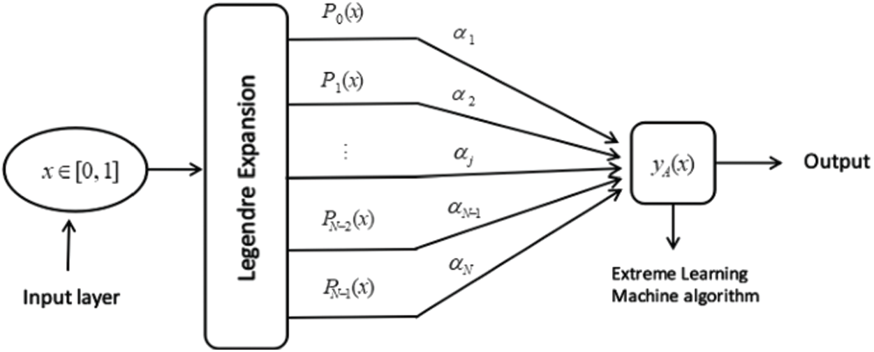
There are two components present in single layers Legendre Neural Network such as input node and output node [15]. Its functional expansion depends on Legendre polynomials. Legendre polynomials constitute a set of orthogonal polynomials which are obtained as a solution for Legendre differential equations. Legendre polynomials are simply denoted Ln(u) in which n is the order of polynomial whereas u lies between −1 and 1. Legendre polynomials are a group of orthogonal polynomials and attained to resolve Legendre differential equations. Fig. 1 shows the structure of the Legendre Neural Network.

Figure 1: Architecture of legendre neural network

Having its functional expansion based on Legendre polynomial Pn(x), Legendre Neural Network for a single layer has one input and one output. The mathematical model for Legendre Neural Network for N nodes of a polynomial Pn(x) is as follows

yA(x)=∑j=1Nαjpj−1(wjx+bj) (1)

Here, the network’s input value is denoted by x, the output is denoted by yA, the weight of the input node of jth hidden node is denoted via wj, bj corresponds to the threshold for jth hidden node, and finally, the weight vector of the jth hidden node is denoted by αj. To simplify the Eq. (1), let us take wj=1 and bj=0, then the model in the Eq. (1) becomes

yA(x)=∑j=1Nαjpj−1(x) (2)

As per the universal approximation theorem, Singularly Perturbed Differential Equations (SPDEs) represent its analytical solution, whereas yA(x) represents its approximate solution

‖y(x)−yA(x)‖=‖y(x)−∑j−1Nαjpj−1(x)‖≤∈ (3)

L∈yA(x)=Con∂I (4)

Here, the intervals are discretized, which denotes the boundary points. The weight αj can be solved as given herewith.

(α)=[f1f2f3⋮c] (5)

This can be described simply as follows

Hα=F (6)

H matrix is the first left term in Eq. (4) that corresponds to the neural network’s output matrix after the linear L∈ operator and B f is the first proper Eq. (4). To mitigate the error between proper solution y(x) and approximate solution yA(x), the optimization should be done by using extreme Machine Learning (ML) algorithm [16] as given as follows.

min‖H(α)−f‖ (7)

3  Time-Varying Singular Bilinear Systems

Here, the first-order time-varying singular system is considered.

Kx˙(t)=Ax(t)+B(t)u(t) (8)

In this equation x(0)=x0, K corresponds to n×n singular matrix, whereas n×n matrix is denoted by A and n×r matrix is denoted by B. The n-state vectors are denoted by x(t), while the r-input vector corresponds to u(t).

Based on the above discussion, the time-varying singular bilinear system is rewritten in the following form.

E(t)x˙(t)=A(t)x(t)+∑i=1qNi(t)x(t)ui(t)+B(t)u(t) (9)

The rewritten form of Eq. (9) is given below.

E(t)x˙(t)=(A(t)+∑i=1qNi(t)ui(t))x(t)+B(t)u(t) (10)

Here, E(t)∈Rn×n denotes the singular matrix whereas the state corresponds to x(t)∈Rn, control.

u(t)∈Rq, A(t)∈Rn×n, B(t)∈Rn×q. Ni(t)∈Rn×n and ui(t),i=1,2,3,…,q, are the components of u(t). From this equation, the response x(t) 0≤t≤ti, should be calculated.

It is challenging to solve a time-varying singular bilinear system compared to its counterpart i.e., time-invariant singular bilinear system [17]. So, various researchers attempted different transformation methods to get rid of this challenge. The current research study leveraged Legendre Neural Network to find a highly accurate solution for a time-varying singular bilinear system [18].

4  Simulation Example

In this research work, the author considered a time-varying singular bilinear system as proposed earlier [19,20].

E(t)=[0−t010t010],A(t)=[−2t10−42−2t01],N1(t)=[1−t103−22t0−2],B(t)=[213]T,u(t)=1,with initial condition x(0)=[1225]T} (11)

If Eq. (5) is solved, then the exact solution for x(t) is as shown below

x(t)=[(2−t)(exp⁡(−t2)+exp⁡(t))+82exp⁡(−t2)−exp⁡(t)+1exp⁡(−t2)+exp⁡(t)+3] (12)

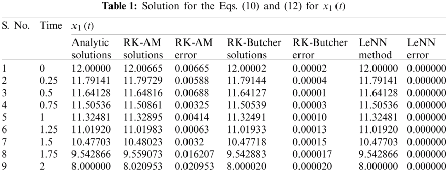
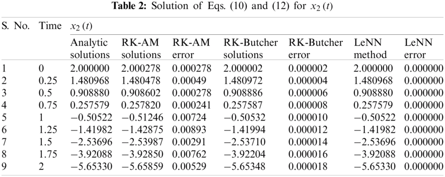
Legendre Neural Network was used to further assess the discrete solution for Eq. (10), and in this stage, 0.25 is considered the step size (t). The results attained from different methods such as the RK-Butcher algorithm and the Runge Kutta Arithmetic Mean Method (RKAM) were compared with that of the solution attained from Legendre Neural Network. Tabs. 1 and 2 show the results and the analytic solution determined using Eq. (12). These tables further shows the error between analytic solution and discrete solution.

5  Conclusions

Legendre Neural Network obtained highly accurate discrete solutions compared to other methods such as the RK-Butcher algorithm and the Runge Kutta Arithmetic Mean Method (RKAM). It can be observed from Tabs. 1–2 that Legendre Neural Network Method attained only minimal absolute error in contrast to RKAM and RK-Butcher Algorithms because these algorithms produced a considerable error. To conclude, the current study results established that Legendre Neural Network is a promising candidate to evaluate time-varying singular bilinear systems.

Funding Statement: The authors received no specific funding for this study.

Conflicts of Interest: The authors declare that they have no conflicts of interest to report regarding the present study.

References

 1.  T. Schneidereit and M. Breu, “Solving ordinary differential equations using artificial neural networks—A study on the solution variance,” in 21st Conf. on Scientific Computing, Slovakia, pp. 10–15, 2020. [Google Scholar]

 2.  V. Murugesh and K. Murugesan, “Comparison of numerical integration algorithms in raster CNN simulation,” in Lecture Notes in Computer Science, vol. 3285. Heidelberg: Springer-Verlag, pp. 115–122, 2004. [Google Scholar]

 3.  V. Murugesh, K. Murugesan and K. T. Kim, “Simulation of non-linear singular systems using RK-butcher algorithm,” in Communications in Computer and Information Science, vol. 206. Heidelberg: Springer-Verlag, pp. 625–632, 2011. [Google Scholar]

 4.  V. Murugesh and K. Murugesan, “Simulation of time-multiplexing CNN with numerical integration algorithms,” in Lecture Notes in Computer Science. vol. 3991. Heidelberg: Springer-Verlag, 2006. [Google Scholar]

 5.  V. Murugesh and K. Murugesan, “RK-Butcher algorithms for singular system based electronic circuit,” International Journal of Computer Mathematics, vol. 86, no. 3, pp. 523–536, 2009. [Google Scholar]

 6.  V. Murugesh, “Raster cellular neural network simulator for image processing applications with numerical integration algorithms,” International Journal of Computer Mathematics, vol. 86, no. 7, pp. 1215–1221, 2009. [Google Scholar]

 7.  V. Murugesh, “Image processing applications via time-multiplexing cellular neural network simulator with numerical integration algorithms,” International Journal of Computer Mathematics, vol. 87, no. 4, pp. 840–848, 2010. [Google Scholar]

 8.  S. Mall and S. Chakraverty, “Application of legendre neural network for solving ordinary differential equations,” Applied Soft Computing, vol. 43, no. 4, pp. 347–356, 2016. [Google Scholar]

 9.  H. Liu, J. Song, H. Liu, J. Xu and L. Li, “Legendre neural network for solving linear variable coefficients delay differential-algebraic equations with weak discontinuities,” Advances in Applied Mathematics and Mechanics, vol. 13, no. 1, pp. 101–118, 2021. [Google Scholar]

10. H. Liu, B. Xing, Z. Wang and L. Li, “Legendre neural network method for several classes of singularly perturbed differential equations based on mapping and piecewise optimization technology,” Neural Processing Letters, vol. 3, no. 3, pp. 2891–2913, 2020. [Google Scholar]

11. Y. Yang, M. Hou, H. Sun, T. Zhang, F. Weng et al., “Neural network algorithm based on legendre improved extreme learning machine for solving elliptic partial differential equations,” Soft Computing, vol. 2, pp. 24–38, 2020. [Google Scholar]

12. Y. Chen, C. Yi, X. Xie, M. Hou and Y. Cheng, “Solution of ruin probability for continuous time model based on block trigonometric exponential neural network,” Symmetry, vol. 12, no. 6, pp. 1–20, 2020. [Google Scholar]

13. G. B. Huang, O. Y. Zhu and C. K. Siew, “Extreme learning machine: Theory and applications,” Neurocomputing, vol. 70, no. 1, pp. 489–501, 2006. [Google Scholar]

14. B. Sepehrian and M. Razzaghi, “State analysis of time-varying singular bilinear systems by single-term walsh series,” International Journal of Computer Mathematics, vol. 80, no. 80, pp. 413–418, 2003. [Google Scholar]

15. V. Murugesh and K. T. Kim, “An efficient edge detection using raster CNN simulator,” in Lecture Notes in Computer Science, vol. 6935. Heidelberg: Springer-Verlag, pp. 634–642, 2011. [Google Scholar]

16. V. Murugesh and K. Batri, “An efficient numerical integration algorithm for cellular neural network based hole-filler template design,” International Journal of Computer, Communications & Control, vol. 2, no. 4, pp. 367–374, 2007. [Google Scholar]

17. C. H. Hsiao and W. J. Wang, “State analysis of time-varying singular bilinear systems via haar wavelets,” Mathematics and Computers in Simulation, vol. 52, no. 1, pp. 11–20, 2000. [Google Scholar]

18. M. Sivaram, V. Porkodi, A. S. Mohammed, V. Manikandan and N. Yuvaraj, “Retransmission DBTMA protocol with fast retransmission strategy to improve the performance of MANETs,” IEEE Access, vol. 7, pp. 85098–85109, 2019. [Google Scholar]

19. M. Sivaram, D. Yuvaraj, A. S. Mohammed, V. Manikandan, V. Porkodi et al., “Improved enhanced DBTMA with contention-aware admission control to improve the network performance in MANETS,” Computers, Materials & Continua, vol. 60, no. 2, pp. 435–454, 2019. [Google Scholar]

20. V. Manikandan, M. Sivaram, A. S. Mohammed and V. Porkodi, “Nature inspired improved firefly algorithm for node clustering in WSNs,” Computers, Materials & Continua, vol. 64, no. 2, pp. 753–776, 2020. [Google Scholar]

This work is licensed under a Creative Commons Attribution 4.0 International License, which permits unrestricted use, distribution, and reproduction in any medium, provided the original work is properly cited.