DOI:10.32604/cmc.2021.017752
| Computers, Materials & Continua DOI:10.32604/cmc.2021.017752 | |
| Article |
Effect of Weather on the Spread of COVID-19 Using Eigenspace Decomposition
1Department of Mathematical Sciences, Faculty of Science, Princess Nourah bint Abdulrahman University, Riyadh, 11671, Saudi Arabia
2Department of Mathematics and General Sciences, Prince Sultan University, Riyadh, 11586, Saudi Arabia
3Department of Medical Research, China Medical University, Taichung, 40402, Taiwan
4Department of Computer Science and Information Engineering, Asia University, Taichung, Taiwan
5Department of Mathematics, COMSATS University Islamabad, Abbottabad, 22060, Pakistan
6Department of Mathematics, Erciyes University, Kayseri, 38039, Turkey
*Corresponding Author: Thabet Abdeljawad. Email: tabdeljawad@psu.edu.sa
Received: 09 February 2021; Accepted: 20 April 2021
Abstract: Since the end of 2019, the world has suffered from a pandemic of the disease called COVID-19. WHO reports show approximately 113 M confirmed cases of infection and 2.5 M deaths. All nations are affected by this nightmare that continues to spread. Widespread fear of this pandemic arose not only from the speed of its transmission: a rapidly changing “normal life” became a fear for everyone. Studies have mainly focused on the spread of the virus, which showed a relative decrease in high temperature, low humidity, and other environmental conditions. Therefore, this study targets the effect of weather in considering the spread of the novel coronavirus SARS-CoV-2 for some confirmed cases in Iraq. The eigenspace decomposition technique was used to analyze the effect of weather conditions on the spread of the disease. Our theoretical findings showed that the average number of confirmed COVID-19 cases has cyclic trends related to temperature, humidity, wind speed, and pressure. We supposed that the dynamic spread of COVID-19 exists at a temperature of 130 F. The minimum transmission is at 120 F, while steady behavior occurs at 160 F. On the other hand, during the spread of COVID-19, an increase in the rate of infection was seen at 125% humidity, where the minimum spread was achieved at 200%. Furthermore, wind speed showed the most significant effect on the spread of the virus. The spread decreases with a wind speed of 45 KPH, while an increase in the infectious spread appears at 50 KPH.
Keywords: Novel coronavirus; weather effects; eigenspace decomposition; COVID-19
On December 31, 2019, WHO announced a coronavirus seen in Wuhan City, Hubei Province, China. It was not considered unsafe at that time since all coronaviruses showed a mild effect on the human body. However, the increase and spread of death rates in Wuhan allowed people to understand that this virus showed different human body symptoms. The virus was later named COVID-19 by WHO, and finally, in March 2020, the same organization changed the status of the novel coronavirus COVID-19 to a pandemic. Nations have taken strict safety measures to reduce the effects of the spread. Civilians started to change their daily lives, such as maintaining safe distances, online work, and wearing masks. This virus has attracted many researchers worldwide to investigate its nature and treatments for the COVID-19 virus. It was found that the most dangerous effect of COVID-19 is its presence without symptoms at the initial stages and after that the long period of isolation [1].
In one study [2], the authors compared two groups of subjects, one group affected by COVID-19 and the second group by SARS-CoV-2. Fever and cough were more severe in the COVID-19 group than in the SARS-CoV-2 group. Procalcitonin (PCT) in the SARS-CoV-2 group was higher than that in the COVID-19 group. Moreover, in the COVID-19 group, a lower creatinine level was reported than in the SARS- CoV-2 group. The diagnoses of the two diseases were based on fever, cough, urea and creatinine and blood pathology in young age groups. The authors of [3] concluded that COVID-19, SARS, and MERS have the same pathological features.
Ai et al. [4] studied chest CT and reverse transcription chain RTC reactions while diagnosing the COVID-19 virus in 1014 patients in China, and the authors concluded that CT was highly sensitive for diagnosing the virus. Chen et al. [5] studied nine pregnant women who were positive for COVID-19 and concluded that fever and cough were the main symptoms of the disease. Furthermore, WHO reported effects on mental wellbeing, anxiety, depression, and fear [6].
Chloroquine phosphate, a medicine to cure malaria, was effectively used in China to treat COVID-19 [7]. In [8], the authors proposed a treatment approach adopted to treat COVID-19 depending on continuous surveillance and proper quarantine. In [9], RNA from COVID-19 survivors and non survivors were collected to identify the factors associated with COVID-19 death with a multivariable logistic regression model.
Mathematics has successfully addressed the dynamics of epidemics and pandemics worldwide. These models are based on the techniques of predictive control, estimation, optimal control, correlation, and regression. Lee et al. [10] asserted that treatment and isolation substantially reduce the chance of transfusion in infectious diseases, e.g., influenza. Hansen et al. [11] investigated three models based on optimal control for isolation, vaccination, and mixed models for the SIR epidemic. In [12], the authors investigated control strategies to control Haiti’s cholera epidemic. The Dengue vaccine was used as a control variable to reduce the causes of the diseases [13]. Different disease dynamics of the tuberculosis epidemic were studied in [14].
Moreover, Moualeu et al. [15] modeled a mathematical technique for diagnosing tuberculosis. Pang et al. [16] formulated an optimal control strategy to estimate the transmission of measles in the United States (1951–19620). Studies [17,18] have investigated the spread of Ebola in West Africa. Gao et al. [19] chalked out a strategy to minimize the burden of disease from tuberculosis and the intervention cost.
Recently, several researchers have studied COVID-19 in different ways [20–31]. Considering some of these studies, it was shown in [20] that eigenspace decomposition forecasts any future trend of physical phenomena. A system of fractional differential equations of the coronavirus was solved in [21]. The authors of [22] studied the spread of COVID-19 as a three-compartment model. These authors studied the impact of immigration on the infectious class. In [23], the impact of quarantine and isolation was studied concerning the spread of COVID-19. The possibility of infection spread was studied with the help of the fractional derivative mathematical model and was then solved using Newton’s method [24]. In [25], the authors analyzed the spread of infection from seafood to bats, bats to unknown hosts, and finally to humans.
In [32], the authors solved the Caputo derivative model of COVID-19 transmission by considering the model’s stability under specific conditions. In another study, the coronavirus infectious model was solved using the Adomian decomposition method and natural transform method [33], while in [34], the authors focused on a fractional derivative model of infection spread. This mathematical model of the COVID-19 unreported cases was previously studied in [35]. Similarly, Gao et al. [36] worked on the transmission model of novel coronavirus infection from bats to humans. The authors of [37] studied the SIR epidemic infectious model with Bernstein wavelet transforms.
Considering the works mentioned above and taking into account the effect of weather in nature, we proposed a study to analyze the weather effect on the spread of COVID-19. An eigenspace decomposition technique is developed to determine the exact dynamics of COVID-19 concerning different weather conditions. These conditions are taken as temperature, humidity, wind, and pressure. Thus, we perform the research problem statement: “How can eigenspace decomposition be used to address the dynamics of COVID-19 spread concerning weather conditions?” The research has to address the following research objectives:
• to address the dynamics of COVID-19 with the help of eigenspace decomposition;
• to implement the eigenspace decomposition technique on the transition matrix of temperature and COVID-19 confirmed cases; and
• to implement the eigenspace decomposition technique on the transition matrix of humidity, moreover, for confirmed COVID-19 cases;
• to implement the eigenspace decomposition technique on the transition matrix of wind speed and COVID-19 confirmed cases;
• to implement the eigenspace decomposition technique on the transition matrix of pressure, moreover, COVID-19 confirmed cases;
• to identify the temperature at which COVID-19 confirmed cases are at a minimum level;
• to identify the humidity level at which COVID-19 confirmed cases have a minimum level;
• to identify the wind speed at which COVID-19 confirmed cases are at a minimum level; and
• to identify the pressure at which COVID-19 confirmed cases are minimal.
The original contributions of this manuscript are listed below.
(1)The study of the long-run disease dynamics of COVID-19 concerning changes in the temperature level. In other words, how do the changes in temperature levels affect coronavirus infection spread?
(2)The study of the long-run disease dynamics of COVID-19 concerning changes in the level of humidity. How do changes in humidity levels affect coronavirus infection spread?
(3)The study of the long-run disease dynamics of COVID-19 concerning changes in wind speed. How do changes in wind speeds affect the spread of COVID-19?
(4)The study of the long-run disease dynamics of COVID-19 concerning changes in the atmospheric pressure level. How do changes in atmospheric pressure levels affect coronavirus infection spread?
This research is organized as follows.
After the introduction, the eigenspace decomposition technique is presented in Section 2. This discussion is followed by Section 3 in which the eigenspace decomposition technique is implemented on the transition matrix of temperature and COVID-19 confirmed cases. In Section 4, the eigenspace decomposition technique is implemented on the transition matrix of the humidity level in the air and COVID-19 confirmed cases. In Section 5, the eigenspace decomposition technique is implemented on the transition matrix of wind speed in the air and COVID-19 confirmed cases. Moreover, the eigenspace decomposition technique is implemented on the transition matrix of pressure and COVID-19 confirmed cases in Section 6. The obtained results are discussed in Section 7, and, finally, the research is concluded in Section 8.
2 Markov Chains and Eigenspace Decomposition
The Markov chain process can be defined as a process where the future state can be predicted based on its current state. A transition probability matrix is an
The transition matrix is used to determine the system states at future times. Let
Theorem 1 is used to identify the future state vector of Markov’s process. A transition matrix is a square matrix giving the information about the change independent variable from the present state to the next state concerning a change in the system’s independent variable. The transition matrix helps to know the future trend and to predict the future state of a physical phenomenon.
Theorem 1: Let “T” be the transition matrix of a Markov chain. The future state
Proof: From Eq. (3), we can write Eq. (4).
Substitute Eq. (4) into Eq. (5), and we have
Continuing in the same manner, we get Eq. (8), which completes the proof;
Definition 1: For a transition matrix “T”, as
Theorem 2: Let “T” be the transition matrix, where “A” and “u” satisfy the definition of Eq. (1). Then, the following holds.
a) For a probability matrix, “x”,
b) The steady-state vector “u” uniquely satisfies Tu = u.
Proof:
a) Let us consider the probability matrix Eq. (10):
From the definition in Eq. (1), it is clear that for
Since we have
This proves the fact that
b) From
Moreover, we need to show that “u” is unique. Thus, let “v” be another probability matrix such that Tv = v. From part (a) of this theorem,
Given that
The steady-state vector is the vector satisfying Eq. (14), while Eq. (17) forms the eigenspace;
3 Implementation of the Eigenspace Decomposition on the Transition Matrix of Temperature and Confirmed COVID-19 Cases in Iraq
This section is dedicated to determining the weather effects on the COVID-19 dynamics in Iraq. The transition matrix provides information about the change from the present state to the next stage in the future. It is used to predict the future trend of a physical phenomenon. The eigenspace decomposition of the transition matrix of temperature provides information about the change in the spread of COVID-19 in considering changes in the future temperature level. It is used to predict the long-run trend of the COVID-19 infection spread when changes are made in the temperature level in a specific geographical area.
In the present study, the eigenspace decomposition on the temperature transition matrix shows information about the long-run future trend of COVID-19 infection with a change in Iraq’s temperature level. The weather and disease confirmed cases are based on [21–23] and shown in Tab. 1.
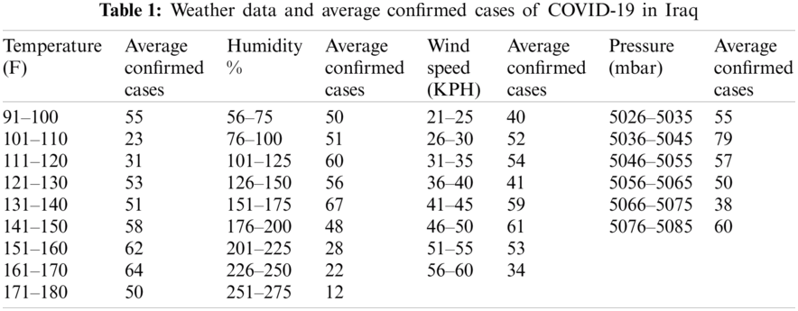
In Tab. 1, the transition probability matrix for the temperature is formulated as shown in Eq. (18);
For eigenspace decomposition of COVID-19 concerning the temperature, the model is constructed as Eq. (19);
Thus,
This is a homogenous system with infinitely many solutions. Using Microsoft Excel software, we obtain the solution as u1 = −0.2256, u2 = −0.3496, u3 = 0.2541, u4 = −1.2075, u5 = 0.8819, u6 = 0.7144, u7 = 0.8755, u8 = 2.798, and u9 = −0.3646.
4 Implementation of the Proposed Eigenspace Decomposition on the Transition Matrix of Humidity and COVID-19 Confirmed Cases in Iraq
The transition matrix based on Tab. 1 is constructed as shown in Eq. (22);
The eigenspace of the matrix Eq. (22) is formulated as Eq. (23).
Finally, from simplifications, we get Eq. (25);
The homogenous system Eq. (25) has infinitely many solutions. The Microsoft Excel solution of the system gives u1 = −1.3388, u2 = −0.8187, u3 = 1.3506, u4 = −0.5861, u5 = 0.2064, u6 = −0.1283, u7 = −2.3931, u8 = −4.9108, and u9 = 0.1039.
5 Implementation of the Proposed Eigenspace Decomposition on the Transition Matrix of Wind Speed and COVID-19 Confirmed Cases in Iraq
Using Tab. 1 and based on [31,38–40], we construct the transition matrix of the COVID-19 cases concerning the wind speed as shown in Eq. (26).
The eigenspace decomposition is presented in Eq. (27);
Computations give Eq. (29) such as
The Microsoft Excel software solution (29) yields u1 = 2.5387, u2 = −0.2497, u3 = −0.208, u4 = 0.01448, u5 = −0.8526, u6 = 1.846, u7 = −4.5585, and u8 = 0.5075.
6 Implementation of the Proposed Eigenspace on the Transition Matrix of Pressure and Confirmed Cases of COVID-19 in Iraq
The data shown in Tab. 1 are used to construct the transition matrix Eq. (30).
The eigenspace is presented as Eq. (31);
After the simplification, we get Eq. (33).
Solving with the Microsoft Excel software helps us obtain the solution as u1 = 0.07709, u2 = 0.04081, u3 = −0.1649, u4 = −0.7841, u5 = 0.8975, and u6 = −0.9336.
This section is dedicated to analyzing the results obtained from model Eqs. (21), (25), (29), and (33). The calculation results are shown in Tab. 2 and Figs. 1–4. The intensive analysis showed that COVID-19 has a cyclic attitude concerning temperature, humidity, wind speed, and pressure.
The dynamics of COVID-19 decrease at 130 F and show a minimum of approximately 120 F; after that, steady behavior is detected at approximately 160 F. It peaks at 170 F and then decreases; for details, see Fig. 1 and Tab. 2.
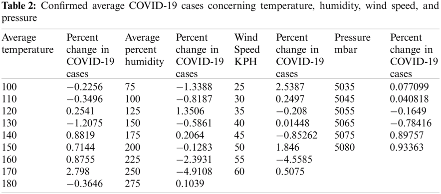
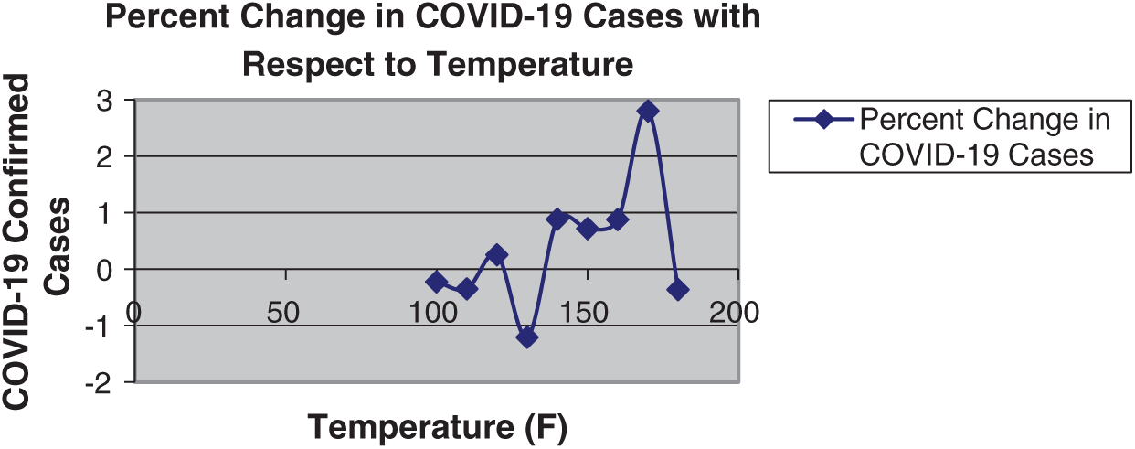
Figure 1: Percent change in COVID-19 cases concerning temperature
COVID-19 disease dynamics concerning humidity show cyclic behavior. The percent change in COVID-19 cases increases until a 125% humid climate. The cases then go until the bottom level is achieved under a 200% humid climate. The disease has slightly stable dynamics from 150% to 200% humidity as shown in Fig. 2 and Tab. 2.
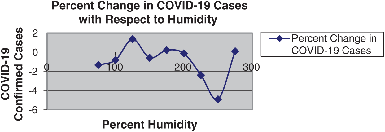
Figure 2: Percent change in COVID-19 cases concerning humidity
The most promising results of the disease are recorded concerning changes in wind speed. COVID-19 disease dynamics concerning wind speed show a decreasing trend until 45 KPH. The percent change in COVID-19 cases then increases to 50 KPH. The cases then go on to spread disease concerning wind speed until the bottom level is achieved at 55 KPH. This situation is shown in Fig. 3 and Tab. 2.
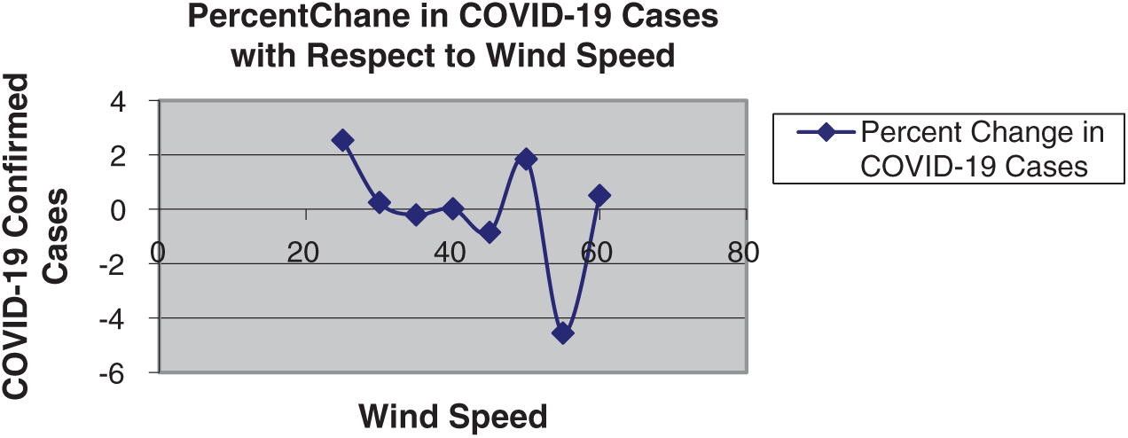
Figure 3: Percent change in COVID-19 cases concerning wind speed
The COVID-19 results for pressure show a stable trend until 5055 mbar pressure. The percent number of COVID-19 cases then decreases, touching a bottom level at 5065 mbar. Beyond this level, the percent change in COVID-19 confirmed cases for pressure increases, as shown in Fig. 4 and Tab. 2.
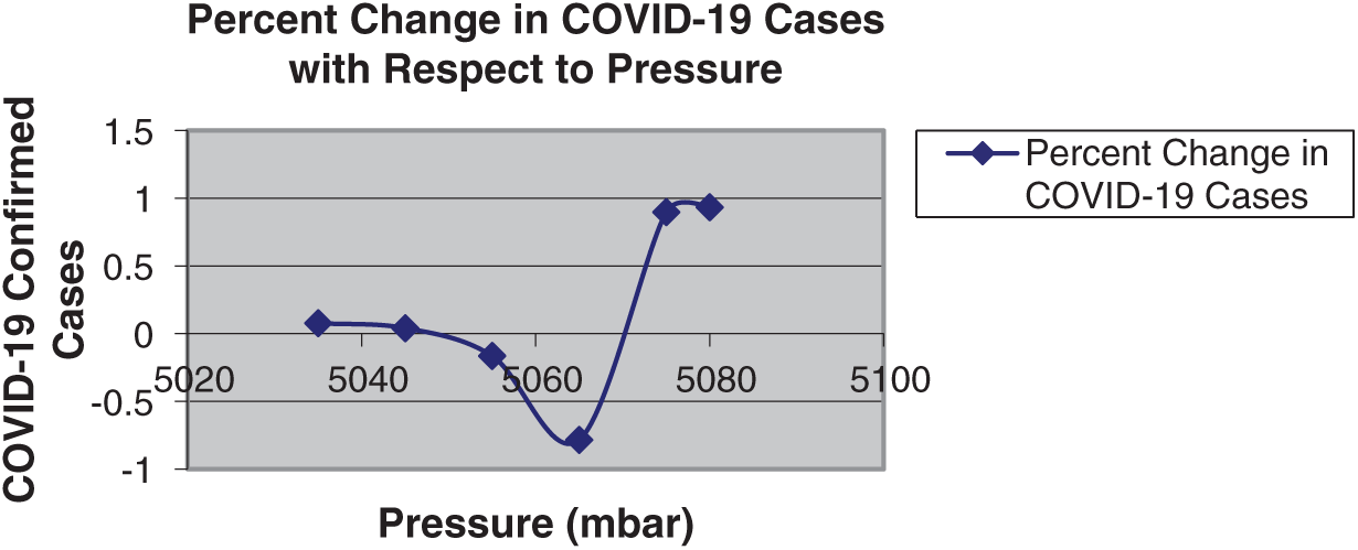
Figure 4: Percent change in COVID-19 cases concerning pressure
The spread of COVID-19 infection was reported to be lower in Iraq than in many Gulf countries, especially Iran and Saudi Arabia. We assume that this finding was due to the serious, strict measures taken by the government of Iraq. Some of the facts are as following:
1. The ban on international travel and immigrants.
2. The postponement of the religious gatherings.
3. Iraq imposed better quarantine and isolation and separation facilities on suspected and confirmed COVID-19 patients.
In this research, the weather effects on confirmed COVID-19 cases are studied. First, the eigenspace of the average numbers of COVID-19 cases concerning temperature, humidity, wind speed, and pressure are formulated and then solved. The transition matrix of change in COVID-19 concerning temperature is formulated. The eigenspace decomposition of COVID-19 infections concerning the change in the temperature is evaluated using the transition matrix that gives the long-run disease dynamics of temperature changes. This task is followed by formulating the transition matrix of the change in COVID-19 to the humidity level. The eigenspace decomposition of the change in COVID-19 infection to change in the humidity level is evaluated to give the long-run disease dynamics as a change in humidity level.
Furthermore, the transition matrix of change in COVID-19 concerning the wind speed is formulated. After formulation of the transition matrix, the eigenspace decomposition of COVID-19 infection to change in the wind speed is evaluated. Finally, the transition matrix of change in COVID-19 to pressure is formulated; its eigenspace decomposition is evaluated, giving the long-run disease dynamics as a change in atmospheric pressure.
Analysis of the results showed that the average numbers of confirmed COVID-19 cases have cyclic trends in temperature, humidity, wind speed, and atmospheric pressure. The results are visualized in the figures to show the change in the dynamics of COVID-19.
The analysis of our findings showed that the dynamic behavior of COVID-19 decreases at a temperature of 130 F. The minimum point of the spread occurred at 120 F, while a steady trend was reported at 160 F. The spread of the virus showed a peak when it reached 170 F. Moreover, considering the humidity figures, we noticed that COVID-19 infections increased until a 125% humid climate. The cases then decreased to a minimum point under a 200% humid climate, while slightly stable dynamics were seen at 150% to 200% humidity. A comprehensive analysis of the figures and results concerning the behavioral dynamics of COVID-19 regarding the wind speed shows a decreasing trend until 45 KPH. The change in COVID-19 cases then increases to 50 KPH. After that, the spread decreases to a bottom level at 55 KPH. In the end, the visual and analytical results concerning changes in COVID-19 show a stable trend in atmospheric pressure until 5055 mbar. The number of COVID-19 cases then decreases when this pressure reaches 5065 mbar.
Acknowledgement: This research was funded by the Deanship of Scientific Research at Princess Nourah Bint Abdulrahman University through the Fast-track Research Funding Program.
Funding Statement: The authors received no specific funding for this study.
Conflicts of Interest: The authors declare that they have no conflicts of interest to report regarding the present study.
1. Z. Wang, J. Wang and J. He, “Active and effective measures for the care of patients with cancer during the COVID-19 spread in China,” JAMA Oncology, vol. 6, no. 5, pp. 631–632, 2017. [Google Scholar]
2. H. Chen, J. Guo, C. Wang, F. Luo, X. Yu et al., “Clinical characteristics and intrauterine vertical transmission potential of COVID-19 infection in nine pregnant women: A retrospective review of medical records,” The Lancet, vol. 395, no. 2020, pp. 809–815, 2020. [Google Scholar]
3. Z. Xu, L. Shi, Y. Wang, J. Zhang, L. Huang et al., “Pathological findings of COVID-19 associated with acute respiratory distress syndrome,” The Lancet Respiratory Medicine, vol. 8, no. 4, pp. 420–422, 2020. [Google Scholar]
4. T. Ai, Z. Yang, H. Hou, C. Zhan, C. Chen et al., “Correlation of chest CT and RT-PCR testing coronavirus disease 2019 (COVID-19) in China: A report of 1014 cases,” Radiology, vol. 296, no. 2, pp. 32–40, 2020. [Google Scholar]
5. X. Chen, Y. Yang, M. Huang and Y. Wan, “Differences between COVID-19 and suspected then confirmed SARS-CoV-2-negative pneumonia: A retrospective study from a single-center,” Journal of Medical Virology, vol. 92, no. 9, pp. 1572–1579, 2002. [Google Scholar]
6. WHO, Coronavirus Disease 2019 (COVID-19Situation Report-69. Geneva, Switzerland: World Health Organization, 2020. [Google Scholar]
7. J. Gao, Z. Tian and X. Yang, “Breakthrough: Chloroquine phosphate has shown apparent efficacy in the treatment of COVID-19 associated pneumonia in clinical studies,” Bioscience Trends, vol. 14, no. 1, pp. 72–73, 2020. [Google Scholar]
8. M. Lipsitch, D. L. Swerdlow and L. Finelli, “Defining the epidemiology of Covid-19 studies needed,” New England Journal of Medicine, vol. 382, no. 2020, pp. 1194–1196, 2020. [Google Scholar]
9. F. Zhou, T. Yu, R. Du, G. Fan, Y. Liu et al., “Clinical course and risk factors for mortality of adult inpatients with COVID-19 in Wuhan, China: A retrospective cohort study,” The Lancet, vol. 395, no. 10229, pp. 1054–1062, 2020. [Google Scholar]
10. S. Lee, G. Chowell and C. Castillo-Chávez, “Optimal control for pandemic influenza: The role of limited antiviral treatment and isolation,” Journal of Theoretical Biology, vol. 265, no. 2, pp. 136–150, 2010. [Google Scholar]
11. E. Hansen and T. Day, “Optimal control of epidemics with limited resources,” Journal of Mathematical Biology, vol. 62, no. 3, pp. 423–451, 2011. [Google Scholar]
12. A. R. Tuite, J. Tien, M. Eisenberg, D. J. D. Earn, J. Ma et al., “Cholera epidemic in Haiti-2010: Using a transmission model to explain the spatial spread of disease and identify optimal control interventions,” Annals of Internal Medicine, vol. 154, no. 9, pp. 593–601, 2011. [Google Scholar]
13. H. S. Rodrigues, M. T. Monteiro and D. F. Torres, “Vaccination models and optimal control strategies to dengue,” Mathematical Biosciences, vol. 247, no. 2014, pp. 1–12, 2014. [Google Scholar]
14. P. Rodrigues, C. J. Silva and D. F. Torres, “Cost-effectiveness analysis of optimal control measures for tuberculosis,” Bulletin of Mathematical Biology, vol. 76, no. 10, pp. 2627–2645, 2014. [Google Scholar]
15. D. P. Moualeu, M. Weiser, R. Ehrig and P. Deuflhard, “Optimal control for a tuberculosis model with undetected cases in Cameroon,” Communications in Nonlinear Science and Numerical Simulation, vol. 20, no. 3, pp. 986–1003, 2015. [Google Scholar]
16. L. L. Pang, S. Ruan, S. Liu, Z. Zhao and X. Zhang, “Transmission dynamics and optimal control of measles epidemics,” Applied Mathematics and Computation, vol. 256, no. 2015, pp. 131–147, 2015. [Google Scholar]
17. A. Rachah and D. F. Torres, “Mathematical modeling, simulation, and optimal control of the 2014 ebola outbreak in West Africa,” Discrete Dynamics in Nature and Society, vol. 2015, no. 842792, pp. 1–10, 2015. [Google Scholar]
18. A. Rachah and D. F. Torres, “Dynamics and optimal control of Ebola transmission,” Mathematics in Computer Sciences, vol. 10, no. 3, pp. 331–342, 2016. [Google Scholar]
19. D. P. Gao and N. J. Huang, “Optimal control analysis of a tuberculosis model,” Applied Mathematical Modeling, vol. 58, no. 2017, pp. 47–64, 2017. [Google Scholar]
20. B. Kolman and D. R. Hill, Introductory Linear Algebra with Applications, 7th ed., Singapore: Pearson Education Inc, 2003. [Google Scholar]
21. M. S. Abdo, K. S. Hanan, A. W. Satish and K. Pancha, “On a comprehensive model of the novel coronavirus (COVID-19) Mittag–Leffler derivative,” Chaos, Solitons & Fractals, vol. 135, no. 109867, pp. 1–14, 2020. [Google Scholar]
22. R. U. Din, K. Shah, I. Ahmad and T. Abdeljawad, “Study of transmission dynamics of novel COVID-19 by using mathematical model,” Advances in Difference Equations, vol. 2020, no. 323, pp. 1–13, 2020. [Google Scholar]
23. A. Zeb, E. Alzahrani, V. S. Erturk and G. Zaman, “Mathematical model for coronavirus disease 2019 (COVID-19) containing isolation class,” BioMed Research International, vol. 2020, no. 3452402, pp. 1–7, 2020. [Google Scholar]
24. Z. Zhang, “A novel covid-19 mathematical model with fractional derivatives: Singular and non-singular kernels,” Chaos, Solitons & Fractals, vol. 139, no. 110060, pp. 1–11, 2020. [Google Scholar]
25. M. A. Khan and A. Atangana, “Modeling the dynamics of novel coronavirus (2019-nCov) with fractional derivative,” Alexandria Engineering Journal, vol. 2, no. 33, pp. 1–11, 2020. [Google Scholar]
26. K. Shah, T. Abdeljawad, I. Mahariq and F. Jerad, “Quantitative analysis of a mathematical model in the time of COVID-19,” BioMed Research International, vol. 2020, no. 5098598, pp. 1–11, 2020. [Google Scholar]
27. M. S. Abdo, K. Shah, H. A. Wahash and S. K. Panchal, “On a comprehensive model of the novel coronavirus (COVID-19) under Mittag–Leffler derivative,” Chaos, Soliton and Fractals, vol. 135, no. 109867, pp. 1–14, 2020. [Google Scholar]
28. M. Yousef, S. Zamir, M. Riaz, S. M. Hussain and K. Shah, “Statistical analysis of forecasting COVID-19 for upcoming month in Pakistan,” Chaos, Soliton and Fractals, vol. 138, no. 109926, pp. 1–14, 2020. [Google Scholar]
29. S. Ahmad, A. Ullah, Q. M. Al-Mdallah, H. Khan, K. Shah et al., “Fractional order mathematical modeling of COVID-19 transmission,” Chaos, Soliton and Fractals, vol. 139, no. 110256, pp. 1–5, 2020. [Google Scholar]
30. R. U. Din, K. Shah, I. Ahmad and T. Abdeljawad, “Study of transmission dynamics of novel COVID-19 by using mathematical model,” Advances in Difference Eqations, vol. 2020, no. 323, pp. 1–13, 2020. [Google Scholar]
31. M. Arfan, K. Shah, T. Abdeljawad, N. Mlaiki and A. Ullah, “A Caputo power law model predicting the spread of the COVID-19 outbreak in Pakistan,” Alexandria Engineering Journal, vol. 60, no. 1, pp. 447–456, 2021. [Google Scholar]
32. D. Baleanu, H. Muhammadi and S. Rezapour, “A fractional differential equation model for the COVID-19 transmission by using the Caputo–Fabrizio derivative,” Advances in Difference Equations, vol. 2020, pp. 299, 2020. [Google Scholar]
33. W. Gao, P. Veeresha, D. G. Prakasha and H. M. Baskonus, “Novel dynamical structures of 2019-nCoV with nonlocal operator via powerful computational technique,” Biology, vol. 9, no. 5, pp. 107, 2020. [Google Scholar]
34. D. Baleanu, H. Muhammadi and S. Rezapour, “Analysis of the model of HIV-1 infection of CD4+ T-cell with a new approach of fractional derivative,” Advances in Difference Equations, vol. 2020, no. 71, pp. 327, 2020. [Google Scholar]
35. W. Gao, P. Veeresha, H. M. Baskonus, D. G. Prakasha and P. Kumar, “A New Study of unreported Cases of 2019-nCOV epidemic outbreaks,” Chaos, Solitons and Fractals, vol. 138, no. 554, pp. 109929, 2020. [Google Scholar]
36. W. Gao, H. M. Baskonus and L. Shi, “New investigation of Bats–Hosts reservoir-people coronavirus model and apply to 2019-nCoV system,” Advances in Difference Equations, vol. 2020, no. 1, pp. 391, 2020. [Google Scholar]
37. S. Kumar, A. Ahmadian, R. Kumar, D. Kumar, J. Singh et al., “An efficient numerical method for fractional SIR epidemic model of infectious disease by using Bernstein wavelets,” Mathematics, vol. 8, no. 4, pp. 558, 2020. [Google Scholar]
38. Time and Date, “Past weather in Baghdad-April 2020,” 2020. [Online]. Available: https://www.timeanddate.com/weather/iraq/baghdad/historic?month = 4&year = 2020. [Google Scholar]
39. The World Health Organization, WHO Hands Over Essential Health Commodities to the Ministry of Health to Contain COVID-19 in Iraq. New York, United States: OCHA Services, 2020. [Google Scholar]
40. Worldometers, COVID-19 pandemic in Iraq-April. Geneva, Switzerland: The World Health Organization, 2020. [Google Scholar]
 | This work is licensed under a Creative Commons Attribution 4.0 International License, which permits unrestricted use, distribution, and reproduction in any medium, provided the original work is properly cited. |