Computers, Materials & Continua DOI:10.32604/cmc.2021.017700
Article

Mango Leaf Disease Identification Using Fully Resolution Convolutional Network

Rabia Saleem1, Jamal Hussain Shah1,*, Muhammad Sharif1 and Ghulam Jillani Ansari2

1COMSATS University Islamabad, Wah Campus, 47040, Pakistan
2University of Education, Lahore, 54000, Pakistan
*Corresponding Author: Jamal Hussain Shah. Email: jamalhussainshah@gmail.com
Received: 08 February 2021; Accepted: 01 May 2021

Abstract: Due to the high demand for mango and being the king of all fruits, it is the need of the hour to curb its diseases to fetch high returns. Automatic leaf disease segmentation and identification are still a challenge due to variations in symptoms. Accurate segmentation of the disease is the key prerequisite for any computer-aided system to recognize the diseases, i.e., Anthracnose, apical-necrosis, etc., of a mango plant leaf. To solve this issue, we proposed a CNN based Fully-convolutional-network (FrCNnet) model for the segmentation of the diseased part of the mango leaf. The proposed FrCNnet directly learns the features of each pixel of the input data after applying some preprocessing techniques. We evaluated the proposed FrCNnet on the real-time dataset provided by the mango research institute, Multan, Pakistan. To evaluate the proposed model results, we compared the segmentation performance with the available state-of-the-art models, i.e., Vgg16, Vgg-19, and Unet. Furthermore, the proposed model's segmentation accuracy is 99.2% with a false negative rate (FNR) of 0.8%, which is much higher than the other models. We have concluded that by using a FrCNnet, the input image could learn better features that are more prominent and much specific, resulting in an improved and better segmentation performance and diseases’ identification. Accordingly, an automated approach helps pathologists and mango growers detect and identify those diseases.

Keywords: Mango plant leaf; disease detection; CNN; FrCNnet; segmentation

1  Introduction

Plant diseases being insidious are becoming a nightmare for agricultural countries. Such diseases are causing colossal losses to the economies of countries by decreasing both the quantity and quality of fruit and field crops. Pakistan is one of those countries that earn precious foreign exchange by cultivating diverse crops, including fruits and vegetables. These crops are grown in various parts of the country. Therefore, the a need exist to employ image processing and computer vision research based smart techniques to identify the diseases. In recent times, researchers have been working hard to devise novel computer-based solutions for disease identification of mango plants at an early stage. That will help farmers protect their crop till it is harvested, resulting in reduction of economic losses [1]. Mango is the main popular fruit of Pakistan. Moreover, it is famous all over the world due to its distinct flavor, texture and nutritive value. Nowadays, the farmer of this area is worried about the effects of various diseases on mango plants, which is natural due to climate changes and other associated factors. Thus, it is imperative to protect this king of fruit plant to ensure the availability of a sweet and healthy mango for rest of the world. Unfortunately, few techniques exist to deal with fruit plants’ wellness, while it is only fateful that a small number of techniques have been reported till now to address mango plant diseases [2]. It's all due to the complex and complicated pattern of the diseased part on the leaf of the mango plant. Hence, to proceed in this resilient research area, efficient and robust techniques are required to cure mango plants. For doing this, the images were captured using the digital and mobile camera. These images are used as a baseline for identifying and detecting the disease on mango plant leaves. The visualization (detection and identification) of a disease is not an easy task. Mostly harmful diseases are found on the stems and leaves of the mango plant. To tackle all these issues and understand the leaf anatomy, there is much emphasis on precise identification of disease on leaves of the mango plant. Few common diseases on mango leaf have been described [3]. These common diseases include Blossom Blight, Anthracnose, and Apical Necrosis that are mostly found on the leaves of the mango plants.

Automated techniques play an important role in identifying and detecting the mango leaf diseases to handle such challenging issues. Few automated techniques such as segmentation and classification using K-means and Support-vector-machine (SVM) to detect the unhealthy region, respectively, are reported [4]. Further, a deep learning approach is employed to determine the type of mango [5] followed by a semantic segmentation-based method for counting a number of mangoes on the plant in the orchard using CNN [6] and leaf disease identification of mango plant using deep learning [2]. Hence, as per the discussion mentioned above, it reflects a dire need for an innovative and efficient automated technique for the detection, identification, and classification of the disease on the leaves of the mango plant.

Keeping the perspective in mind, this article is focused on the following issues to be covered: (1) image noise removal, which encounters due to camera adjustment and environment, (2) track change in disease shape, color, size, and texture, (3) tackle variation in the background and disease spot, (4) proper and accurate segmentation of diseased spot due to its similarity with the healthy parts of the leaf, (5) robust and useful feature extraction and fusion for classification at the later stage. The following key contributions of the intended work are listed below:

(i)   Low-contrast-haze-reduction (LCHR) approach is extended for enhancing and reducing the noise of infected regions in the query images.

(ii)   A method for segmentation based on deep learning is proposed for leaf disease detection. Compared with the latest available deep-learning models (Vgg-16, Vgg-19, and Unet) is performed to authenticate the proposed model.

(iii)   Color, texture (LBP), and geometric features are extracted; canonical-correlation-analysis (CCA) based fusion of extracted features is performed. The neighborhood-Component-Analysis (NCA) technique is applied to select the best features. Ten different types of classifiers are then implemented for recognition/identification.

(iv)   A comparison is also performed with existing articles for mango disease. For the authenticity of the proposed system, the classification results are also computed from three different strategies.

The rest of the article has the following sections: Section 2 highlights the literature review, while Section 3 depicts the details of the proposed work. The experimentation and results are discussed in Section 4, whereas the whole paper is concluded in Section 5.

2  Literature Review

In recent times, there are various methods developed for plant leaf disease detection. These are broadly categorized into disease detection and classification methods. Most of the techniques use a deep convolution network for segmentation, feature extraction, and classification considering the images of mango, citrus, grapes, cucumber, wheat, rice tomato, and sugarcane. Likewise, these methods are also suitable for fruits and their leaf diseases. Since few diseases can be correctly identified if they are precisely segmented and relevant features are extracted for classification purposes. Machine learning techniques are generally used, such as disease symptom enhancement and segmentation support, to calculate texture, color, and geometric features. Further, these techniques are also helpful for the classification of the segmented disease symptom. As a result, all this could be applied to make an automated computer-based system work efficiently and robustly.

Iqbal et al. [7], in their presented survey, discussed different detection and classification techniques and concluded that all these were at an infancy stage. Not much work has been performed on plants, especially the mango plant. Further, in their survey paper, they have discussed almost all the methods considering their advantages, disadvantages, challenges, and concepts of image processing to detect disease.

Sharif et al. [8] have proposed an automated system for the segmentation and classification of citrus plant disease. They have adopted an optimized weighted technique to segment the diseased part of the leaf symptom in the first phase of the proposed system. Afterward, in the second phase, various descriptors, including color, texture, and geometric, are combined. Finally, the optimal features are selected using a hybrid feature selection method that consists of the PCA approach, entropy, and covariant vector based on skewness. As a result, the proposed system has achieved above 90% accuracy for all types of diseases. Few prominent articles regarding classification of wheat grain [9], apple grading based on CNN [10], crop characterization by CNN based target-scattering-model [11], plant leaf disease, and soil-moisture prediction by introducing support vector (SVM) for feature classification [12], and UAV-based smart farming for the classification of crop and weed reflecting the use of geometric features have been reported. Safdar et al. [13] applied watershed segmentation to segment the diseased part. The suggested technique is applied to the combination of three different citrus datasets. The outcome of their technique is 95.5% accuracy, which is incredible for segmenting the diseased part. Febrinanto et al. [14] used the K-nearest-neighbour approach for segmentation. The detection rate of their methodology is 90.83%. Further, the authors segment the diseased part of the citrus leaf using a two and nine clusters approach by incorporating optimal minimum bond parameters that are 3%, which lead to final accuracy of 99.17%.

Adeel et al. [15] achieved a 90% and 92% accuracy level for segmentation and classification, respectively, on grape images from the Plant Village dataset. Results were obtained by applying the local-contrast-haze-reduction (LCHR) enhancement technique and LAB color transformation to select the best channel for thresholding. After that, color, texture, and geometric features were extracted and fused by canonical correlation analysis (CCA). M-class SVM performs the classification of finally reduced features. Zhang et al. [16] presented a GoogLeNet and Cifar10 network to classify the diseases on maize leaves. The models presented by them achieved the highest accuracy when compared with VGG & Alexnet to classify nine different types of leaves of a maize plant. Gandhi et al. [17] worked on identifying plant leaf diseases using a mobile application. The authors presented their work with Generative Adversal Networks (GAN) to augment the images. Then classification was performed by using convolution neural networks (CNN) deployed in the smartphone application. Durmuş et al. [18] classified plant diseases of tomato plant leaf taken from the PlantVillage database. Two deep-learning architectures (Alex-net and squeeze-net) were tested, first Alex-Net and then Squeeze-Net. For both of these deep-learning networks, training and validation were done on the Nvidia Jetson TX1. Bhargava et al. [19] used different fruit images and grouped them into red, green, and blue for grading purposes. Then they subtracted the background using the split and merge algorithm. Afterward, they implemented four different classifiers viz. K-Nearest-Neighbor (KNN), Support-Vector-Machine (SVM), Sparse-Representative-Classifier (SRC), and Artificial-Neural-Network (ANN) to classify the quality. The maximum accuracy achieved for fruit detection using KNN was 80%, where K was taken as 10, SRC (85.51%), ANN (91.03%), and SVM (98.48%), respectively. Among all, SVM proved to be more effective in quality evaluation, and the results obtained were encouraging and comparable with the state-of-art techniques. Singh et al. [20] proposed a classification method considering infected leaves of the Anthracnose disease on the mango plants. They used a multilayer convolution neural network for this purpose. The technique was implemented on 1070 self-collected images. The multilayer-convolution-neural-network (MCNN) was developed for the classification of the mango plant leaves. As a result of this setup, the classification accuracy raised to 97.13% accurately. Kestur et al. [6] proposed a deep learning segmentation technique called Mangonet in 2019. The accuracy level of 73.6% was achieved using this method. Arivazhagan et al. [2] used a convolutional neural network (CNN) and achieved an accuracy of 96.6% for mango plant leaf images. In the mentioned technique, only feature extraction with no preprocessing was done.

Keeping in view the scanty literature, we proposed a precise deep-learning approach for the segmentation of the diseased leaves of the mango plant called a full resolution convolutional network (FrCNnet). We aim to extend the U-net deep learning model, which is a famous segmentation deep learning technique. This method directly segments the diseased part of the leaf after implementing some preprocessing.

This paper proposed a novel, precise deep learning approach for segmenting and classification of mango plant leaves. After segmenting the diseased part, three features (color, texture, and geometric) are extracted for fusion and classification purposes. The fused feature vector is then reduced using the PCA-based feature selection approach to obtain an optimal feature set to get enhanced classification accuracy. The dataset used for this work is a collection of self-collected images captured using different types of image capturing gadgets. The subsequent section will highlight in detail the work done in this regard.

3  Proposed Work

The first and foremost task for this work is preparing a dataset, a collection of RGB images gathered from various mango-producing areas of Pakistan, including Multan, Faisalabad, and Lahore. The collected images reflected dissimilar sizes, so the same was resized to 256×256 after getting annotated by the expert plant pathologists. The workflow of the proposed technique is shown in Fig. 1. The major steps of the proposed technique are: 1) preprocessing of images that consist of image resizing and contrast enhancement/stretching followed by data augmentation and ground-truth generation. 2) use of fine-tuned proposed FrCNnet to segmentation the resultant enhanced image using deep learning-based proposed model (codebook). 3) Color, texture, and geometric feature extraction, fusion, and PCA-based feature reduction applied before feature fusion. Finally, classification is applied by using ten classifiers.

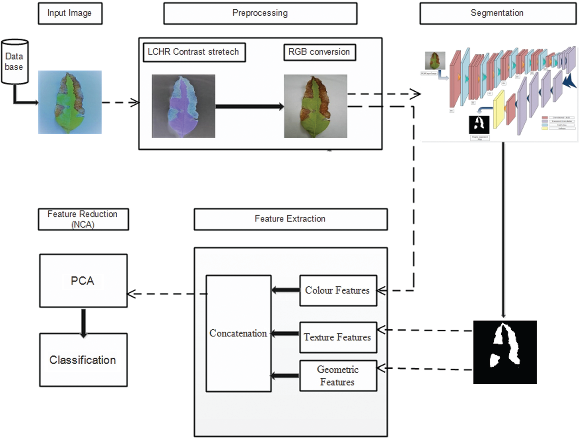
Figure 1: Framework diagram of basic concept and structure of a proposed automated system

3.1 Preprocessing

Preprocessing is an initial step adopted for this work. The purpose is to enhance image quality, which will help get better segmentation and classification accuracy. A detailed description of each step adopted in this regard is given below:

3.1.1 Resizing and Data Augmentation

We had a collection of 2286 images of the diseased mango leaves. Few of the images i.e., 2.88% (66 out of 2286), were distorted after resizing operation. These distorted images were discarded. It is well known that deep learning architectures are data-hungry algorithms. Hence, these algorithms require a large number of images to obtain the proper results. Thus, keeping in view the nature of deep learning architecture, 2220 images were then augmented by rotating and flipping them in horizontal, vertical, horizontal, plus vertical using the power law transformation with gamma = 0.5 and c = 1. By doing this, we had 8880 images available for training deep learning algorithms. Tab. 1 shows the distribution of the images of the dataset.

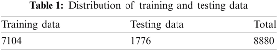
The images from 1 to 7104 and 7105 to 8880 were allocated for training and testing, respectively. Also, an equal image size of 256×256 was employed for the current study. Only diseased images were used for segmentation from the whole dataset, and 4440 rest of the healthy images were used for classification.

3.1.2 LCHR Contrast Stretching

The image quality matters a lot for further performance of the system in image processing techniques [21]. This approach helped reduce the errors affecting the system's performance in terms of its accuracy and execution cost. It could be done by removing noise from the image since noise can betray the system to detect the region of interest falsely. Moreover, the purpose of the image enhancement is useful for extracting different types of features used for the classification process. So, in this paper, we have extended Local-Contrast-Haze-Reduction (LCHR) approach [15], which helps solve few major issues such as 1) noise removal, 2) background correction, 3) regularization of image intensity and, 4) differentiation between diseased and healthy regions.

Suppose I(r,s) is the original input RGB image with the dimensions 256×256. The idea is to perform and improve the local contrast of the diseased area of the input images using nxm window size and given as follows.

J=β⋅μσ(1)

where β denotes the contrast parameter having values between 0 and 1. Global mean is denoted by μ and σ is the standard deviation. To obtain the final enhanced function, the local minima is computed denoted by M. The definitions for local minima (M) and standard deviation (σ) are as under.

M(I)=1n×n∑rn−1∑s=0n−1I(r,s)(2)

M(I)=1n×n∑rn−1∑s=0n−1(I(r,s)−M(I))2(3)

Further the contrast function (F) used these aforementioned computed values of local minima M and standard deviation σ. Hence, the formula for the contrast function becomes as:

F(I)=J×(I−M)+Mσ, where I∈(r,s)(4)

To conclude this step, the simple probability theory is used to perform the complement local contrast enhanced image F(I). Since, the image and its complement are equal to 1 as given under:

C(I)=1−P(F(I))(5)

where complement of the image is denoted by C(I) as shown in Eq. (5). In this way, we have regenerated an existing haze reduction technique [22], that helps to clear the diseased regions by removing the noise. The complete illustration of this section is shown in Fig. 2.

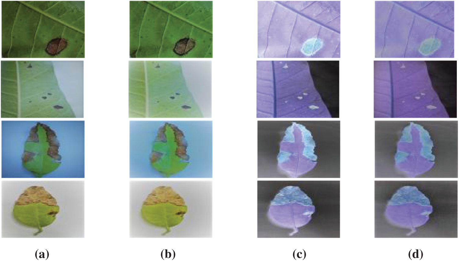
Figure 2: Different steps of LCHR contrast stretching (a) input image (b) contrast-enhanced image (c) complement of an image (d) haze reduction image

Afterward, a method was designed to generate the ground truth masks for the diseased leaves. The ground truth segmentation mask was only provided for the testing and training purpose to calculate matching the segmented image. Fig. 3 reflects the images and their ground truth masks.

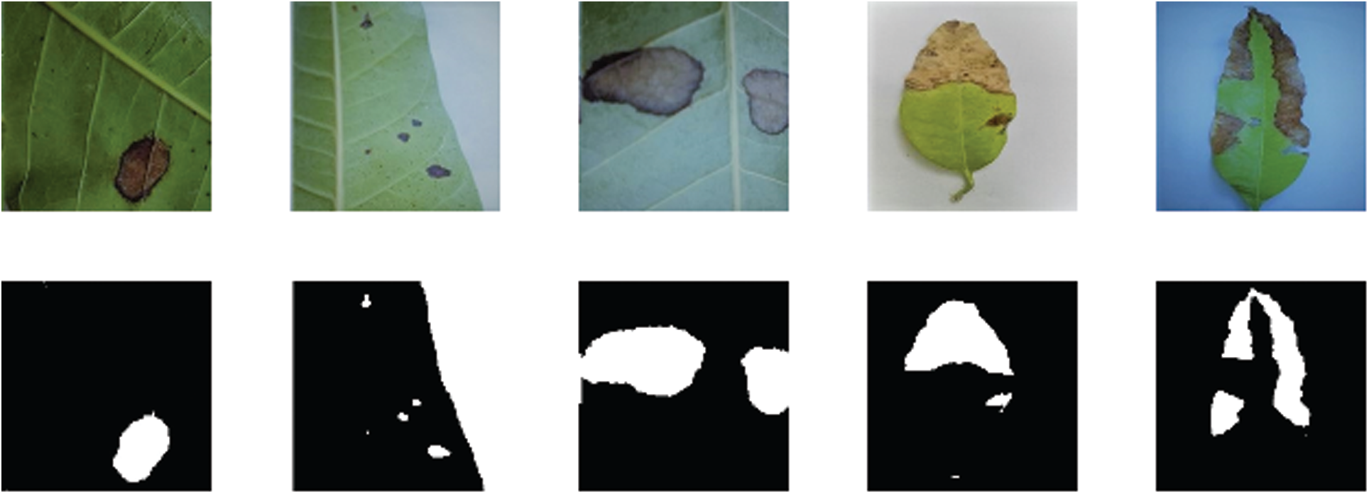
Figure 3: Images with their ground truth masks

3.2 Proposed FrCNnet Architecture/Model

To get pixel-wise classification from segmented images; generally, CNN is employed. The CNN has two important parts: 1) Convolutional layer and subsampling and 2) Upsampling.

The convolutional layer is used to extract deep features by using different filters from the input image. Subsampling is used to reduce the size of the feature map extracted [23]. The redundancy of the feature map extracted is eliminated and computational time reduced [24,25] to avoid overfitting. This is all because of the fact that reduced features represent the label of the input image. Subsampling reduces the resolution of the spatial features of an input image for the pixel-wise segmentation.

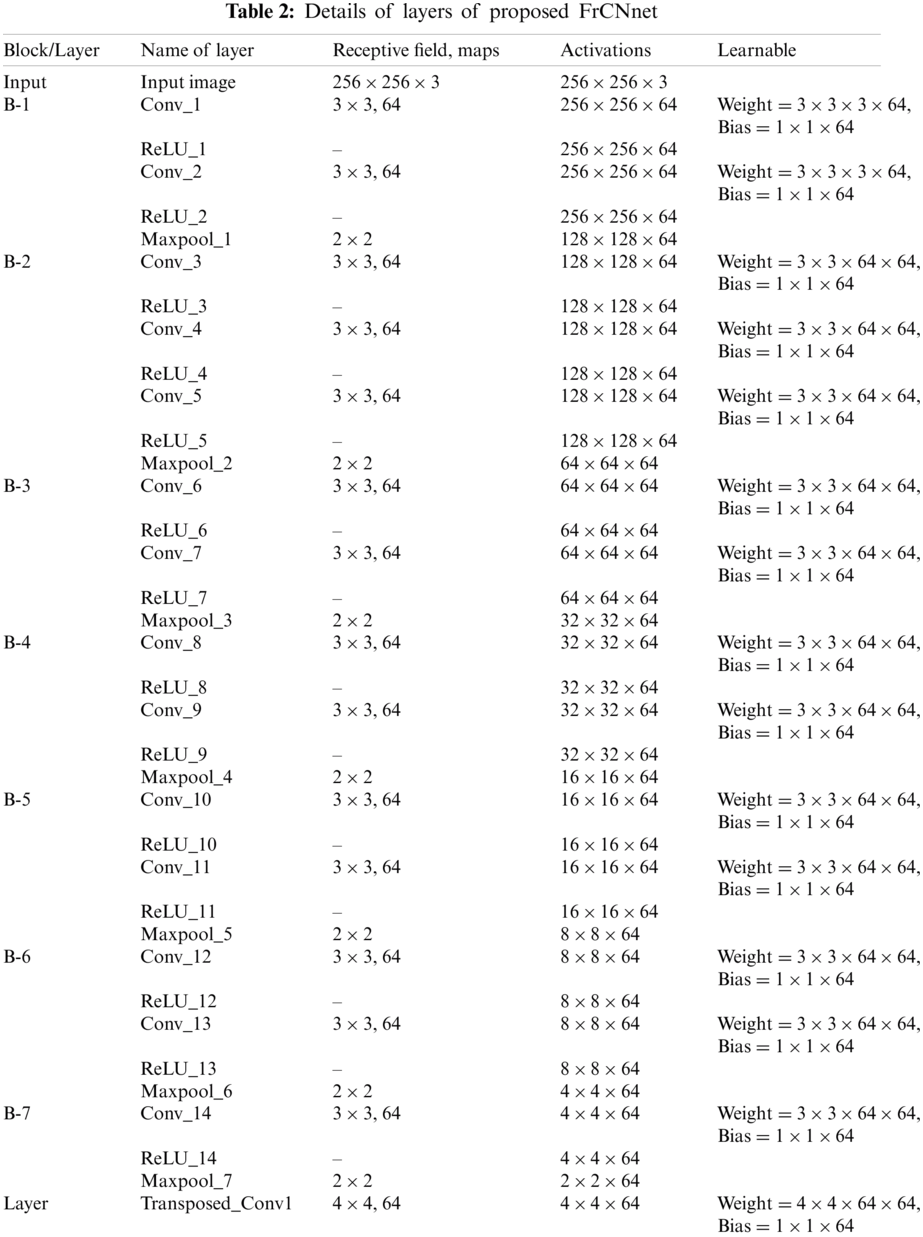
In the upsampling of the second part of the convolutional-neural-network, we have proposed a novel deep-learning-based segmentation method named as FrCNnet. This novel idea helps to eliminate concatenation operation from the architecture. In this way, full-resolution features of the input pixels are reserved. Here we adopt, transposed convolution which is an up-sampling technique that expands the size of images by doing some padding on the original image after the convolution operation (Convolutional layer). Every pixel can be represented as a training sample in this case. This proposed method consists of 51 layers inspired by Unet model [26] that has more layers then the proposed model for deep segmentation. It is customization in the layers of the Unet model in which concatenation operation is not used in proposed FrCNnet as it is used in Unet. Tab. 2 shows the details of each layer of the proposed system.

The CNN originally translated feature maps F using convolution operations [27,28]. The basic component of this network is ‘*’ called convolution operator, W(the filter-kernels) and φ(⋅) activation function. Therefore, the Nth feature map of layers (L) can be calculated as:

FLN=φ(WLN∗FL−1N+bLN)(6)

where bLN is a bias for each feature map generated by each layer. After each convolution operation we applied a non-linear activation-function via rectified-linear-units (ReLUs). The activation function ReLU is used due to its efficiency and robustness and counter the vanishing gradient problem instead of tan and sigmoid function described in [29] and [30]. ReLU can be defined as:

φ(x)=M(O,X)={X,if X≥0O,if X≤0(7)

The max-pooling operation in deep learning is used to resolve the over-fitting problem of deep layers. After the convolutional layer 2, 5, 7, 9, 11, 13, and 14 max-pooling function is used in the proposed architecture (FrCNnet) as shown in Tab. 2 reflects the dimensions of this operation. The purpose of using max-pooling is to downsample the input, including the image, output matrix, or hidden layer, by reducing the dimensions of the matrix. It also allows making assumptions about the features contained in the binned region. After that, the transposed-convolutional layers are used to increase or expand the size of the image. This is done by implementing certain padding techniques after the application of the convolutional layer. Softmax is the classifier (multinomial logistic regression), and it is the last and final layer of the proposed FrCNnet architecture. As a result of this, resolution of the output maps is the same as the input maps. Then the overall cross-entropy-loss function (class output layer or the pixel-classification layer) is calculated between ground truth (Z) and predicted segmented map (Z∧) to minimize the overall loss L of each pixel throughout the training. The pixel classification layer automatically ignores the pixel lables undefined during training and outputs of the categorical label for each image pixel processed by the network.

L=−(Zlog⁡(Z)+(1−Z)log⁡(1−Z))(8)

The aforementioned cross-entropy-loss function is used when a deep-convolution network is applied for a pixel-wise classification [31]. The objective of training through deep-learning models is to optimize the weight parameters at every layer—the optimization of single-cycle proceeds [32]. Firstly, the forward propagation is done sequentially to take the output at each layer. Secondly, by using the loss function error between the ground truth and predicted output, the accuracy is measured in the last layer of the output for the dataset. Thirdly, the back propagation is performed to minimize error in training dataset. As a result of all these, the training weights of the proposed architecture can be updated using the training data.

3.2.1 Feature Extraction and Fusion

Feature extraction is a very useful technique for machine learning and computer vision. Providing useful and efficient information and avoid redundancy are the major concerns of feature classification. For recognition of disease on plant leaves, texture and color features are more useful descriptors. The texture feature represents the texture analysis, and the color feature shows the color information of the diseased part. We have also extracted geometric, LBP, and color features to conduct a classification of diseases on the leaves of the mango. Feature extraction, fusion, and classification framework structure are shown in Fig. 4.

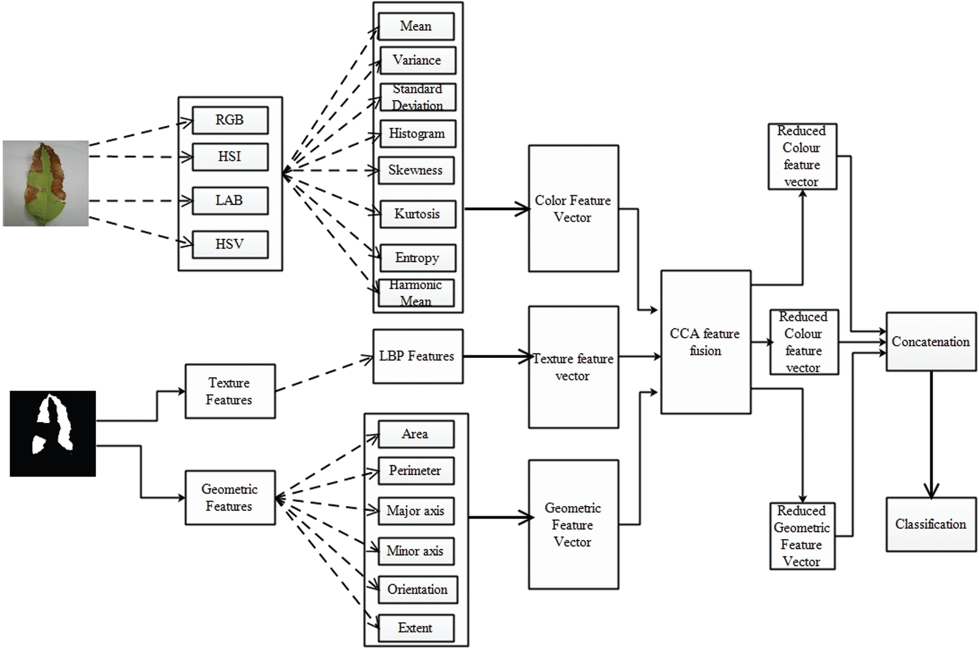
Figure 4: Framework of feature extraction, fusion and classification

The detailed description of each phase is as follows: in the training phase, the LCHR enhanced images are passed through the FrCNnet, and then the segmented map is broken for feature extraction and for calculating LBP and geometric features, the LCHR enhanced images are converted into gray-scale images; then the features are extracted as shown in Fig. 4.

After extracting the features, the Canonical Correlation Analysis (CCA) is used to fuse them into a single matrix. Moreover, a reduction technique of Neighborhood Component Analysis (NCA) reduces about 50% of features, and those are then fed to SVM to train a model. At the later stages, LCHR contrast images are also supplied to the proposed system in the testing phase that extracts the features and segments in the diseased part. After that, the texture and geometric features are computed from the segmented map of the images, as shown in Fig. 4. Finally, the recognition in terms of appropriate labels is performed by matching the trained labels with the fused and reduced features.

Color Features: Color features highlight and assume an indispensable job for recognition and detection of the diseased piece of the plants and individuals as every disease has its own shading. Color-features have been extracted in this article for the recognition of the disease on the leaves of a mango plant as discussed that each disease has its own shading and pattern. The various types of color spaces including red, green and blue (RGB), hue, intensity and saturation (HIS), luminance, a, b components (LAB) and hue, saturation and variance (HSV) are applied on the images in the wake of upgrading or enhancing the image using the LCHR approach. Eight types of statistical metrics are utilized to extract each type of color features (divided into three separate channels). The statistical metrics are area, mean, entropy, standard deviation, variance, kurtosis, skewness and harmonic mean. These all are expressed from Eqs. (9)–(16), respectively. The dimension of the combined feature vector for all color spaces is computed as 1 × 108, where each color channel has dimension 1 × 9. Therefore, final size of color feature vector after concatenating all the feature in a single matrix is n×108, where n is the total number of images (training and testing) and is denoted by (CF).

The formulae for the statistical metrics are as under:

A¯=(∑ai)/n,(9)

V=1n∑i=1n(ai−a′)2,(10)

σ=1n∑i=1n(ai−a′)2(11)

HF=∑j=1imj,(12)

Skewness=1n∑i=1n(ai−a′)3(1n∑i=1n(ai−a′)2)32,(13)

KR=n∑i=1n(Ai−Aavg)4(∑i=1n(Ai−Aavg)2)2(14)

Entropy=∑i=1c−pilog2pi,(15)

HM=n∑i=1n1ai(16)

where, A¯ denotes mean-feature, V denotes variance-feature, σ denotes the standard-deviation feature, HF denotes the histogram-feature, Skewness denotes skewness-feature, KR denotes kurtosis-feature, and HM denotes harmonic-mean-feature, respectively.

Texture Features: The local structure and texture of any object are determined by a Local Binary Pattern (LBP) method. This method extracts information from the local patterns as compared to pixel levels. To handle the texture complication of an image, an old but simple approach, LBP, is used [33]. The definition of LBP is given as under:

LBPA,B=∑A=0A−1F(gA−gc)2A,F(x)={1if x≥0;0otherwise(17)

The obtained vector in LBP represented by ψ(LBP) is 1×59 and for all the images in the datasets is n×59.

Geometric Features: Geometric features or sometimes known as shape-features, are generally used to recognize objects. The significance of these features is to perceive the object for collecting geometric data including edges, lines, corners, spots (blobs) and folds (ridges). Six types of geometric features are used in this work and are numerically represented as follows in Eqs. (18)–(23):

A=∑i=1n∑j=1mA[i,j](18)

p=φ[2L+2W](19)

Ma=d+e(20)

M′a=(d+e)2−F2(21)

θ=arctan⁡(R−P+(R−P)2+Q2Q),(22)

E=Area(A)Area of bounding box(23)

A major axis by, minor axis by, where area is represented by A, perimeter is represented by M′a,θ for representing orientation and extent is represented by E. In the above Eqs. (18)–(23) d, e are the distances from the focus-point in an ellipse, F represents a distance between the focus-point, P, Q, R are parameters representing distances from the central-point, L represents the length and W represents width. The size of geometric-feature vector length is n×6 where n is the total number of images and is denoted by ψ(GV).

Feature Fusion and Reduction: In feature fusion, numerous features are combined into a single vector. The fusion process shows a lot of progress in the applications where pattern recognition is implemented because each feature has its characteristics and qualities. Combining all the features gives much-improved performance, but it expands the computation cost. Therefore, we used CCA for this purpose. CCA feature fusion is used to maximize the correlation. Aside from all the benefits of feature fusion, there exist numerous issues with it as well. An increase in computational time and the problem of dimensionality occur if the features fussed are not equally represented. When the features are combined in a single vector, there may arise a redundant information problem. Therefore, Neighborhood-Correlation-Analysis (NCA) based feature reduction is performed to remove the dimensionality and redundant information after implementing canonical-correlation-analysis (CCA) for features fusion in this work.

Suppose {di}i=1n∈Rs, {ei}i=1n∈Rt and {fi}i=1n∈Ru where s, t, u are the dimensions of sample space, and n denotes observation size. The main purpose of CCA is to find projection directories given as below:

xd∈Rs,xe∈Rt,xfRu(24)

Eq. (24) shows the correlation between xdTD, xeTE, xfTF color, texture, and geometric features that are to be fused, where D=[d1,d2,…,d], E=[e1,e2,…,en] and F=[f1,f2,…,fn] are sample matrices. Formally CCA can be solved as:

ρ=maxxdTxeCdefxf(xdTCddxd)(xeTCeexe)(xfTCffxf)(25)

where Cdef=DEFT defines covariance matrix between feature sets and Cdd=DDT,Cee=EET,Cff=FFT represents covariance within three feature sets. When the matrices within feature sets are non-singular then CCA can be obtained by computing generalized Eigen-problem, which is formulated as:

(CdefCff−1Cfde000CfdeCee−1Cefd000CefdCdd−1Cdfe)(xdxexf)=λ(xdxexf)(26)

Let Xd=[xd1,xd2,…,xa,m],Xe=[xe1,xe2,…,xe,m],Xf=[xf1,xf2,…,xf,m] denote 3 projection directories matrices. Where the vector pairs (xdi,xei,xfi)i=1m corresponds to the largest m generalized Eigen-value. Fused feature obtained from the 3 modalities is as under:

Z(i)=(XdTdXeTeXfTf)(27)

where, Z(i) denotes the fused vector. The fused vector is obtained after the maximum correlation between features viz. color, texture, and geometric, discarding the irrelevant information. In order to obtain final classification results, sometimes it is significant to remove the redundant information. Therefore, Neighborhood-Correlation-Analysis (NCA) reduction method eliminates redundant information and only selects the good or informative features. Selected features are fed to classifiers to obtain the classification results. The proposed labeled results are shown in the results section.

3.2.2 Training and Testing

In recent times, agricultural applications, especially mango plants, still suffer from the shortage of data. This is due to the complexity, cost of the collection process due to the plant's availability at limited places, and labeling cost during data acquisition [34]. Hence all these factors motivate us, and we have collected the data from different mango-producing areas of Pakistan to overcome this issue. We adopted two strategies: 1) data-augmentation and 2) transfer-learning [14,24–26,35]. None of the techniques has been proposed for segmentation using deep learning on the agriculture sector i.e., specially mango plant. We train our dataset the Vgg16, Vgg19, and Unet models compared to our proposed FrCNnet architecture to evaluate the results. We used the distribution of datasets to test and test the results, which is mentioned above in Tab. 1. The evaluation of the proposed network performance and optimization were taken out independently. We have adopted the most recent deep learning approach that is double-crossed validation scheme. This approach is more reliable and commonly used in contrast to the trial-and-error method. Finally, the segmented images were fed into the system for feature extraction, fusion, and reduction and then for classification. The computation time for the training data is about 18 h for 100 epochs with a batch size of 20. Moreover, the segmentation of a single leaf took about 7.5 s. To implement the whole algorithm and its experiments, we used a personal computer having the following specifications: Intel® Xeon® processor with CPU frequency {2.2 GHz} having 32 GB RAM and NVIDIA GPU GEForce GTx1080 and Matlab 2018(b) on windows 64-bit for coding the algorithm.

4  Results and Discussion

As a priority, the accuracy-based results of the proposed segmentation technique are produced first, and afterward the classification results as per the proposed technique are given by employing different benchmark classifiers. The detailed description of all the results is presented in the following section.

4.1 Segmentation Results

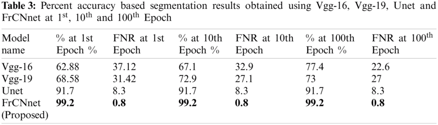
In this part, the proposed model's segmentation performance is discussed compared with the other state-of-the-art deep learning models. For acquiring segmentation results, the dataset is distributed in 7040 images for training and 1760 images for testing purpose; respectively, {Vgg-16}, Vgg-19, and Unet models were also implemented on this dataset to compare the results of the proposed model. These models were fine-tuned by using the same receptive fields, maps as in the proposed model. The quantitative results are arranged in tabular and also visualized the effect graphically. The matching accuracy of segmented part of the image with ground truth at 1st Epoch for Vgg-16 is 62.88%, for Vgg-19 is a bit higher than Vgg-16 that is 68.58%, for Unet model is 91.7%, much higher than Vgg-16 and Vgg-19 and the percentage for the proposed FrCNnet is 99.2% being much higher than Vgg-16 and Vgg-19 and Unet models. For the 10th Epoch, the accuracy of Vgg-16 is higher than at 1st epoch that is 67.1% and accuracy for Vgg-19 is also increased than at 1st epoch that is 72.9%, but it remains same for Unet at 1st and 10th epoch which is 91.7% and for proposed architecture FrCNnet it increases up to a highest level that is 99.2% same as on 1st epoch. Then the accuracies are checked for the 100th Epoch in which for Vgg-16, we have observed much increase up to 77.4%, a minimal increase in Vgg-19 at 100th Epoch; it becomes 73% at 100th epoch. We have seen an increase in accuracy for the Unet that is 91.7%. on proposed FrCNnet architecture and the accuracy percentage remained same as on 10th epoch but is greater than all the models that is found to be 99.2% shown in Tab. 3.

4.2 Classification

The proposed classification results are two folds: firstly, the classification results are performed for each disease-class with healthy-class. Secondly, classification is performed for all disease-classes including healthy-class. All these results are obtained using 10 cross folds that means the testing feature set is divided into 10 subsets out of which 1 subset is used for testing and 9 remaining folds are for training. This whole process is performed 10 times and an average value is calculated after ten iterations. For comparison purpose with proposed technique, 10 state of the art classifiers are selected including Linear discriminant, Linear-Support-Vector-Machine (LSVM), Quadratic-SVM (QSVM), Cubic-SVM, Fine KNN, Medium KNN, Cubic K-Nearest-Neighbor (CKNN), Weighted-KNN, Ensemble-Subspace-Discriminative (ESD) and Ensemble-subspace-KNN. The performance is measured using the parameters including sensitivity, specificity, AUC (Area Under the Curve), FNR (False Negative Rate), and accuracy. The detailed result analysis of the proposed system is presented in this section. The results are also presented in both graphical and tabular form.

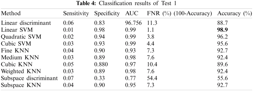
4.2.1 Test 1: Anthracnose vs. Healthy

In this test, classification of Anthracnose vs. healthy images was performed. We had 4440 images of Anthracnose diseased images with equal number of healthy images as well. Tab. 4 shows that accuracy of 98.9% is achieved by the Linear-SVM which is superior among all the other competitive classifiers. The values of other measures including Sensitivity, Specificity, Area Under the Curve (AUC), False Negative Rate (FNR) are 0.01, 0.98, 0.99, 1.1, respectively.

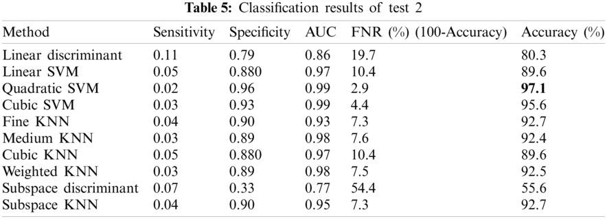
4.2.2 Test 2: Apical Necrosis vs. Healthy

In this test, classification of apical necrosis vs. healthy images was performed. We had 4440 images of Anthracnose diseased images with equal number of healthy images as well. Tab. 5 shows that accuracy of 97.1% is achieved by the Quadratic-SVM which is superior among all the other competitive classifiers. The values of other obtained measures including Sensitivity, Specificity, Area Under the Curve (AUC), False Negative Rate (FNR) are 0.02, 0.96, 0.99, 2.9, respectively.

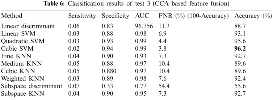
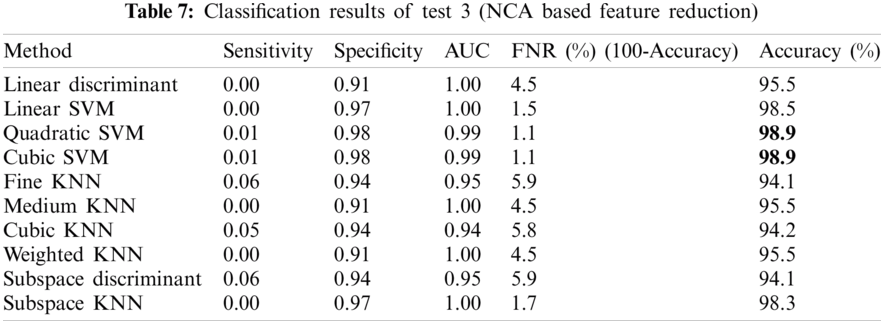
4.2.3 Test 3: All Diseases vs. Healthy

The results presented in this section are two folds: (i) CCA based features (color, texture and geometric) and (ii) NCA-based feature reduction. Tab. 6 shows the classification results obtained after CCA based feature fusion. The accuracy level of 96.2% is achieved by the Cubic-SVM which is superior among all the other competitive classifiers. The values of other measures including Sensitivity, Specificity, Area Under the Curve (AUC), False Negative Rate (FNR) are 0.02, 0.94, 0.99, 3.8, respectively.

Tab. 7 shows the classification results obtained after NCA based feature reduction. The accuracy of 98.8% is achieved by the Quadratic-SVM and Cubic-SVM is superior among all the other competitive classifiers. The values of other measures including Sensitivity, Specificity, Area Under the Curve (AUC), False Negative Rate (FNR) are 0.01, 0.98, 0.99, 1.1, 98.9, respectively for both the Quadratic-SVM and Cubic-SVM. This gives more accuracy as NCA based feature reduction removes redundant features provided by CCA based feature fusion.

4.3 Discussion

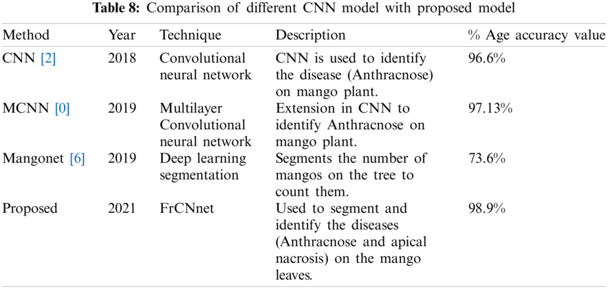
The obtained results are in conformity with the findings of Ramesh et al. (2019) who introduced a mango counter named Mangonet by using deep learning segmentation technique to attain the accuracy of 73.6%. Segmentation results of the proposed model are very much improved by 99.2% as compared to mangonet as shown in Tab. 8. Classification results obtained after feature extraction (color, texture and geometric) and NCA-based feature reduction are 98.9%, which are much improved than Arivazhagan et al., 2018 who obtained accuracy of 96.6% and Udhay et al., 2019 who presented Multilayer Convolutional neural network for the classification of mango leaves infected by anthracnose disease and his classification accuracy is 97.13%.

5  Conclusion

The technique FrCNnet was introduced in this paper that can be used to segment the diseased part so that it can be classified/identified timely and properly. We generated three types of ground truth masks to compare the results of the proposed model. The images were given to the system, and codebook (down-sampling (convolution, relu), up-sampling (deconvolution, relu), softmax, and pixel classification) layers were used in this work. Unlike the previous state-of-the-art deep learning approaches, FrCNnet can produce a full resolution feature of the input images. That leads to an improved segmentation performance. This limited-time is much feasible for the pathologists to practically segment the diseased leaf part—the results of the proposed model over-performed Vgg-16, Vgg-19, and Unet models. The results were evaluated on the images of the leaves of the mango plant provided by the mango research institute, Multan. In the future, a large number of the images are required to improve the segmentation performance of each class. Features are extracted, which are then fed into the classifiers to classify them after implementing CCA-based feature fusion and then NCA-based feature reduction. The classification accuracy achieved in this work by Quadratic SVM and Cubic SVM is 98.9% superior to the already available work.

Acknowledgement: We are thankful to Mango research institute, Multan and Tara Crop Sciences private limited for providing us the data (images).

Funding Statement: The authors received no specific funding for this study.

Conflicts of Interest: The authors declare that they have no conflicts of interest to report regarding the present study.

This work is licensed under a Creative Commons Attribution 4.0 International License, which permits unrestricted use, distribution, and reproduction in any medium, provided the original work is properly cited.