DOI:10.32604/cmc.2021.017364
| Computers, Materials & Continua DOI:10.32604/cmc.2021.017364 | |
| Article |
Cotton Leaf Diseases Recognition Using Deep Learning and Genetic Algorithm
1Department of Computer Science, HITEC University Taxila, Taxila, Pakistan
2Wah Engineering College, University of Wah, Wah Cantt, 47080, Pakistan
3College of Computer Engineering and Sciences, Prince Sattam Bin Abdulaziz University, Al-Khraj, Saudi Arabia
4Department of Computer Science and Engineering, Soonchunhyang University, Asan, Korea
5Faculty of Applied Computing and Technology, Noroff University College, Kristiansand, Norway
*Corresponding Author: Yunyoung Nam. Email: ynam@sch.ac.kr
Received: 28 January 2021; Accepted: 14 April 2021
Abstract: Globally, Pakistan ranks 4th in cotton production, 6th as an importer of raw cotton, and 3rd in cotton consumption. Nearly 10% of GDP and 55% of the country's foreign exchange earnings depend on cotton products. Approximately 1.5 million people in Pakistan are engaged in the cotton value chain. However, several diseases such as Mildew, Leaf Spot, and Soreshine affect cotton production. Manual diagnosis is not a good solution due to several factors such as high cost and unavailability of an expert. Therefore, it is essential to develop an automated technique that can accurately detect and recognize these diseases at their early stages. In this study, a new technique is proposed using deep learning architecture with serially fused features and the best feature selection. The proposed architecture consists of the following steps: (a) a self-collected dataset of cotton diseases is prepared and labeled by an expert; (b) data augmentation is performed on the collected dataset to increase the number of images for better training at the earlier step; (c) a pre-trained deep learning model named ResNet101 is employed and trained through a transfer learning approach; (d) features are computed from the third and fourth last layers and serially combined into one matrix; (e) a genetic algorithm is applied to the combined matrix to select the best points for further recognition. For final recognition, a Cubic SVM approach was utilized and validated on a prepared dataset. On the newly prepared dataset, the highest achieved accuracy was 98.8% using Cubic SVM, which shows the perfection of the proposed framework..
Keywords: Plants diseases; data augmentation; deep learning; features fusion; features selection
Globally, Pakistan ranks 4th in cotton production, 6th as an importer of raw cotton [1], and 3rd in cotton consumption. Nearly 10% of GDP and 55% of the country's foreign exchange earnings depend on cotton products [2]. Approximately 30%–40% of cotton is utilized for household consumption in the form of final products and the remaining is exported as raw material, clothes, and garments. The major areas in Pakistan where cotton grows are Rahim Yar Khan, Khanewal, Sahiwal, Layyah, D. G. Khan, Dadu, Khairpur, and Nawab Shah [3]. Farming along the Indus extends across nearly three million hectares, and the economy is strongly dependent on this cultivation. Approximately 1.5 million people in Pakistan are engaged in the cotton value chain.
Cottonseed oil meets almost 17.7% of the oil requirements in Pakistan [4]. In the textile industry, cotton has always been a popular crop for raw material [5], thus, it is imperative to properly deal with the crisis of cotton at the right time to save the textile industry [6]. The problem related to cotton can be a direct and significant cause of the crisis in the textile industry [7]. Leaves are the most essential part of the cotton plant, and almost 80%–90% of diseases are recognized from leaf appearance [8,9]. The annual cultivation of cotton uses over three million hectares, accounting for almost 14% of the country's cropped area. Plant diseases pose severe threat to important agricultural crops and plants [10]. Crops can be damaged and even wiped out entirely by these diseases [11]. Diseases and pests damage approximately 42% of the world's total agricultural crops annually. By selecting superior quality seeds and providing suitable environments for plants, farmers make efforts to improve crop production. However, naked eye identification of damage is not a successful approach, and farmers do not obtain authentic results. In addition, they have limited knowledge about cotton diseases, and in some cases, it is difficult to differentiate between different types of infections. Identifying crops’ diseases at the early stage is very important to save the crops [12]. According to experts, the most common approach to identify the diseases is the naked eye approach. This approach has many limitations, such as the requirement for continuous monitoring by experts, which may be expensive and time-consuming, particularly in vast farms and remote areas [13]. Using traditional approaches, it is almost impossible to identify diseases at an early stage with good accuracy and minimal computational time. Therefore, it is important to formulate methods of disease identification that can perform the task automatically, accurately, timely, and inexpensively [14,15].
Machine learning (ML) has become a fundamental part of the agricultural industry [16]. ML is derived from artificial intelligence [17] that allows computer applications to work precisely and accurately in finding the results. Algorithms used in ML are inspired by the characteristics of real-world objects [18]. The main aspects of such systems are that they learn mechanically and improve with repetition and experience [19]. The meaning of learning is to recognize and understand the input data and make intelligent decisions based on the given data. Nowadays, convolutional neural network (CNN) has become more popular than all other computer vision (CV) methods [20]. To perform different tasks, CNN requires training on large datasets. However, it is not easy to obtain high-dimensional data for learning by a CNN model in agriculture. Therefore, a transfer learning (TL) method was used. In this study, a subset of the most commonly occurring diseases was investigated, namely (i) Areolate Mildew, (ii) Myrothecium leaf spot, and (iii) Soreshine. A~few sample images are presented in Fig. 1.
A great revolution has emerged in the field of ML [21], CV [22], and robotics [23] after the invention of intelligence neural networks (NN) [24]. These systems are formulated by different arrangements of layers (convolution layer, pooling, and fully connected (FC)) and activation functions (ReLU, softmax, etc.) [25]. These NNs have some significant advantages:(i) An enormous number of variables can be handled simultaneously, (ii) improvement of two factors effectively, consistent, or discrete, (iii) they consider extensive testing of the cost surface; (iv) NN can optimize factors with very complex costs, and (v) they can achieve various ideal arrangements and not a solitary arrangement [26]. In [27] Edna evaluated and fine-tuned modern deep CNN by comparing different deep learning architectures, such as VGG [28] and ResNet. A total of 14 disease classes were considered in the presented work, collected from the Plant Village dataset. DenseNet [29] achieved a 99.75% accuracy score, higher than those of existing techniques. Qiufen et al. [30] utilized different CNN models for TL, such as AlexNet, GoogleNet, and ResNet, to identify diseases in a soybean leaf. In these models, the highest classification accuracy obtained by ResNet [31] was 93.71%. In [32] Shanwen proposed a new approach for the recognition of cucumber disease. The approach consisted of three pipelined procedures: the diseased leaf was segmented using K-means-based clustering, different types of features, such as shape features and color features, were extracted from laceration information, and then, using sparse representation, the diseased leaf images were classified. Many other techniques have been proposed in the literature for the identification and recognition of plant diseases. Most of these studies focused on the segmentation process, and few concentrated on the classification. For accurate classification, feature fusion and selection techniques were proposed [33]. Feature fusion is a process that extracts information from a group of training and testing images and integrates without any loss of data. After the fusion process, the resulting feature matrix is improved to make it more informative. Some researchers discussed that some irrelevant or redundant features are added to the fused matrix, which need to be discarded. To solve this type of problem, researchers introduced several feature selection techniques based on heuristic and meta-heuristic techniques.

Figure 1: Categories of cotton diseases used as a dataset
Researchers have developed different techniques to identify cotton leaf diseases; however, there are still many limitations, and a few of them are as follows: i) choice of color spaces, ii) weak contrast and boundaries, iii) similarities between infected and regular cotton leaves, iv) different symptoms with similar features and similar shapes, and v) selection of useful features for accurate recognition. In this study, we proposed a new automated approach for cotton leaf disease recognition using deep learning. The steps are as follows: a) a self-collected dataset of cotton diseases is prepared and labeled by an expert; b) data augmentation (DAg) is performed on the collected dataset to increase the number of images for better training; c) a pre-trained deep learning model named ResNet101 is employed and trained through TL; d) features are computed from the third and fourth last layers and serially combined into one matrix, and e) a genetic algorithm (GA) is applied to the combined matrix to select the best points for final recognition.
The rest of the manuscript is organized as follows. The proposed methodology, which includes deep learning model-based feature extraction and feature reduction, is discussed in Section 2. The results of the proposed method are discussed in Section 4. Finally, the conclusions drawn from this work are presented in Section 5.
In this study, ResNet101 was used along with TL to recognize cotton leaf diseases. In the first step, the dataset consisted of three major diseases in cotton leaves: Areolate Mildew, Myrothecium leaf spot, and Soreshine. The dataset used in this study was not sufficiently large. The DAg technique was applied to increase the size of the dataset. After performing DAg, the enhanced dataset was provided to ResNet101 for feature extraction. The training to testing ratios were set to 80/20, 70/30, and 50/50. Features were extracted from both layers (average pool and FC) and fused using a serial-based approach. To select the most prominent and non-redundant features, we applied a GA to the fused feature vector. The notable features selected by the GA were provided to Cubic SVM for final recognition. The main flowchart is shown in Fig. 2. The description of each step follows.

Figure 2: The proposed architecture of cotton leaf diseases recognition using deep learning
Because the dataset was limited in this study, we performed DAg. The total number of original images was 95, as shown in Fig. 1. Therefore, enhancement of the dataset was essential. For this purpose, the DAg technique was applied. First, images were rotated at different angles, such as 90°, 180°, and 270°. In addition to rotation, the flipping operation was also performed at different angles to increase the size of the actual dataset. Before DAg, there were only 30 images in each class, and after applying augmentation, 1000 images in each class were obtained.
2.2 Convolutional Neural Network
CNN is a famous deep neural network (DNN) model for feature extraction. The inputs of CNN are similar to those of the two-dimensional (2D) array. Similar to feed-forward NNs, neurons used in CNN also have learnable weights and biases. CNNs work directly on images rather than focusing on feature extraction. CNNs are beneficial for image classification and image recognition. Two main parts are included in the CNN: extraction of features and classification of features. The extraction of features depends on the activation function applied to specific layers, while the classification task represents the key class defined before the training process. The key strength of CNN is to extract the strong and complex features of an image and generate good results during the classification phase.
Convolution layer: After the input layer, the first layer of CNN is the convolution layer. The weights (original image pixels) are transformed through this layer and processed for the next layer. In this layer, more robust features are captured in the form of patches. The strongly correlated features are selected and then passed to the next layer for further processing based on each patch feature. The convolution operation is described below.
After every convolution operation, an additional operation is performed, known as the ReLU operation. The ReLU activation layer [34] is described as follows.
This equation explains that all negative values, after applying this function, are converted to zero. During the DNN training, each next layer's input comes from the previous layer's output. With time, the parameters of the previous layer changes. Therefore, the allocation of input data to the layers varies extensively. This requires lower learning rates, which slows down the training process. This internal problem can be solved through normalization called batch normalization (BN) [35]. Using this technique, the mean and variance are calculated and implemented in a new function, as given below.
where
where
Modified ResNet 101: ResNet is a deep residual network with very deep architectures. It creates a direct path to propagate information throughout the network. The basic architecture of ResNet relies on many stacked residual units. The basic building blocks used to construct the network are residual units. The main difference between ResNet and VGG is the number of deeper layers. In deep networks, increasing the number of layers causes the problem of accuracy degradation. Therefore, in this network, fast connections are built to generate global features and high-level information. The unnecessary layers are removed during the training process that later helps to improve the network speed. Mathematically, it can be formulated as:
where
ResNet has five variants, such as ResNet with 18 layers, 34 layers, 50 layers, and 101 layers. In the proposed technique, ResNet 101 was employed for feature extraction. The layer descriptions are given in Tab. 1. The first layer of ResNet101 is the image input layer. There is a total of 104 BN, 104 convolution, 100 ReLU layers, a max pooling, an average pooling, an FC, and a softmax layer. Moreover, 33 additional layers are also involved in this network.

In this study, we modified ResNet101 and fine-tuned it according to the prepared cotton dataset. We had 1000 images in each class in this dataset, and we split the dataset into different ratios. In the fine-tuning, the last layer was removed, and a new layer consisting of three classes was added. Subsequently, we trained this model using TL. TL [37] solves a given problem in less time with fewer resources and less effort. The process of TL is illustrated in Fig. 3. The features were extracted from the last two layers, the average pool and FC, after the training. Later, these features were fused for better representation.

Figure 3: Process of T.L. for model training
In this study, we used a serial-based method for the fusion of different layered features in one matrix through the following.
Suppose there are two feature spaces U (average pool layered features (2048)) and V (FC layered features (1000)) that are defined on the sample space
After feature extraction [38], all the features were not prominent. Some features were redundant and were not required in the next step. It was essential to select the most notable features from the extracted feature vector to improve further processing and reduce the computational time by decreasing the number of features [39]. Less prominent and redundant features were rejected during the feature selection phase. Several algorithms are used for feature selection, such as Entropy [40,41], PSO, partial least square (PLS) [42], variances approach [43], and name a few more [44,45]. In this study, we implemented a GA for feature selection. A detailed description of the GA is provided below.
Genetic algorithm: GA is a meta-heuristic feature selection algorithm [46]. Using this algorithm, the most prominent features can be selected after applying the order of repetition. The GA is processed through the following steps: parameter and population initialization, fitness function-based evaluation, crossover, mutation operation, and reproduction. The parameter and population initialization are the first and foremost step in GA. The purpose of this step is to initialize the GA parameters such as, total number of iterations is set to 200, population size is set to 20, crossover rate is set to 0.7, mutation rate is set to 0.01, and mutation rate and selection pressure are set to 5. In the population initialization step, each population is randomly selected and sorted according to the fitness function. If the features do not meet the criteria of the fitness function, then the crossover operation is performed. In this operation, the information of the two parents is combined to generate a new offspring. This function determines the GA's performance and creates a child solution using more than one parent solution. A uniform crossover was adopted in this work with a crossover rate of 0.7. This process is shown in Fig. 4.

Figure 4: Crossover operations
After the crossover operation, it is essential to perform a genetic diversity. For this purpose, a new operation is performed, known as mutation operation, similar to a biological mutation. The selected mutation technique was a uniform mutation with a mutation rate of 0.001. The roulette wheel selection was applied in this regard based on the high probability value of each selected subset. The formulation of the roulette wheel selection is defined as follows:
where
Using the loss value, the best features were selected for final recognition. This process was continued until all the iterations were completed. Finally, we obtained a selected vector of dimension N × K, where K = 1703 for this dataset. Cubic SVM was used as the main classifier for final recognition. A few other classifiers were also used for comparing the Cubic SVM accuracy using the proposed method. The detailed algorithm of GA based feature selection is provided below.

3 Experimental Results and Analysis
The experimental process of the proposed method is described in this section. The prepared dataset was divided into three different training to testing ratios and the experiments were performed as presented in Tab. 2. In experiment 1, the training set contained 80% of the sample images and the testing set contained the remaining 20%. For experiment 2, the training and testing samples comprised 70% and 30%, respectively. In experiment 3%, 50% of the images were used for training and 50% for testing. All the three experiments were conducted using the proposed method. The Cubic SVM classifier was considered as the key classifier, and the rest were used for comparison. The performance of each classifier was computed in terms of the following parameters: accuracy (ACC), recall rate, FNR, and AUC. All the experiments were performed on MATLAB2020a using a Core i7 desktop computer with 16 GB of RAM and 8 GB graphics card.

In experiment 1, the proposed method was applied on the prepared dataset using a training/testing ratio of 80/20. Multiple classifiers were used to evaluate the proposed method. For each classifier, the recall and accuracy rates were the key calculated parameters. The results of this experiment are presented in Tab. 3. From this table, it can be observed that Cubic SVM outperformed and achieved an accuracy of 98.7% with a computational time of 14.72 s. The maximum noted time in this experiment was 26.99 s for Cosine KNN. The best noted time in this experiment was 7.34 s for Fine-Tree. The other computed parameters, such as the recall rate and AUC, of Cubic SVM were 98.66% and 0.99, respectively. Cosine KNN and Medium KNN also performed well, both achieving an accuracy of 98.7%. The rest of the classifiers also showed good performance but were not comparable to Cubic SVM. The recall rates of each classifier can be verified through the true positive rates (TPRs), given in Tab. 3. In addition, the recall rate of Cubic SVM can be verified by the confusion matrix given in Tab. 4. In this table, the diagonal values show the TPRs (correct predictions). The highest prediction rate was 98%, as obtained for Areolate Mildew.
In experiment 2, the proposed method was applied on the prepared dataset using a training/ testing ratio of 70/30. Multiple classifiers were used to evaluate the proposed method. For each classifier, the recall and accuracy rates were the main calculated parameters. The results of this experiment are presented in Tab. 5. From this table, it can be observed that Cubic SVM achieved the best accuracy of 98.8% with a computational time of 21.93 s. The maximum noted time in this experiment was 36.83 s for Cubic KNN. The best noted time in this experiment was 13.63 s for Fine-Tree. The other computed parameters, such as the recall rate and AUC, of Cubic SVM were 98.67% and 1.00, respectively. Fine Gaussian SVM, Coarse KNN, and Cubic KNN also performed well, achieving accuracies of 98.8%, 98.7%, and 98.6%, respectively. The rest of the classifiers also showed good performance but were not comparable with Cubic SVM. Each classifier's recall rate can be verified through the TPRs, given in Tab. 5. In addition, the recall rate of Cubic SVM can be verified by the confusion matrix given in Tab. 6. In this table, the diagonal values show the TPRs (correct predictions). The highest prediction rate was 100%, as obtained for Soreshine. The prediction rate of the rest of the class was 98%. This experiment revealed that an increasing number of testing samples increased the testing computational time, whereas, the average accuracy was increased by 1%. Therefore, the proposed method is not affected by small number of training images.


Experiment 3 was performed on the prepared dataset using a training/testing ratio of 50/50. The evaluation was performed through multiple classifiers, as listed in Tab. 7. For each classifier, the recall and accuracy rates were computed. Tab. 7 presents the results of this experiment. From this table, it can be observed that Cubic SVM outperformed and achieved an accuracy of 98.6% with a computational time of 29.02 s (as can be seen in Fig. 5). From Fig. 5, it can be observed that the computational time of the testing phase increased with the number of testing samples. The maximum noted time in this experiment was 49.11 s for Cubic KNN. The best noted time in this experiment was 20 s for Fine-Tree. The other computed parameters, such as the recall rate and AUC, of Cubic SVM were 98.6% and 1.00, respectively. Medium KNN also performed well, achieving an accuracy of 98.5%. Overall, the performance of each classifier was significant when the number of testing samples increased. The TPRs and ROC values were also noted for each classifier, as shown in Tab. 8. Tab. 8 presents the confusion matrix of Cubic SVM for experiment 3. In this table, the diagonal values show the TPRs (correct predictions). The highest prediction rate was 100% for the Soreshine disease.


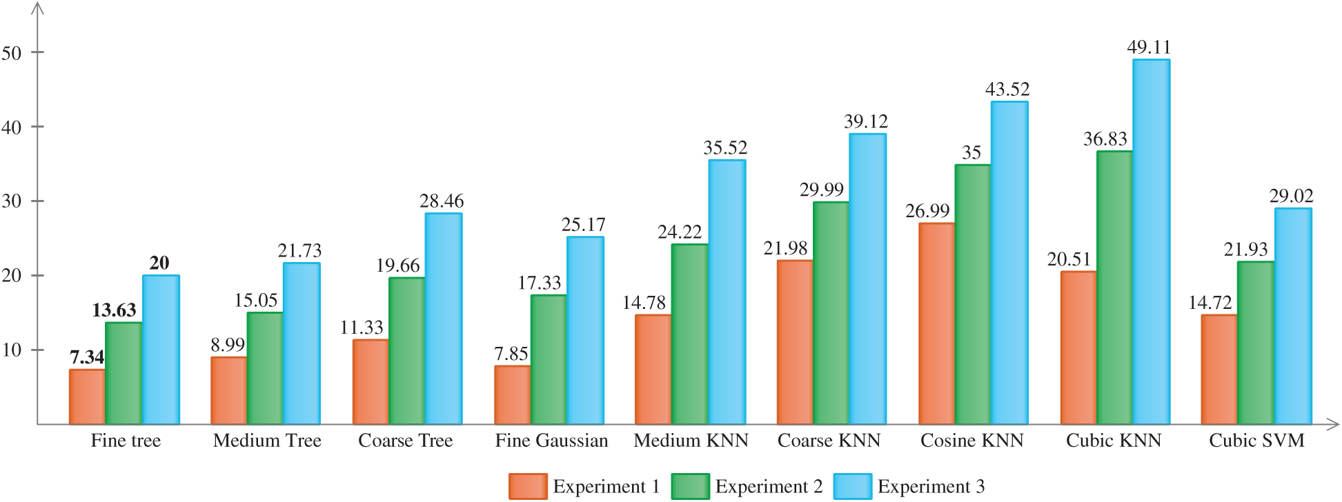
Figure 5: Computation time of testing data noted during the experimental process

This study focused on the identification of three common cotton leaf diseases using deep learning. A dataset was prepared for the three cotton diseases, and a pretrained deep model was reused using TL. Features were extracted from the different layers and serially combined into one vector for better feature representation instead of single-layer features. However, this process can affect the system's accuracy; therefore, we applied the GA for the best feature selection. The features selected through the GA maintained the accuracy and minimized the computational time during the testing process. Three experiments were conducted and a maximum accuracy of 98.8% was achieved for the approach considering 70/30 training/testing ratio. Overall, the performance of the proposed method was significant when using a prepared dataset. In the future, other cotton diseases will be considered for recognition. Moreover, the following improvements will be considered: (a) Collecting more images to increase the dataset; (b) utilizing the latest CNN model for recognition of cotton diseases; (c) selecting features based on meta-heuristic techniques, and (d) minimizing the recognition time for easy real-time processing.
Funding Statement: This work was supported by the Soonchunhyang University Research Fund.
Conflicts of Interest: The authors declare that they have no conflicts of interest to report regarding the present study.
1. M. Tauseef, F. Ihsan, W. Nazir and J. Farooq, “Weed flora and importance value index (IVI) of the weeds in cotton crop fields in the region of Khanewal, Pakistan,” Pakistan Journal of Weed Science Research, vol. 18, pp. 1–9, 2012. [Google Scholar]
2. A. Rehman, L. Jingdong, A. A. Chandio, I. Hussain, S. A. Wagan et al., “Economic perspectives of cotton crop in Pakistan: A time series analysis (1970–2015)(Part 1),” Journal of the Saudi Society of Agricultural Sciences, vol. 18, pp. 49–54, 2019. [Google Scholar]
3. M. S. Shabbir and N. Yaqoob, “The impact of technological advancement on total factor productivity of cotton: A comparative analysis between Pakistan and India,” Journal of Economic Structures, vol. 8, pp. 27, 2019. [Google Scholar]
4. T. Hussain, N. Akhtar and N. Butt, “Quality management: A case from Pakistan cotton yarn industry,” Journal of Quality and Technology Management, vol. 5, pp. 1–21, 2009. [Google Scholar]
5. R. Taqi, R. Talha, N. Ahmad, J. M. Uamr and U. Sami, “Diversity and abundance of insects in cotton crop land of punjab, Pakistan,” GSC Biological and Pharmaceutical Sciences, vol. 9, pp. 117–125, 2019. [Google Scholar]
6. M. S. Maqbool, H. ur Rehman, F. Bashir and R. Ahmad, “Investigating ‘Pakistan's revealed comparative advantage and competitiveness in cotton sector,” Review of Economics and Development Studies, vol. 5, pp. 125–134, 2019. [Google Scholar]
7. A. A. Khan and M. Khan, “Pakistan textile industry facing new challenges,” Research Journal of International Studies, vol. 14, pp. 21–29, 2010. [Google Scholar]
8. S. Mansoor, I. Amin, S. Iram, M. Hussain, Y. Zafar et al., “Breakdown of resistance in cotton to cotton leaf curl disease in Pakistan,” Plant Pathology, vol. 52, pp. 784–784, 2003. [Google Scholar]
9. Q. Xiao, W. Li, Y. Kai, P. Chen, J. Zhang et al., “Occurrence prediction of pests and diseases in cotton on the basis of weather factors by long short term memory network,” BMC Bioinformatics, vol. 20, pp. 688, 2019. [Google Scholar]
10. I. M. Nasir, A. Bibi, J. H. Shah, M. A. Khan, M. Sharif et al., “Deep learning-based classification of fruit diseases: An application for precision agriculture,” Computers, Materials & Continua, vol. 66, pp. 1949–1962, 2021. [Google Scholar]
11. N. Muhammad, Rubab, N. Bibi, O.-Y. Song, M. A. Khan et al., “Severity recognition of aloe vera diseases using AI in tensor flow domain,” Computers, Materials & Continua, vol. 66, pp. 2199–2216, 2021. [Google Scholar]
12. H. T. Rauf, B. A. Saleem, M. I. U. Lali and M. Sharif, “A citrus fruits and leaves dataset for detection and classification of citrus diseases through machine learning,” Data in Brief, vol. 26, pp. 104340, 2019. [Google Scholar]
13. T. Akram, M. Sharif and T. Saba, “Fruits diseases classification: Exploiting a hierarchical framework for deep features fusion and selection,” Multimedia Tools and Applications, vol. 79, pp. 25763–25783, 2020. [Google Scholar]
14. A. Adeel, M. A. Khan, T. Akram, A. Sharif, M. Yasmin et al., “Entropy-controlled deep features selection framework for grape leaf diseases recognition,” Expert Systems, vol. 2020, pp. 1–17, 2020. [Google Scholar]
15. K. Aurangzeb, F. Akmal, M. A. Khan, M. Sharif and M. Y. Javed, “Advanced machine learning algorithm based system for crops leaf diseases recognition,” in 6th Conf. on Data Science and Machine Learning Applications, Sakaka, SA, pp. 146–151, 2020. [Google Scholar]
16. M. A. Khan, T. Akram, M. Sharif, K. Javed, M. Raza et al., “An automated system for cucumber leaf diseased spot detection and classification using improved saliency method and deep features selection,” Multimedia Tools and Applications, vol. 8, pp. 1–30, 2020. [Google Scholar]
17. C. Webster and S. Ivanov, “Robotics, artificial intelligence, and the evolving nature of work,” in Digital Transformation in Business and Society, Cham: Springer, pp. 127–143, 2020. [Google Scholar]
18. A. Adeel, M. A. Khan, M. Sharif, F. Azam, J. H. Shah et al., “Diagnosis and recognition of grape leaf diseases: An automated system based on a novel saliency approach and canonical correlation analysis based multiple features fusion,” Sustainable Computing: Informatics and Systems, vol. 24, pp. 100349, 2019. [Google Scholar]
19. M. A. Khan, M. I. U. Lali, M. Sharif, K. Javed, K. Aurangzeb et al., “An optimized method for segmentation and classification of apple diseases based on strong correlation and genetic algorithm based feature selection,” IEEE Access, vol. 7, pp. 46261–46277, 2019. [Google Scholar]
20. F. de Oliveira Baldner, P. B. Costa, J. F. S. Gomes and F. R. Leta, “A review on computer vision applied to mechanical tests in search for better accuracy,” in Advances in Visualization and Optimization Techniques for Multidisciplinary Research, Cham: Springer, pp. 265–281, 2020. [Google Scholar]
21. A. Paul, S. Ghosh, A. K. Das, S. Goswami, S. D. Choudhury et al., “A review on agricultural advancement based on computer vision and machine learning,” in Emerging Technology in Modelling and Graphics, Cham: Springer, pp. 567–581, 2020. [Google Scholar]
22. R. Szeliski, “Computer vision: Algorithms and applications,” Instructor, vol. 201901, pp. 9–13, 2019. [Google Scholar]
23. S. Patel, A. Sarabakha, D. Kircali and E. Kayacan, “An intelligent hybrid artificial neural network-based approach for control of aerial robots,” Journal of Intelligent & Robotic Systems, vol. 7, pp. 1–12, 2019. [Google Scholar]
24. O. Caliskan, D. Kurt, N. Camas and M. S. Odabas, “Estimating chlorophyll concentration index in sugar beet leaves using an artificial neural network,” Polish Journal of Environmental Studies, vol. 29, pp. 1–7, 2020. [Google Scholar]
25. M. A. Khan, T. Akram, M. Sharif, M. Awais, K. Javed et al., “CCDF: Automatic system for segmentation and recognition of fruit crops diseases based on correlation coefficient and deep CNN features,” Computers and Electronics in Agriculture, vol. 155, pp. 220–236, 2018. [Google Scholar]
26. V. Singh and A. K. Misra, “Detection of plant leaf diseases using image segmentation and soft computing techniques,” Information Processing in Agriculture, vol. 4, pp. 41–49, 2017. [Google Scholar]
27. E. C. Too, L. Yujian, S. Njuki and L. Yingchun, “A comparative study of fine-tuning deep learning models for plant disease identification,” Computers and Electronics in Agriculture, vol. 161, pp. 272–279, 2019. [Google Scholar]
28. A. Sengupta, Y. Ye, R. Wang, C. Liu and K. Roy, “Going deeper in spiking neural networks: VGG and residual architectures,” Frontiers in Neuroscience, vol. 13, pp. 1–11, 2019. [Google Scholar]
29. G. Huang, Z. Liu, L. Van Der Maaten and K. Q. Weinberger, “Densely connected convolutional networks,” in Proc. of the IEEE Conf. on Computer Vision and Pattern Recognition, NY, USA, pp. 4700–4708, 2017. [Google Scholar]
30. Q. Wu, K. Zhang and J. Meng, “Identification of soybean leaf diseases via deep learning,” Journal of the Institution of Engineers, vol. 100, pp. 659–666, 2019. [Google Scholar]
31. R. Huang, L. Xi, X. Li, C. R. Liu, H. Qiu et al., “Residual life predictions for ball bearings based on self-organizing map and back propagation neural network methods,” Mechanical Systems and Signal Processing, vol. 21, pp. 193–207, 2007. [Google Scholar]
32. S. Zhang, X. Wu, Z. You and L. Zhang, “Leaf image based cucumber disease recognition using sparse representation classification,” Computers and Electronics in Agriculture, vol. 134, pp. 135–141, 2017. [Google Scholar]
33. Z. Iqbal, M. A. Khan, M. Sharif, J. H. Shah, M. H. ur Rehman et al., “An automated detection and classification of citrus plant diseases using image processing techniques: A review,” Computers and Electronics in Agriculture, vol. 153, pp. 12–32, 2018. [Google Scholar]
34. X. Glorot, A. Bordes and Y. Bengio, “Deep sparse rectifier neural networks,” in Proc. of the Fourteenth Int. Conf. on Artificial Intelligence and Statistics, NY, USA, pp. 315–323, 2011. [Google Scholar]
35. D. Macêdo, C. Zanchettin, A. L. Oliveira and T. Ludermir, “Enhancing batch normalized convolutional networks using displaced rectifier linear units: A systematic comparative study,” Expert Systems with Applications, vol. 124, pp. 271–281, 2019. [Google Scholar]
36. A. N. Gomez, I. Zhang, K. Swersky, Y. Gal and G. E. Hinton, “Learning sparse networks using targeted dropout,” arXiv preprint arXiv: 1905.13678, 2019. [Google Scholar]
37. S. J. Pan and Q. Yang, “A survey on transfer learning,” IEEE Transactions on Knowledge and Data Engineering, vol. 22, pp. 1345–1359, 2009. [Google Scholar]
38. H.-h. Zhao and H. Liu, “Multiple classifiers fusion and CNN feature extraction for handwritten digits recognition,” Granular Computing, vol. 8, pp. 1–8, 2019. [Google Scholar]
39. M. Rashid, M. A. Khan, M. Alhaisoni, S.-H. Wang, S. R. Naqvi et al., “A sustainable deep learning framework for object recognition using multi-layers deep features fusion and selection,” Sustainability, vol. 12, pp. 5037, 2020. [Google Scholar]
40. Z. u. Rehman, F. Ahmed, R. Damaševičius, S. R. Naqvi, W. Nisar et al., “Recognizing apple leaf diseases using a novel parallel real-time processing framework based on MASK RCNN and transfer learning: An application for smart agriculture,” IET Image Processing, vol. 1, pp. 1–23, 2021. [Google Scholar]
41. J. Kianat, M. Sharif, T. Akram, A. Rehman and T. Saba, “A joint framework of feature reduction and robust feature selection for cucumber leaf diseases recognition,” Optik, vol. 3, pp. 1–26, 2021. [Google Scholar]
42. F. Saeed, M. Mittal, L. M. Goyal and S. Roy, “Deep neural network features fusion and selection based on PLS regression with an application for crops diseases classification,” Applied Soft Computing, vol. 103, pp. 44–64, 2021. [Google Scholar]
43. M. B. Tahir, K. Javed, S. Kadry, Y.-D. Zhang, T. Akram et al., “Recognition of apple leaf diseases using deep learning and variances-controlled features reduction,” Microprocessors and Microsystems, vol. 1, pp. 104027–104050, 2021. [Google Scholar]
44. M. I. Sharif, M. Alhussein, K. Aurangzeb, and M. Raza, “A decision support system for multimodal brain tumor classification using deep learning,” Complex and Intelligent Systems, vol. 2, pp. 1–14, 2021. [Google Scholar]
45. K. Muhammad, M. Sharif, T. Akram and V. H. C. de Albuquerque, “Multi-class skin lesion detection and classification via teledermatology,” IEEE Journal of Biomedical and Health Informatics, vol. 1, pp. 1–9, 2021. [Google Scholar]
46. A. Majid, M. A. Khan, M. Yasmin, A. Rehman, A. Yousafzai et al., “Classification of stomach infections: A paradigm of convolutional neural network along with classical features fusion and selection,” Microscopy Research and Technique, vol. 83, pp. 562–576, 2020. [Google Scholar]
 | This work is licensed under a Creative Commons Attribution 4.0 International License, which permits unrestricted use, distribution, and reproduction in any medium, provided the original work is properly cited. |