DOI:10.32604/cmc.2021.015920
| Computers, Materials & Continua DOI:10.32604/cmc.2021.015920 | |
| Article |
Gastrointestinal Tract Infections Classification Using Deep Learning
1Department of Computer Science, COMSATS University Islamabad, Wah Campus, 47040, Pakistan
2Department of Computer Science, HITEC University Taxila, Taxila, 47080, Pakistan
3Department of Computer Science and Engineering, Soonchunhyang University, Asan, Korea
*Corresponding Author: Yunyoung Nam. Email: ynam@sch.ac.kr
Received: 14 December 2020; Accepted: 29 March 2021
Abstract: Automatic gastrointestinal (GI) tract disease recognition is an important application of biomedical image processing. Conventionally, microscopic analysis of pathological tissue is used to detect abnormal areas of the GI tract. The procedure is subjective and results in significant inter-/intra-observer variations in disease detection. Moreover, a huge frame rate in video endoscopy is an overhead for the pathological findings of gastroenterologists to observe every frame with a detailed examination. Consequently, there is a huge demand for a reliable computer-aided diagnostic system (CADx) for diagnosing GI tract diseases. In this work, a CADx was proposed for the diagnosis and classification of GI tract diseases. A novel framework is presented where preprocessing (LAB color space) is performed first; then local binary patterns (LBP) or texture and deep learning (inceptionNet, ResNet50, and VGG-16) features are fused serially to improve the prediction of the abnormalities in the GI tract. Additionally, principal component analysis (PCA), entropy, and minimum redundancy and maximum relevance (mRMR) feature selection methods were analyzed to acquire the optimized characteristics, and various classifiers were trained using the fused features. Open-source color image datasets (KVASIR, NERTHUS, and stomach ULCER) were used for performance evaluation. The study revealed that the subspace discriminant classifier provided an efficient result with 95.02% accuracy on the KVASIR dataset, which proved to be better than the existing state-of-the-art approaches.
Keywords: Convolutional neural network; feature fusion; gastrointestinal tract; handcrafted features; features selection
The medical industry is adopting advanced technology, through which it can improve healthy living. With the help of endoscopy and other techniques, medical doctors can visualize the human body’s internal tracts from the mouth to the intestines that were unapproachable in the past. Generally, the vast expertise of medical doctors is desired for problem recognition in the {gastrointestinal} (GI) tract [1]. Upper endoscopy and colonoscopy are the two main endoscopic methods. A tube is inserted through the mouth, throat, and stomach in the upper endoscopy method, and the small intestine is examined. During colonoscopy, the tube is inserted through the anus to examine the rectum and colon. The lower part of the GI tract consists of the bowel, which is influenced by several illnesses, such as cancer and incessant aggravation.
In the United States, 60–70 million people are affected by GI diseases every year [2]. Early examination and tests are carried out to detect colon disorders with the help of colonoscopy. The screening test procedure requires significant time for the medical specialist and high costs, which causes an unpleasant environment and dissatisfaction for the patients. Norway and the United States have performed tests that cost $450 and $1100 per case of GI complaint, respectively [3].
Several research methodologies improve the health care system by using technologies, such as artificial intelligence, multimedia data analyses, and distributed processing [4]. Several research societies have offered many proposals for automatic abnormality detection in the GI tract [5]. Different diagnostic imaging modalities are used for diagnosing human body abnormalities, such as CT scan, X-ray, and MRI. However, GI tract abnormalities are observed through colonoscopy and endoscopy (traditional and wireless) [6]. A challenge with endoscopy is that it is time consuming for gastroenterologists to go through each image and mark irregularities, making the procedure hectic and costly [7]. Similarly, colonoscopy faces miss rate challenges because doctors fail to find abnormalities.
Wireless capsule endoscopy consists of a CMOS camera that is to be swallowed by a patient. The capsule endoscopy camera transmits the captured images to a receiving digital storage unit for up to 7 h. After swallowing, the patient can perform normal activities as usual [8]. In contrast, the traditional wired video endoscopy in which the gastroenterologist can control the wire to observe the desired area in the GI tract, while in capsule endoscopy, captured frames are beyond the control of the gastroenterologist. Therefore, the fundamental aim of this study was to predict the variations from the norm in the GI tract through wired endoscopy. The major goal is to resolve the multi-class categorization issue in the GI tract by characterizing GI tract pictures into various categories. A computer-aided diagnostic system (CADx) assists medical experts in diagnosing and detecting abnormalities by providing an effective assistant for pathological findings. Therefore, the demand for medical image datasets is increasing worldwide for automatic disease detection, recognition, and assessment. Deep learning models are becoming vital players in spotting abnormalities in the GI tract.
The proposed method was explored in five steps. Preprocessing is the first step in which histogram equalization and color space transformation methods are employed for image enhancement. Visual information is learned in the second phase using handcrafted and deep learning methods. Accordingly, the local binary patterns (LBP) method is adopted to extract handcrafted features, while inceptionNet, ResNet50, and VGG-16 are utilized for acquiring deep features. Principal component analysis (PCA), entropy, and minimum redundancy and maximum relevance (mRMR) were analyzed in the third step, which improved the classification accuracy. In the fourth step, feature fusion is employed serially. The last and most important phase is classification, where several supervised classifiers are trained using integrated features. The proposed model is compared with several state-of-the-art methods. We observed that the proposed approach achieved improved results and performance.
The manuscript is styled as follows: Related works are presented in Section 2; Section 3 details the proposed approach; Section 4 highlights the outcomes of the tests performed; Section 5 summarizes the achievements.
Endoscopy is the key for the treatment and diagnosis of diseases in the GI tract. CADx systems have recently been introduced, in which existing endoscopy procedures involving operator variations are diminished and guided for accurate diagnoses of the disease [9]. The CADx system classifies diseases found in the GI tract using the training and testing feature sets. Generally, classification task results are based on methods, such as preprocessing, feature extraction, and feature selection. Additionally, preprocessing involves segmentation and image enhancement processes that help diagnose illness in the GI tract [10]. Feature extraction enriches system accuracy and endures system computation [7]. It is categorized into two methods: handcrafted and deep learning. Handcrafted features include shape (superpixel), texture (Gabor), and statistical, cellular, and color features. Meaningful handcrafted approaches help refine features to classify melanoma dermoscopy images [11]. Additionally, color features are valuable and return the location information of the disease, and shape features include a histogram of oriented gradient (HOG) [12], and segmentation-based fractal texture analyses (SFTA) are employed to acquire the features from the grayscale image to obtain information on the shape gradient and orientation. LBP features render the information of image patterns from color images [12,13]. In the past decades, extracting well-organized and optimized image features has been the primary goal of image classification tasks. Information from the images was extracted from different perspectives, such as handcrafted features using a color histogram [14], which calculates the color distribution of the images. Similarly, edges and texture information are collected by Gabor and LBP, whereas HOG can extract shape information that helps in disease detection. However, handcrafted features failed to detect the features of all aspects in the frames. Thus, the syndicate features of the deep convolutional neural network (CNN), and handcrafted features have been utilized.
Additionally, CNN models, such as AlexNet, ResNet50, inceptionNet, and VGG16 Net learn visualized features more precisely than handcrafted features. Therefore, the performance of CNN in the image recognition task is outstanding; however, various handcrafted features still play an important role in some domains. Handcrafted features provide image content from specific aspects, contrary to information for CNN in image classification tasks. The CNN learns features automatically, and thus it is difficult to understand the kind of features learned by the network. Using a CNN, it is difficult to control the composite features of a network. Therefore, some researchers have attempted to understand the interpretability and explainability of networks [15]. Therefore, in many studies, handcrafted and CNN features have been studied and implemented. These studies provide ideas of links between CNN and handcrafted features; therefore, it has now become a new research area in computer vision and image processing. Transfer learning techniques are introduced with different classification learning techniques without redesigning neural networks; moreover, classification performance is evaluated, and diseases are automatically detected [16]. In previous studies, feature fusion was introduced, where CNN and handcrafted features were fused, and in some domains, many handcrafted features played an important role; however, the obtained information did not describe all aspects of images, so, CNN features were introduced with handcrafted features [17]. Therefore, deep learning and texture features are integrated so that the performance of the model can be enhanced and domain information can be extracted from the frames of endoscopy, and multimedia content and machine learning techniques can be explored [18].
In the this study, a novel framework is presented that comprises five phases: preprocessing, feature extraction, feature selection, feature fusion, and classification methods. The LAB color space transformation and histogram equalization methods were used in the preprocessing phase to increase the accuracy of the model. The CNN learns features and handcrafted methods, and feature selection methods, such as PCA, entropy, and mRMR are analyzed using the selection of features alternatively. Additionally, the proposed study is confined to the feature fusion approach, where CNN and handcrafted features are fused, and later, train various classifiers. Fig. 1 shows the proposed model. The proposed model results were compared with existing state-of-the-art methods, which proved the effectiveness and robustness of the model. The steps of the proposed model are discussed in detail in the following section.
In this study, the transformation of the L*a*b* color space was performed, and the individual components of L*a*b* were extracted. The luminance of L* components was equalized by the histogram equalization method, and later, the L* components were merged with a*b* components that resulted in an enhanced L*a*b* frame. The complete KVASIR dataset, which consists of 4000 frames, was enhanced using this method. Preprocessing improves the overall performance of the model. The preprocessing process is illustrated in Fig. 2. The L*a*b* space evaluates colors better than the RGB color space and separates the luminosity and color. The L*a*b color space comprises three channels: luminosity L*, chromaticity a*, and b*, where L* represents different ranges of colors, such as black represents 0 level and 100 represents white levels. Similarly, a* and b* both have intensity values ranging from −128 to +127.
Moreover, L* components are used to adjust the contrast that closely matches the human perception of luminosity. Therefore, for transformation to the L*a*b* space, RGB channels are first converted to CIR channels and then to L*a*b* space channels. The L* transformation is expressed as follows:
where
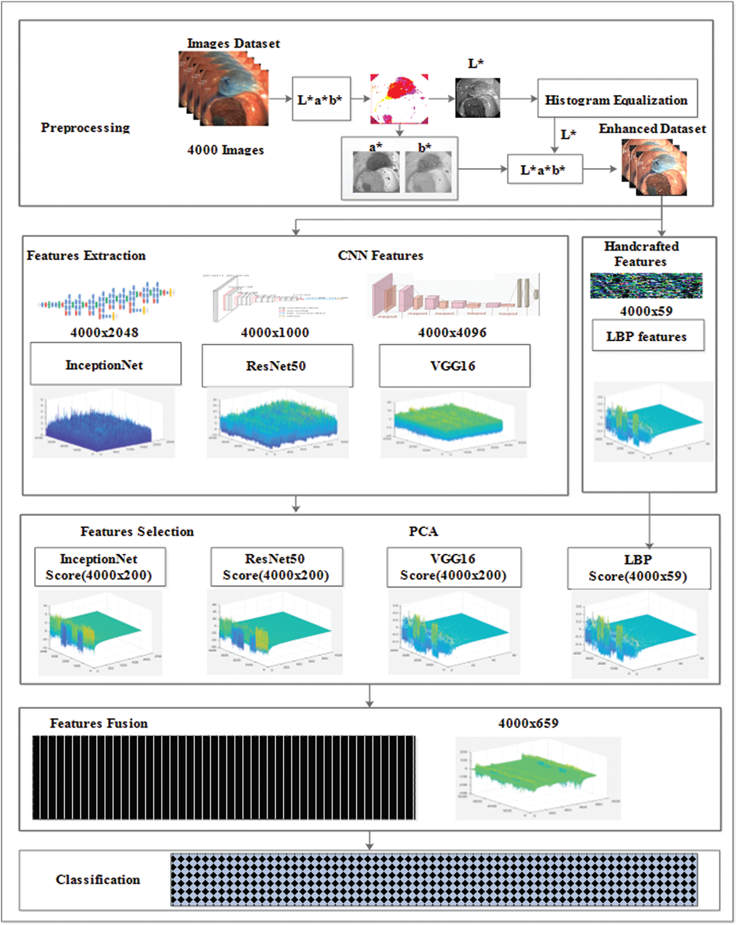
Figure 1: CNN and handcrafted features fusion model
Detailed information cannot be represented efficiently when the images are in raw form. Therefore, descriptors were used for feature extraction from which abnormalities were found in the images. There are several types of features in the image processing domain, such as the spatial and frequency domains. A special temporal domain is employed for feature acquisition through endoscopic images. The techniques of feature extraction and reduction have become essential in computer vision owing to applications, such as agriculture, robotics, surveillance, and medicine. The purpose of feature acquisition is to transform the input image data such that significant information can be extracted. Thus, the focus of feature extraction is to reduce the computation time and enhance the overall system performance. The two methods, handcrafted and CNN methods, are considered for feature acquisition.
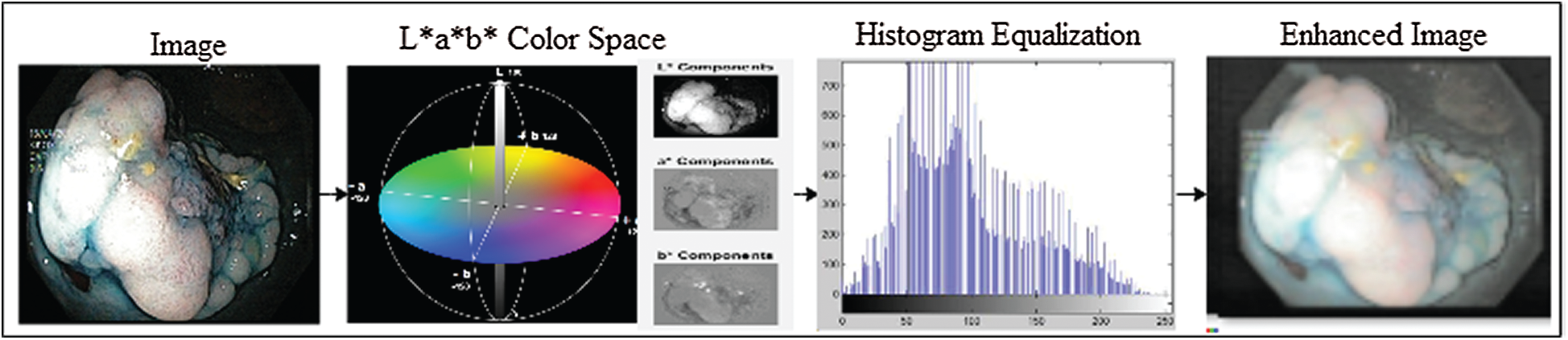
Figure 2: Image enhancement with L*a*b color space and histogram equalization methods
3.2.1 Handcrafted Features Extraction
Several methods are used for feature extraction; however, LBP features return the best performance with a combination of deep features. Hence, the LBP feature extraction method was employed in this study. The LBP operator represents texture information [19]. The LBP code represents the circular neighborhood of the pixel. Let
After LBP-based feature extraction, the histogram is constructed to represent an image and used as pattern recognition, known as features. Fig. 3 illustrates the visualization of the extracted LBP features.
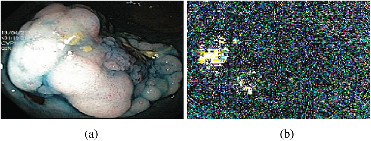
Figure 3: LBP features (a) Original image (b) Visual features
Generally, feature extraction techniques based on CNNs are used in several problems of image processing [20], such as face recognition and breast cancer mitosis detection [21,22]. In this study, various experiments were performed for feature extraction (visual information) using various deep learning models; however, the best results were achieved from the three transfer learning models, namely ResNet50 [23], InceptionNet [24], and VGG16 [25].
The architecture of the VGG16 model is a series network consisting of 41 layers. The network accepts a 224 × 224 size dimension as its input; the most repeated active layers in the network are the convolutional layers, rectified linear unit (ReLU), and max-pooling layers. It had a total of 16 convolutional layers, where 13 layers are convolutional, and three layers are fully connected. The first convolutional layer had a 3 × 3 filter size, and stride and padding were set to one. The features were acquired from the flattened layer, referred to as a fully connected (fc7) layer with an output size of 1 × 1 × 4096, weight size of 4096 × 4096, and bias of 4096 × 1. Finally, the network provides 4000 × 4096 features set over the complete dataset. Fig. 4 shows the architecture of VGG16, including visual features selected from the convolutional 4, convolutional 5_1, convolutional 5_2, and convolutional 5_3 layers.
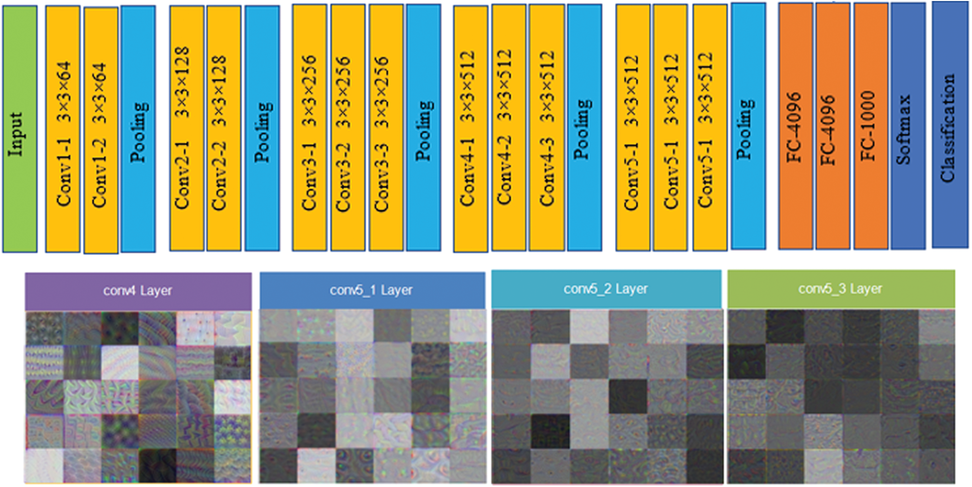
Figure 4: VGG16 architecture and visual features selected from convolutional layers (conv 4, conv 5_1, conv 5_2 and conv 5_3 layers)
The architecture of the ResNet50 model, referred to as a directed acyclic graph (DAG) network, consists of 177 layers. The architecture comprises five stages, where a convolutional layer and identity block are found in each stage. Additionally, there are three convolutional layers in a single convolutional block, and each identity block consists of three convolutional layers. The network accepts 224 × 224 size dimensions as its input; the most repeated active layers in the network are convolutional, batch normalization, ReLU, and max-pooling layers. The first convolutional layer contains a 7 × 7 size filter with a depth of 64, using padding 3. After the convolutional layer, the batch normalization layer was computed with 64 channels. The next layer is max pooling with stride 2, and padding 0. Convolutional and other processes are repeated by applying more layers to create a denser network, which can have a better impact on the accuracy, however the computational power also increases, which cannot be ignored. The features are acquired from the fully connected layer, which has an output size of 1 × 1 × 1000, weight size of 1000 × 2048, and bias of 1000 × 1; finally, the network provides 4000 × 1000 features over the complete dataset. Fig. 5 shows the architecture of VGG16 and visual features that are selected from layers, such as res2b_branch2a, res3c_branch2c, res4f_branch2b, and res5c_branch2a.
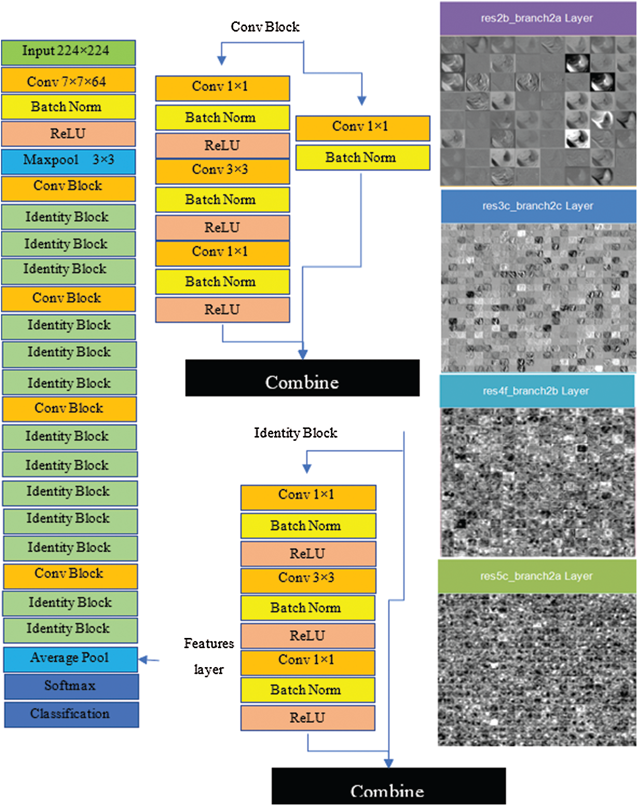
Figure 5: Resnet50 architecture and visual features selected from layers (res2b_branch2a, res3c_branch2c, res4f_branch2b and res5c_branch2a)
The architecture of the inceptionNet model is a convolution-based DAG network consisting of 316 layers. The network accepts 229 × 229 size dimensions as its input; the most repeated active layers in the network are the convolutional layers, batch normalization layers, average pooling, depth concatenation, ReLU, and max-pooling layers. The entire network branches are joined together at the depth concatenation point, where the network is also divided into four or three branches that represent a dense network. The features are acquired from the average pooling layer (avg_pool) in the network which has an output size of 1 × 1 × 20481, offset of 1 × 1 × 320, and a scale of 1 × 1 × 320; finally, the network provides 4000 × 2048 features over the entire dataset. Fig. 6 shows the visual features that were selected from convolutional layers, such as conv2d_1, conv2d_10, conv2d_52, and conv2d_94. Image recognition performance has been improved by deep CNN in recent years. InceptionNet is an example of a deep neural network; therefore, a very good performance is achieved using this architecture, while the computation cost is very low. The accuracy achieved is credible when the CNN is used in a composite fashion. The number of convolutional layers of VGG16 is greater than that of AlexNet, and this CNN retains three fully connected layers [26]. Adding the features of the VGG16 network with InceptionNet and ResNet50 features in the feature fusion matrix causes an improvement in the overall efficiency of the proposed model (see Fig. 7 for a detailed view of extracted features and their fusion after feature selection). In the same manner, in Fig. 7, the feature extraction method including a single frame is represented, whereas features of all 4000 frames are extracted from the KVASIR dataset. The size of the feature vector of the same image was different when using different CNN models, such as ResNet50 (1 × 1000), InceptionNet (1 × 2048), VGG16 (1 × 4096), and LBP (1 × 59). However, when the visual features of 4000 frames are extracted, the size of the feature set of every model becomes ResNet50 (4000 × 1000), InceptionNet (4000 × 2048), VGG16 (4000 × 4096), and LBP (4000 × 59). Subsequently, the best scores are computed by PCA, entropy, and mRMR methods using the extracted features, which are then fused in a serial fashion that is used by various classifiers for GI tract disease classification.
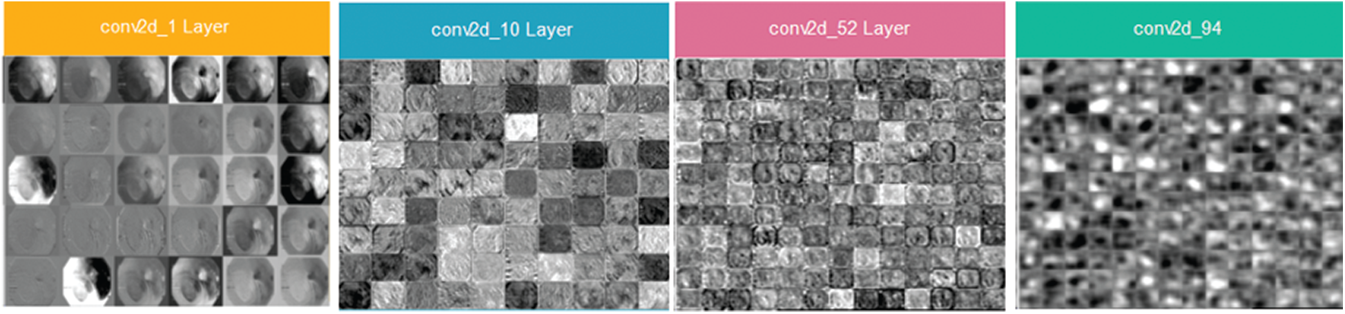
Figure 6: Inceptionv3 architecture and visual features selected from layers (conv2d_1, conv2d_10, conv2d_52 and conv2d_94)
Three feature selection approaches are analyzed for better feature selection in this study.
Feature selection methods, such as PCA, is used to reduce the size of the feature vectors. PCA is utilized for the transformation of the correlated variable into uncorrelated variables, also called clusters, and to calculate the optimized distance between each cluster to draw principal components between them. Moreover, PCA computes the learned features, such as handcrafted and deep CNN extracted features. In addition, the dataset contains information on the common structure of latent content extracted by PCA. Generally, when the dataset size is very large, PCA is considered a popular technique in multivariate scenarios [27]. The first and second principal components,
The first component shows the greatest variance among components in the sample space, and
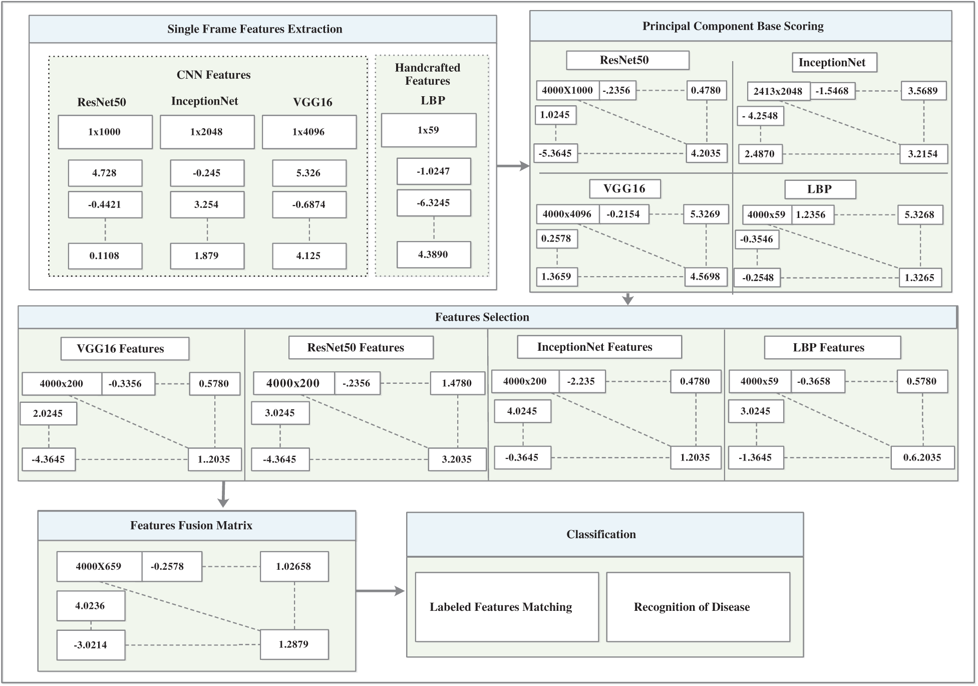
Figure 7: CNN and handcrafted features extraction, selection and fusion model
All transformations are performed mostly in matrix multiplication, which makes computation fast, and P is the overall PCA transformation of the variables, where A is the eigenvector and diagonal elements are called eigenvalues, which are explained by each principal component [28].
Entropy is an optimal feature searching algorithm that resolves the problem of the selected initial population. It reduces the features based on the highest entropy and computes them repeatedly up to the final optimal features. The entropy finds the root node and computes all entities [29].
Then the entropy of
3.3.3 Minimal-Redundancy-Maximal-Relevance (mRMR)
The heuristic techniques for removing redundant features in the dataset are known as mRMR [30]. The specific and optimal characteristics were obtained using this method without compromising the classification accuracy. High-dimensional data increase the error rate of the learning algorithms and cause overfitting of the model. However, the best features are selected based on the principal component, entropy, and mRMR. Moreover, the dimensions of the learned features set were characterized as ResNet50 (4000 × 1000), InceptionNet (4000 × 2048), VGG16 (4000 × 4096), and LBP (4000 × 59), which are illustrated as ResNet50 (4000 × 200), InceptionNet (4000 × 200), VGG16 (4000 × 200), and LBP (4000 × 59), which provide the best performance of the model.
In the proposed study, various methods of transfer learning are employed, such as ResNet50, InceptionNet, and VGG16 for feature learning. Several texture feature methods are utilized, such as LBP, to obtain texture information. However, the best performing deep learning and handcrafted feature models were selected and represented in this study. The novel approach of feature fusion is implemented in which the deep model learned features and texture information of the LBP model were fused serially. The individual feature sets of each method are represented as:
where r is the features set of LBP having dimensions 4000 × 59.
where s is the features set of ResNet having dimensions 4000 × 200.
where t is the features set of VGG having dimensions 4000 × 200.
where u is the features set of an inceptionNet having dimensions 4000 × 200. The individual feature sets are fused with serial concatenation as
In the classification method, anomalies are identified and classified by a classifier that takes a set of fused features at its input and predicts the class label after feature computation. The accuracy depends on several factors, such as the weight initialization activation function and the selection of deep layers. Moreover, image preprocessing, learned features, and feature fusion methods also play an important role in enhancing the model accuracy. However, several classifiers were trained to predict abnormalities in the frames of the GI tract. In this manner, many classifiers have been investigated, including linear discriminant, linear support vector machine (SVM), cubic SVM, coarse Gaussian SVM, cosine KNN, and subspace discriminant. Consequently, subspace discriminant analysis achieved a high score in accuracy when compared with the other classifiers.
4 Experimental Setup and Results
The performance of the CADx was evaluated in the this study, where the anomalies of the GI tract were automatically detected and classified using endoscopic frames. Moreover, experiments are performed using KVASIR as the main dataset, which consists of eight different classes, such as three normal and five disease classes of endoscopic frames. Similarly, the model was also evaluated with two other datasets, ULCER and NERTHUS, as state-of-the-art system evaluations. The evaluation metrics addressed in the prevailing publications are also compared. The proposed model’s results are reported in tabular form, where features, such as LBP, ResNet50, inceptionNet, and VGG16 deep CNN models are used for feature learning. The learned features are then serially fused. Similarly, several tests were carried out, and three of them were chosen based on high performance. Additionally, the selected models provided the best results in this study. The system used for all the evaluations was an Intel Core i5-4200U CPU running at 1.60 GHz and 8 GB RAM.
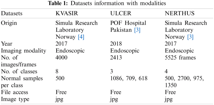
Three datasets, KVASIR [32], NERTHUS [33], and ULCER [13] were considered in this study. Annotated KVASIR consists of 4000 images with eight categories, each class containing 500 images. Of the eight classes, a single frame of each class is illustrated in Fig. 8. The major issues faced by qualified staff are high dimensionality and great similarities between certain disorders. ULCER datasets consist of 2413 images with three classes namely, bleeding, healthy, and ulcer. The bleeding class contains 1086 images, the healthy class contains 709 images, and the ulcer class contains 618 images. This dataset was obtained by colonoscopy.
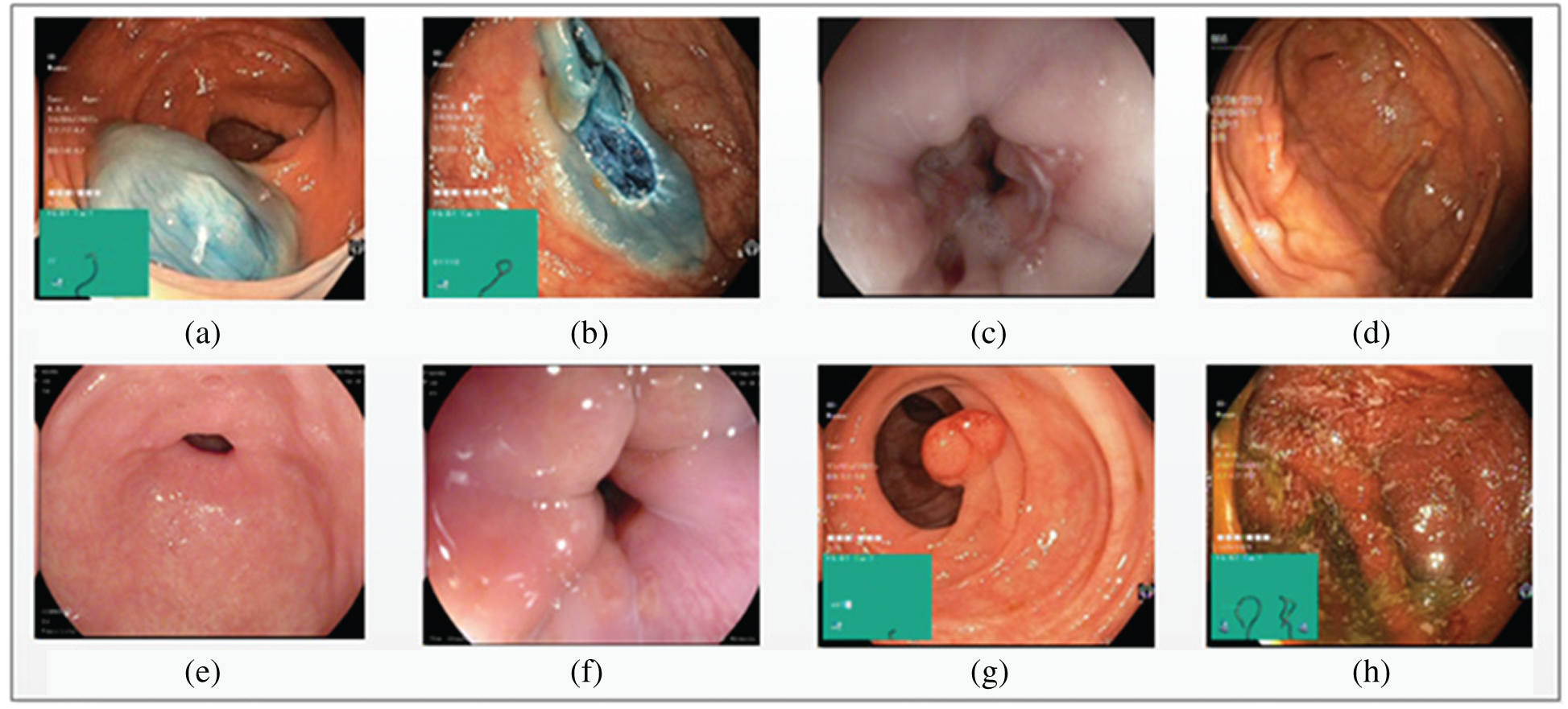
Figure 8: Eight types of classes taken from KVASIR dataset (a) Dyed-Lifted-Polyp (b) Dyed-Resection-Margins (c) Esophagitis (d) Normal-Cecum (e) Normal-Pylorus (f) Normal-z-Line (g) Polyps (h) Ulcerative-Colitis
It is an open-source dataset that shows different degrees of bowel cleansing in the GI tract. The NERTHUS dataset comprises a total of 5525 bowel frames from 21 videos [33]. Tab. 1 lists the details of each of the datasets mentioned above.
4.2 Overview of Conducted Experiments on KVASIR Dataset
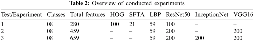
Various experiments were performed to improve the performance of the proposed model. Of the several tests, only three that show the best results are presented. A summary of the three tests performed is presented in Tab. 2. Each test contained eight classes and 4000 images of the GI tract, test1 contained collectively 280 features, such as HOG (100), SFTA (21), LBP (59), and AlexNet (100) features, test2 contained collectively 459 features, such as LBP (59), ResNet50 (200), and VGG16 (200) features, and test3 contained collectively 659 features, such as LBP (59), ResNet50 (200), InceptionNet (200), and VGG16 (200) features. Performance measurement parameters were calculated for each test. Test3 reported the best results compared to previous studies.
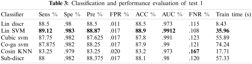
4.2.1 Test 1(HOG = 100, SFTA = 21, LBP = 59, RESNET = 100 KVASIR DATASET)
In experiment 1, one class out of eight classes contained 500 images; therefore, 4000 images were used collectively. A 10-fold cross-validation was utilized to evaluate all outcomes. From several classifiers, only six classifiers were trained, as shown in Tab. 3. Linear SVM performed well when compared to other classification methods, with an accuracy of 88.9, by consuming a training time of 35.96 s. The performance evaluation of test1 is presented in Tab. 3.
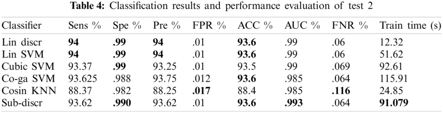
4.2.2 Test 2(LBP = 59, RESNET = 200, VGG16 = 200 KVASIR DATASET)
In this experiment, 10-fold cross-validation was used to assess all the results. The subspace discriminant performance was better than other prediction techniques, with an accuracy of 93.62. and a training time of 91.079 s. The graphical comparisons of classification methods in terms of precision, sensitivity, accuracy, and training time are shown in Tab. 4.
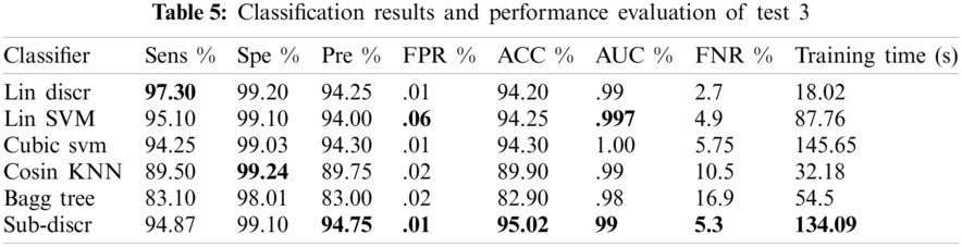
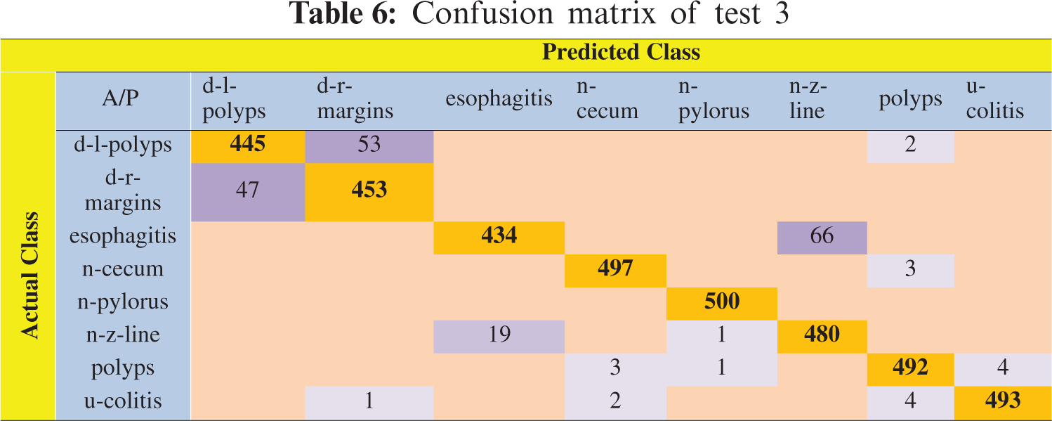
4.2.3 Test 3(LBP = 59, RESNET = 200, INCEPTIONNET = 200, VGG16 = 200 KVASIR DATASET)
In this experiment, 5-fold cross-validation was used to evaluate all results. A total of six classification methods were used. The subspace discriminant classifier's performance was the best in comparison to other prediction methods, with an accuracy of 95.02, and a training time of 134.09 s; this was found to outperform the methods prevalent in the literature. Graphical comparisons of classification methods in terms of precision, sensitivity, accuracy, and training time for test3 are presented in Tab. 5. The confusion matrix in Tab. 6 shows the satisfactory true positive values per class for test3.
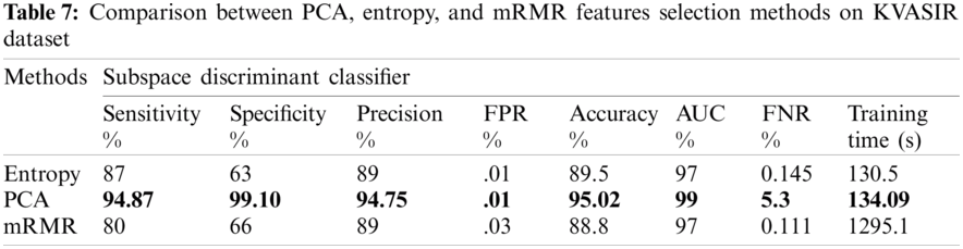
4.3 Analyzing Feature Selection Methods
Three feature selection approaches, PCA, mRMR, and entropy-based, were employed to check for optimal features. A performance comparison of these results is shown in Tab. 7.
The comparison highlights that the evaluation of the PCA method was better than that of the other feature selection methods. The maximum achieved accuracy was 95.02% using PCA, with a training time of 134.09 s, which shows that the proposed approach is better than the previous approaches. Based on the best results, we selected the configuration of test3, including the PCA feature selection method. This configuration is considered with other state-of-the-art configurations for comparison.
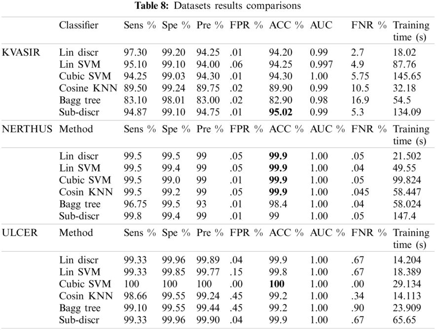
4.4 Results Comparisons Between KVASIR, NERTHUS and ULCER Datasets
The model performance was checked with the configurations mentioned in test3 on the other two datasets (NERTHUS and ULCER). The model also performed well, as shown in Tab. 8. A comparison of the six classifiers is presented in Tab. 8. Classifiers, such as linear discriminators, linear support vector machines, cubic SVMs, cosine KNNs, bagged trees, and subspace discriminators were used for classification. KVASIR was the most challenging dataset, with an accuracy of 95.02% on the Sub-Discr classifier. The best accuracy on the NERTHUS dataset was 99.9% for the four classifiers, as shown in Tab. 8. Cubic SVM showed the best results with an accuracy of 100% on the ULCER dataset. The subspace discriminator classifier showed stability and satisfactory accuracy on all datasets.
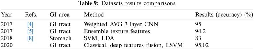
4.5 Comparisons with Existing Approaches
Tab. 9 depicts the comparison of the proposed method with the existing approaches. The proposed system showed better results than the other methods.
Automatic disease detection and classification using endoscopic frames of the GI tract were addressed in the proposed study. The handcrafted features (LBP) and deep learning features (VGG16, inceptionNet, ResNet50) were extracted, and their subsets were selected using PCA, entropy, and mRMR feature selection methods. The subsets were then fused using the serial feature fusion method. Three datasets were used for the performance evaluation. High accuracies, such as 95.02%, 99.9%, and 100% on the KVASIR, NERTHUS, and ulcer datasets, respectively, were achieved. The most stable classifier was the Sub-Discr classifier with a satisfactory overall accuracy. Our experiments show that techniques such as preprocessing and feature fusion are efficient techniques that boost the overall performance of the model. Although using this method, we achieved a fairly high accuracy compared with existing approaches, there is still scope for further improvement which must be addressed in future research. Using other preprocessing techniques and deep learning models for feature extraction can improve model performance.
Funding Statement: This research was supported by Korea Institute for Advancement of Technology (KIAT) grant funded by the Korea Government (MOTIE) (P0012724, The Competency Development Program for Industry Specialist) and the Soonchunhyang University Research Fund.
Conflicts of Interest: The authors declare that they have no conflicts of interest to report regarding the present study.
1. A. Liaqat, M. A. Khan, M. Sharif, M. Mittal, T. Saba et al., “Gastric tract infections detection and classification from wireless capsule endoscopy using computer vision techniques: A review,” Current Medical Imaging, vol. 2, pp. 1–33, 2020. [Google Scholar]
2. N. Clearinghouse, Digestive Diseases Statistics for the United States. Bethesda, MD: National Institutes of Health, 2013. [Google Scholar]
3. M. Riegler, K. Pogorelov, P. Halvorsen, T. de Lange, C. Griwodz et al., “EIR—efficient computer aided diagnosis framework for gastrointestinal endoscopies,” in 2016 14th Int. Workshop on Content-Based Multimedia Indexing, Bucharest, Romania, pp. 1–6, 2016. [Google Scholar]
4. M. A. Khan, M. S. Sarfraz, M. Alhaisoni, A. A. Albesher, S. Wang et al., “StomachNet: Optimal deep learning features fusion for stomach abnormalities classification,” IEEE Access, vol. 8, pp. 197969–197981, 2020. [Google Scholar]
5. J. Naz, M. Sharif, M. Yasmin, M. Raza and M. A. Khan, “Detection and classification of gastrointestinal diseases using machine learning,” Current Medical Imaging, vol. 2, no. 1, pp. 1–21, 2020. [Google Scholar]
6. M. A. Khan, S. Kadry, M. Alhaisoni, Y. Nam, Y. Zhang et al., “Computer-aided gastrointestinal diseases analysis from wireless capsule endoscopy: A framework of best features selection,” IEEE Access, vol. 8, pp. 132850–132859, 2020. [Google Scholar]
7. A. Majid, M. A. Khan, M. Yasmin, A. Rehman, A. Yousafzai et al., “Classification of stomach infections: A paradigm of convolutional neural network along with classical features fusion and selection,” Microscopy Research and Technique, vol. 83, no. 2, pp. 562–576, 2020. [Google Scholar]
8. M. Appleyard, Z. Fireman, A. Glukhovsky, H. Jacob, R. Shreiver et al., “A randomized trial comparing wireless capsule endoscopy with push enteroscopy for the detection of small-bowel lesions,” Gastroenterology, vol. 119, no. 6, pp. 1431–1438, 2000. [Google Scholar]
9. T. de Lange, P. Halvorsen and M. Riegler, “Methodology to develop machine learning algorithms to improve performance in gastrointestinal endoscopy,” World Journal Gastroenterol, vol. 24, no. 45, pp. 5057–5062, 2018. [Google Scholar]
10. A. A. Kalinin, V. I. Iglovikov, A. Rakhlin and A. A. Shvets, “Medical image segmentation using deep neural networks with pre-trained encoders,” in Deep Learning Applications, Cham: Springer, pp. 39–52, 2020. [Google Scholar]
11. J. Hagerty, J. Stanley, H. Almubarak, N. Lama, R. Kasmi et al., “Deep learning and handcrafted method fusion: Higher diagnostic accuracy for melanoma dermoscopy images,” IEEE Journal of Biomedical and Health Informatics, vol. 23, no. 4, pp. 1385–1391, 2019. [Google Scholar]
12. K. Pogorelov, M. Riegler, P. Halvorsen, C. Griwodz, T. de Lange et al., “A comparison of deep learning with global features for gastrointestinal disease detection,” MediaEval, 2017. [Google Scholar]
13. A. Liaqat, M. A. Khan, J. H. Shah, M. Sharif, M. Yasmin et al., “Automated ulcer and bleeding classification from WCE images using multiple features fusion and selection,” Journal of Mechanics in Medicine and Biology, vol. 18, no. 4, pp. 1850038, 2018. [Google Scholar]
14. X. Xing, X. Jia and M.-H. Meng, “Bleeding detection in wireless capsule endoscopy image video using superpixel-color histogram and a subspace KNN classifier,” in 2018 40th Annual Int. Conf. of the IEEE Engineering in Medicine and Biology Society, Honolulu, HI, USA, pp. 1–4, 2018. [Google Scholar]
15. D. Bau, B. Zhou, A. Khosla, A. Oliva and A. Torralba, “Network dissection: Quantifying interpretability of deep visual representations,” in Proc. of the IEEE Conf. on Computer Vision and Pattern Recognition, Honolulu, Hawaii, pp. 6541–6549, 2017. [Google Scholar]
16. O. Ostroukhova, K. Pogorelov, M. Riegler, D.-T. Dang-Nguyen and P. Halvorsen, “Transfer learning with prioritized classification and training dataset equalization for medical objects detection,” MediaEval, 2018. [Google Scholar]
17. Z. Tianyu, M. Zhenjiang and Z. Jianhu, “Combining CNN with hand-crafted features for image classification,” in 2018 14th IEEE Int. Conf. on Signal Processing, Beijing, China, pp. 554–557, 2018. [Google Scholar]
18. S. Nadeem, M. A. Tahir, S. S. A. Naqvi and M. Zaid, “Ensemble of texture and deep learning features for finding abnormalities in the gastro-intestinal tract,” in Int. Conf. on Computational Collective Intelligence, Cham: Springer, vol. 11056, pp. 469–478, 2018. [Google Scholar]
19. T. Tuncer, S. Dogan and F. Ertam, “A novel neural network based image descriptor for texture classification,” Physica A: Statistical Mechanics and Its Applications, vol. 526, pp. 120955, 2019. [Google Scholar]
20. X. Lin, Y. Rivenson, N. T. Yardimci, M. Veli, Y. Luo et al., “All-optical machine learning using diffractive deep neural networks,” Science, vol. 361, no. 6406, pp. 1004–1008, 2018. [Google Scholar]
21. D. C. Cireşan, A. Giusti, L. M. Gambardella and J. Schmidhuber, “Mitosis detection in breast cancer histology images with deep neural networks,” in Int. Conf. on Medical Image Computing and Computer-assisted Intervention, Berlin, Heidelberg, pp. 411–418, 2013. [Google Scholar]
22. S. Sornapudi, R. J. Stanley, W. V. Stoecker, H. Almubarak, R. Long et al., “Deep learning nuclei detection in digitized histology images by superpixels,” Journal of Pathology Informatics, vol. 9, no. 1, pp. 1–9, 2018. [Google Scholar]
23. S. Targ, D. Almeida and K. Lyman, “Resnet in resnet: Generalizing residual architectures,” arXiv preprint arXiv:1603.08029, 2016. [Google Scholar]
24. X. Wang, Y. Lu, Y. Wang and W.-B. Chen, “Diabetic retinopathy stage classification using convolutional neural networks,” in 2018 IEEE Int. Conf. on Information Reuse and Integration, Salt Lake City, UT, USA, pp. 465–471, 2018. [Google Scholar]
25. E. Rezende, G. Ruppert, T. Carvalho, A. Theophilo, F. Ramos et al., “Malicious software classification using VGG16 deep neural network’s bottleneck features,” in Information Technology-New Generations, Cham: Springer, pp. 51–59, 2018. [Google Scholar]
26. S. Han, J. Pool, J. Tran and W. Dally, “Learning both weights and connections for efficient neural network,” Advances in Neural Information Processing Systems, vol. 28, pp. 1135–1143, 2015. [Google Scholar]
27. Y. Aït-Sahalia and D. Xiu, “Principal component analysis of high-frequency data,” Journal of the American Statistical Association, vol. 114, no. 525, pp. 287–303, 2019. [Google Scholar]
28. S. M. Holland, Principal Components Analysis (PCA). Athens, GA: Department of Geology, University of Georgia, pp. 30602–32501, 2008. [Google Scholar]
29. M. A. Khan, M. Sharif, M. Y. Javed, T. Akram, M. Yasmin et al., “License number plate recognition system using entropy-based features selection approach with SVM,” IET Image Processing, vol. 12, no. 3, pp. 200–209, 2017. [Google Scholar]
30. C. Xu, S. Zhao and F. Liu, “Distributed plant-wide process monitoring based on PCA with minimal redundancy maximal relevance,” Chemometrics and Intelligent Laboratory Systems, vol. 169, pp. 53–63, 2017. [Google Scholar]
31. M. A. Khan, T. Akram, M. Sharif, M. Y. Javed, N. Muhammad et al., “An implementation of optimized framework for action classification using multilayers neural network on selected fused features,” Pattern Analysis and Applications, vol. 22, no. 4, pp. 1377–1397, 2019. [Google Scholar]
32. K. Pogorelov, K. R. Randel, C. Griwodz, S. L. Eskeland, T. de Lange et al., “Kvasir: A multi-class image dataset for computer aided gastrointestinal disease detection,” in Proc. of the 8th ACM on Multimedia Systems Conf., Taipei, Taiwan, pp. 164–169, 2017. [Google Scholar]
33. K. Pogorelov, K. R. Randel, T. de Lange, S. L. Eskeland, C. Griwodz et al., “Nerthus: A bowel preparation quality video dataset,” in Proc. of the 8th ACM on Multimedia Systems Conf., Taipei, Taiwan, pp. 170–174, 2017. [Google Scholar]
34. K. Pogorelov, P. T. Schmidt, M. Riegler, P. Halvorsen, K. R. Randel et al., “Kvasir,” in Proc. of the 8th ACM on Multimedia Systems Conf., Taipei, Taiwan, pp. 164–169, 2017. [Google Scholar]
35. S. S. A. Naqvi, S. Nadeem, M. Zaid and M. A. Tahir, “Ensemble of texture features for finding abnormalities in the gastro-intestinal tract,” in MediaEval, 2017. [Google Scholar]
 | This work is licensed under a Creative Commons Attribution 4.0 International License, which permits unrestricted use, distribution, and reproduction in any medium, provided the original work is properly cited. |