Computers, Materials & Continua DOI:10.32604/cmc.2021.019409
Article

A Multi-Category Brain Tumor Classification Method Bases on Improved ResNet50

Linguo Li1,2, Shujing Li1,* and Jian Su3

1Fuyang Normal University, Fuyang, 236041, China
2Nanjing University of Posts and Telecommunications, Nanjing, 210003, China
3University of Michigan, Ann Arbor, MI, 48109, USA
*Corresponding Author: Shujing Li. Email: lsjing1981@163.com
Received: 11 April 2021; Accepted: 12 May 2021

Abstract: Brain tumor is one of the most common tumors with high mortality. Early detection is of great significance for the treatment and rehabilitation of patients. The single channel convolution layer and pool layer of traditional convolutional neural network (CNN) structure can only accept limited local context information. And most of the current methods only focus on the classification of benign and malignant brain tumors, multi classification of brain tumors is not common. In response to these shortcomings, considering that convolution kernels of different sizes can extract more comprehensive features, we put forward the multi-size convolutional kernel module. And considering that the combination of average-pooling with max-pooling can realize the complementary of the high-dimensional information extracted by the two structures, we proposed the dual-channel pooling layer. Combining the two structures with ResNet50, we proposed an improved ResNet50 CNN for the applications in multi-category brain tumor classification. We used data enhancement before training to avoid model over fitting and used five-fold cross-validation in experiments. Finally, the experimental results show that the network proposed in this paper can effectively classify healthy brain, meningioma, diffuse astrocytoma, anaplastic oligodendroglioma and glioblastoma.

Keywords: Brain tumor; convolutional neural network; multi-size convolutional kernel module; dual-channel pooling layer; ResNet50

1  Introduction

Brain tumors are one of the most deadly cancers. Early detection plays an important role in the treatment and rehabilitation of patients. However, manual brain tumor diagnosis by physicians is a less accurate and time-consuming procedure [1]. Therefore, it is necessary to establish an intelligent and effective brain tumor classification system, which can help doctors analyze medical images and support specialists in making diagnoses at the early stage of tumor growth.

Medical image analysis has become a recent research hotspot. Machine learning and deep learning approaches in particular play core roles in computer-assisted brain image analysis, segmentation, registration, and tumor tissue classification [2–5]. At present, CNN is considered to be the most successful image processing method [6]. Instead of matrix multiplication, convolution operators are used in most layers of these networks. This contributes to the superiority of convolutional networks in solving problems with high computational costs. Another advantage of this method compared to shallow machine learning methods, is automatic feature extraction. Because of these advantages, CNN has also been widely used in the processing of medical images, such as grade classification [7], segmentation [8,9] and skull stripping of brain tumor images [10]. Establishing CAD [11] or multi-level brain tumor grading systems, supporting radiologist visualization [12] and identifying tumor types [13–15] using the deep neural network help radiologists make decisions on early diagnosis and future treatment.

2  Related Work

The detection of brain tumors has received extensive research attention, and various detection methods have been proposed in several years. Abd-Ellah [16] proposed a two-phase multi-model automatic brain tumor diagnosis system from magnetic resonance images using CNNs, in which the classification stage model consists of three parts, namely preprocessing, CNN feature extraction and error correction output code support vector machine (ECOC-SVM). The highest average accuracy of the model for benign and malignant brain tumor classification is 99.55%. Abdolmaleki et al. [17] developed a three-layer back-propagation neural network that distinguished between malignant and benign tumors using 13 different features. The magnetic resonance imaging (MRI) data they used for the experiment came from 165 patients, and the classification accuracy for benign and malignant tumors reached 91% and 94% respectively. These studies only focus on the binary classification of brain tumors, but only the benign and malignant classification is not enough for radiologists to decide on the treatment plan for the patients.

Sajjad [18] proposed a brain tumor classification method based on CNN. Firstly, the deep learning algorithm is used to segment the tumor region in MRI image, then the enhanced data set is used to fine tune the CNN model. The average accuracy of the model for four tumor classifications (Grade I-Grade IV) in radiopedia dataset is 87.38%. In 2020, Ghassemi [19] proposed a new deep learning method for MRI image classification of brain tumors. Firstly, a deep neural network is pre-trained on different data sets as a discriminator for generating confrontation network (GAN) to extract the robust features of MRI image and learn the structure of MRI image in its convolution layer, and then the softmax layer is used to replace the full connection layer of the network. The average classification accuracy of this method for meningioma, glioma and pituitary tumor is 93.01%. The above methods all use deep neural network [18,19], but with the increase of depth, the problem of gradient vanishing and over fitting will appear in the network.

3  Proposed Method

To solve the problem of gradient vanishing or gradient explosion when simply deepening the network, He proposed a deep convolutional residual network in 2015—-ResNet50 [20]. The ResNet50 network is built by residual modules. This type of modules not only makes the network free of degradation problems, but also reduces the error rate, and keeps the computational complexity at a very low level. Zhu [21] used the pre-trained ResNet50 to determine the invasion depth of gastric cancer. ResNet50 could be understood as a 5-stage one in total. After the first stage, the image was transformed into a tensor of 112 × 112 × 64. Then residual modules were introduced between Stage 2 and Stage 5 to overcome the problem of gradient disappearance and explosion. After five stages, the input was converted to a tensor of 7 × 7 × 2048, and the dimension increased from 3 to 2048, indicating that information extracted was more than the original RGB pixels.

Finally, according to the extracted 2048 features, the tensor was flattened into to a 4096-dimensional vector and then sent to softmax for classification. Taking the tumor classification in this paper as an example, let the final classification number K be five, and give a training set{(x1,y1), (x2,y2),…,(xm,ym)}, whereyi∈{1,2…k}. Now, given an input test data x, softmax estimates the probability of each class by calculating the corresponding probability value p(y=j|x) for each class, and finally outputs a k-dimensional normalized vector:

hθ(xi)=[p(y=1|xi;θ)p(y=2|xi;θ)…p(y=k|xi;θ)]=1∑kjeθTjxi[eθT1xieθT2xi…eθTkxi](1)

where θ1,…,θk∈ℜn+1 is the model parameters, the final output vector of each element corresponding to the corresponding probability estimate of a tumor category, the sum of all elements is 1.

Due to the excellent structure of the residual network, ResNet50 was selected for the experiment and two improvements were made to it. The improved network structure is shown in Fig. 1.

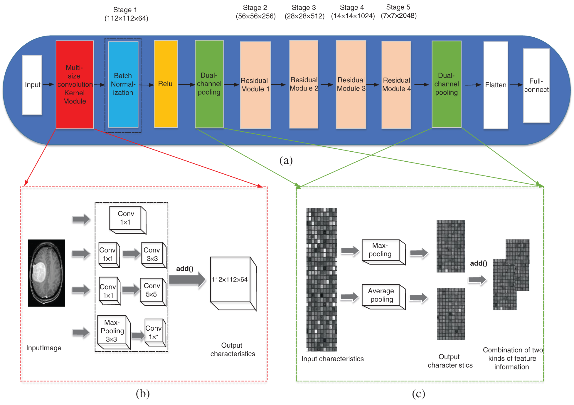
Figure 1: The improved network structure. (a) Improved ResNet50 network structure, (b) Multi-size convolutional kernel module, (c) Dual-channel pooling layer

In the literature [22], an inception v1 module was proposed, which improved in network width. Inspired by the inception v1 module, this paper proposed a multi-size convolutional kernel module similar to inception v1, as is shown in Fig. 1b, to replace the 7 × 7 convolution layer of Stage 1 in the ResNet50 network. This is because convolution kernels of different sizes can extract features of different sizes, and can also take the details of the surrounding area of each pixel and the features of the larger background (for example, whether it is close to the skull) into account [23]. This makes the features input into the residual module are more comprehensive and helps to improve the classification accuracy of the network. The difference between multi-size convolutional kernel module and inception v1 is that it used add( ) function instead of the concat( ) function to connect the various branches.

Suppose that the input characteristic dimension of the multi-size convolutional kernel module is W×H, the number of channels in each branch of the module is C, and the output characteristic dimension after concat( ) is Oc, and the output characteristic dimension after using add( ) is Oa:

Oc=W×H×4C(2)

Oa=W×H×C(3)

The concat( ) function only adds the dimension describing the features of the image itself when used for the combination of channels, and the feature information under each dimension is not added. Although the add() function does not add the dimensions describing the features of the image itself, the amount of information under each dimension increases, which is obviously beneficial to the classification of the final images.

In ResNet50 network, there is only a pooling layer after Stage 1 and Stage 5, which are max-pooling and average-pooling respectively. The pooling layer can be understood as extracting significant features once again, and then obtaining more advanced features after repeated stacking. This operation can reduce the amount of data processing while retaining useful information, thus achieving feature dimension reduction, data compression and over-fitting reduction. Average-pooling can reduce the error caused by the increase of the estimated variance due to the size limit of the neighborhood and save most of the background information. Max-pooling focusing on texture information can balance the deviation of the estimated mean value caused by convolution parameter error [24]. Although CNN has been applied to the classification of brain tumors and proved to be effective, the traditional single pooling layer has limited domain for the reception of local context feature information. This traditional network mode may ignore the useful global background information, therefore, this paper tries to combine the two kinds of pooling layer and change the single pooling layer in ResNet50 network to the dual-channel pooling layer: the features outputted at the previous step pass through the max-pooling layer and average-pooling layer simultaneously by two paths, and the output results of two paths are combined by the add( ) function to enter the next operation. The schematic diagram of the dual-channel pooling layer is shown in Fig. 1c.

4  Experiment and Discussion

4.1 Dataset and Preprocessing

The dataset used in this paper consisted of healthy brain images and diseased brain images, totaling 555 MRI brain images. The healthy brain images were from https://www.kaggle.com and 110 MRI images were selected; and the diseased brain images were collected at http://radiopaedia.org/, with a total of 445 Axrial T1 MRI images, including 210 images of meningioma (Grade I), 80 images of diffuse astrocytoma (Grade II), 75 images of anaplastic oligodendroglioma (Grade III), and 80 images of glioblastoma (Grade IV). In this paper, 555 MRI brain images are divided into training set and test set. The number of brain images of each type in training set and test set is 4:1. 444 images were used for training and 111 images were used for testing.

Rich data is the key to build deep learning model effectively. The most common method of data enhancement is to add noise or apply geometric transformation to the image, which helps to prevent over fitting of the network model. Therefore, this paper makes a series of extensions to the images in the dataset:

(1)   Unify the size of the image: the size of all pictures is 224 × 224.

(2)   Image rotation and flipping operation: CNN can learn different features when it is placed on images in different directions. Therefore, this paper uses rotation, horizontal flip and vertical flip data enhancement methods so that the same image in the training set can be enhanced to multiple images with the same essence. The operation of image rotation and flipping is described as follows: suppose that in the coordinate axis, the coordinate of a certain point in the image is (x0,y0), and becomes (x1,y1) after angular rotation a, then:

x1=x0×cos⁡a−y0×sin⁡a(4)

y1=x0×sin⁡a+y0×cos⁡a(5)

If the height of the image is h, the width is w, and the horizontal flipped coordinate is (x2,y2), then

[x1y1 1]=[−1 0 w 0 1 0 0 0 1]=[x0y01](6)

(3) Add salt and pepper noise: salt and pepper noise is characterized by random black and white pixels propagating in the image, which is similar to the effect produced by adding Gaussian noise to the image, but has a low level of information distortion. Therefore, this paper uses salt and pepper noise as data enhancement method.

4.2 Training Details and Training Strategies

The improved network model based on ResNet50 which proposed in this paper was built using keras library of python, and the training batch size was set to 32 and the epoch was 100. During the data enhancement experiment, the training images were traversed by the ImageDataGenerator, and the random transformed data enhancement was performed on each image. The initial learning rate was set to 0.001, and the weight decay to 0.0002. And we use the stochastic gradient descent (SGD) method to train the improved network model. The expression of SGD is as follows:

Loop{ for i=1 to m,{  θj :=θj+α(y(i)−hθ(x(i)))xj(i) (for every j) }}(7)

where m is the number of samples, α is the learning rate, x(i) is the independent variable, hθ(x(i)) is the predicted value, y(i) is the actual value, θj is the parameter trying to find the minimum objective function. Random gradient descent randomly selects one data to calculate the fastest descent direction instead of scanning all training data sets, which speeds up the iteration speed.

After the training was completed, the model effect was verified using K-fold cross-validation. Cross-validation is a method of model selection by estimating the generalization error of the model [25]. In order to accurately evaluate the quality of the model, a five-fold cross-validation method was used. All the experiments were performed on NVIDIA GeForce RTX 2080 Ti GPU.

4.3 Evaluation Indices

In order to comprehensively evaluate the performance of the network in this paper, the following indicators will be used as the evaluation criteria of the experimental results.

(1)   Accuracy: the ratio of the number of correct predictions in the sample to the total number of samples. The calculation formula is as follows:

Accuracy=TP+TNTP+TN+FN+FP(8)

(2)   Precision: the ratio of the samples with positive prediction to all samples with positive prediction. The calculation formula is as follows:

Precision=TPTP+FP(9)

(3)   Recall rate: it refers to the ratio of positive samples correctly predicted to all positive samples. The calculation formula is as follows:

Recall=TPTP+FN(10)

(4)   F1Score: this index takes into account both the precision and recall rate of the classification model, and can be regarded as a weighted average of the precision and recall rate of the model. The calculation formula is as follows:

F1 Score=2×Precision×RecallPrecision+Recall(11)

Wherein TP is true positive, TN is true negative, FP is false positive and FN is false negative.

In addition, the loss function (Loss) can also be used to estimate the degree of inconsistency between the predicted value and the real value of the model, and the smaller the loss function is, the better the robustness of the model is. Therefore, this paper uses cross loss quotient to judge the performance of the model. For the sample points (x,y),y is the real label, if there areklabel values and N samples in total, the cross-entropy loss function formula of the data set is:

Llog(Y,P)=−1N∑i=0N−1∑k=0k−1yi,klog⁡pi,k(12)

4.4 The Proposed Network and Performance Analysis

In order to achieve the best classification effect of the network in this paper, the size of the convolution kernel on the third branch of the multi-size convolution kernel module is set up and tested in different methods. The experiment is carried out on the first cross validation scheme. In this paper, the following experiments are carried out when the 7 × 7 single convolution layer in Stage 1 of ResNet50 is improved to a multi-size convolution kernel module. Method A: a commonly used 5 × 5 convolutional kernel was connected to the behind of 1 × 1 convolutional kernel. Method B: considering convolutional kernels of different sizes can extract features of different sizes, the commonly used 5 × 5 convolutional kernel behind the 1 × 1 convolutional kernel in the third branch was replaced with 7 × 7 convolutional kernel tentatively. Method C: considering that replacing large convolutional kernels with two small convolutional kernels could reduce the number of parameters and speed up computation, two 3 × 3 convolutional kernels were used to replace the 5 × 5 convolutional kernels behind the 1 × 1 convolutional kernel in the third branch tentatively. The specific parameters and experimental results of the multi-size convolutional kernel module are shown in Fig. 2.

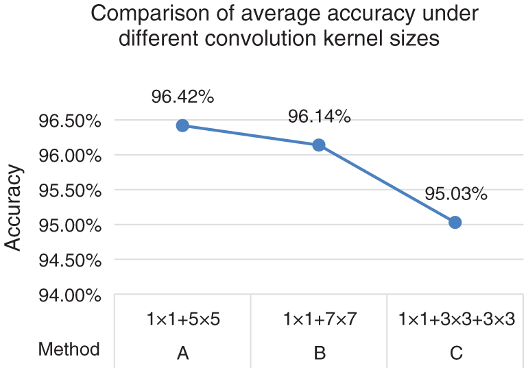
Figure 2: Comparison of average accuracy under different convolution kernel sizes

As indicated by Fig. 2, the combination methods of A, B in the third branch of the multi-size convolutional kernel module were more accurate than C combination, because a 3 × 3 convolutional kernel already existed in the 2nd and 4th branch, which verified that convolutional kernels of different sizes can extract features of different sizes and that richer feature information was beneficial to improve the classification accuracy. Among them, the average accuracy of A combination method was higher than that of B. This was because the tumor features on the MRI image were subtle, a small convolutional kernel was more suitable for extracting more useful information. According to the experimental results, this paper selects A combination method with the highest accuracy.

In order to determine the optimal method of adding dual-channel pooling layer, the following experiments are carried out under the condition that the multi-size convolution kernel module is determined as the combination method in method A in Fig. 2, which is carried out on the first cross validation scheme. Experiment 1: The average-pooling layer after Stage 5 in ResNet50 was kept unchanged, and only the max-pooling layer after Stage 1 was improved into dual-channel pooling layer. Experiment 2: The max-pooling layer after Stage 1 in ResNet50 was kept unchanged, and only the average-pooling layer after Stage 5 was improved into dual-channel pooling layer. Experiment 3: The single pooling layer after Stage 1 and Stage 5 were simultaneously improved into dual-channel pooling layer and the experimental results after such improvement are shown in Fig. 3.

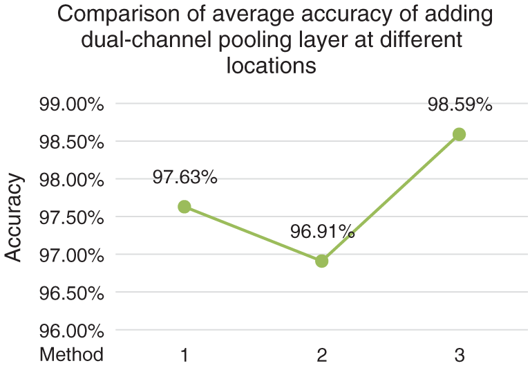
Figure 3: Comparison of average accuracy of adding dual-channel pooling layer at different locations

Fig. 3 shows that changing the max-pooling layer after Stage 1 into dual-channel pooling layer has a better classification effect than changing the average-pooling layer after Stage 5 into dual-channel pooling layer, which reflects that the average-pooling plays a more important role in complex brain tissue classification than max-pooling, and reveals the irreplaceability of global information in complex medical images. The experiment 3 changes the single pooling layer after Stage 1 and Stage 5 in the ResNet50 network into dual-channel pooling layer simultaneously, with a average classification accuracy reaching up to 98.59%, which indicates that the dual-channel pooling layer maximizes the advantages of max-pooling and average-pooling, and makes the high-dimensional feature information extracted by the two complement each other to make up for their respective shortcomings.

4.5 Performance Comparison of Training Set Before and After Data Enhancement Between ResNet50 and the Improved Network

In ResNet50 network and the improved network, two sets of experiments were carried out with two training sets before and after data enhancement, and the test set images were used as validation. The training set curve is drawn as shown in Fig. 4, where the dotted line represents the training curve without the operation of data enhancement. The experimental result is shown in Tab. 1.

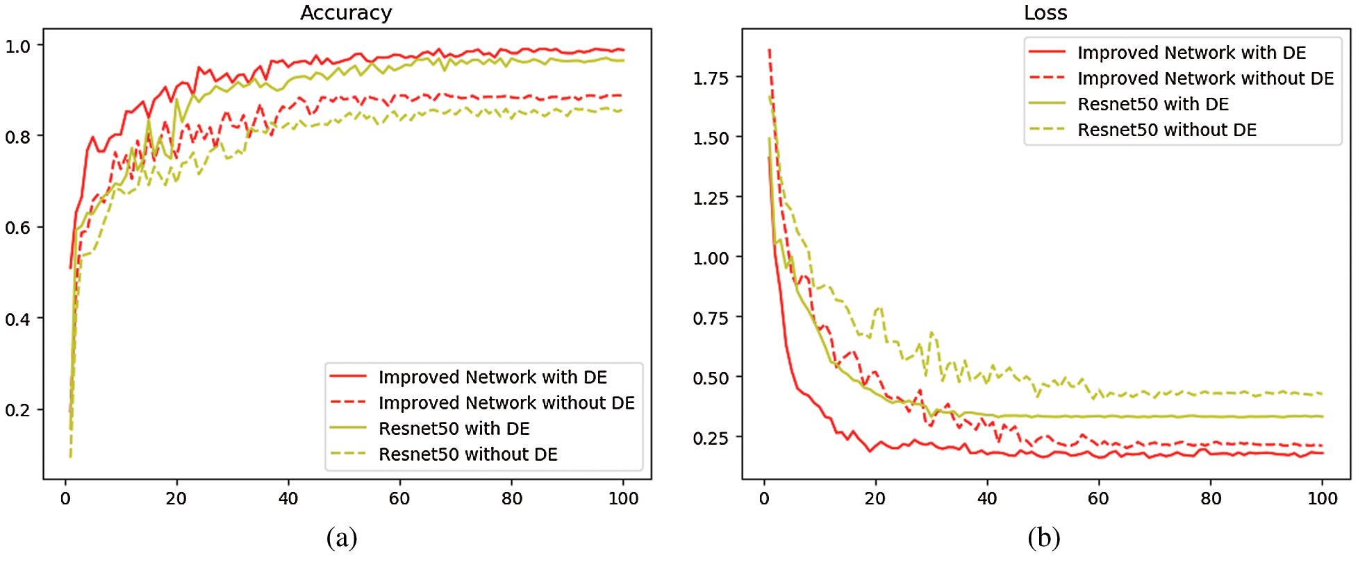
Figure 4: Comparison of the average accuracy and loss function of ResNet50 and improved network (a) Comparison of average classification accuracy between ResNet50 and improved network (b) Comparison of loss function decline between ResNet50 and improved network

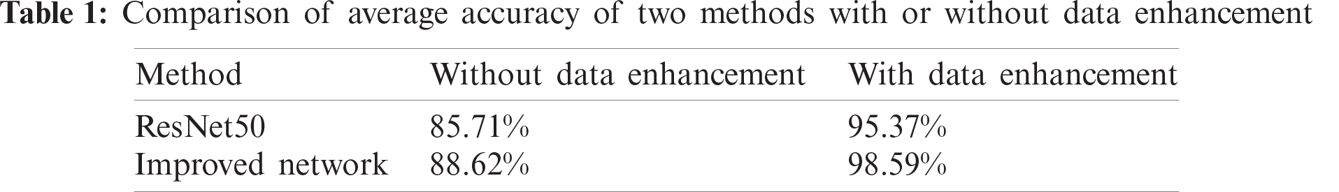
Tab. 1 and Fig. 4 show that, when the training set does not undergo data enhancement and is directly input into the network model for training, the average classification accuracy of ResNet50 network and the improved network is 85.71% and 88.62% respectively, while if the operation of data enhancement is performed on the training set, the average classification accuracy of ResNet50 is 95.37% and that of the improved network is 98.59%, both increasing by about 10%. This proves that the data enhancement technique has a positive impact on improving the classification accuracy. This is because the convolutional neural network requires a large amount of data to extract features and the stronger the ability of network learning features, the stronger the classification ability in the face of new datasets. At the same time, it is found that after 100 iterations, when the same small training sets are available, the average classification accuracy of the improved network is 2.91% higher than that of ResNet50 and the loss function is about 0.12 lower than that of ResNet50; when the same large training sets are available, the average classification accuracy of the improved network is 3.22% higher than that of the ResNet50, and the loss function is about 0.15 lower than that of the ResNet50, indicating that the features extracted by multi-size convolutional kernel module are richer than those extracted by the single convolutional layer, and that compared with the single pooling layer, the dual-channel pooling layer can combine the advantages of both max-pooling and average-pooling. All these are beneficial to improve the final classification performance. The above experimental results prove that the improvement based on ResNet50 is meaningful, and the improved network has better classification performance than ResNet50.

4.6 Comparison with Other Networks

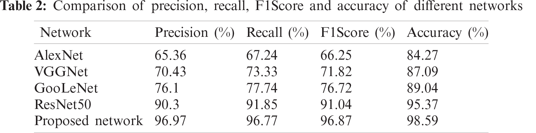
In order to verify the significance of the improvement of ResNet50, the experimental comparison between the improved network and AlexNet, VGGNet, GooleNet and ResNet50 is carried out. The experimental results are shown in Tab. 2, and the values in the table are classified average values.

The AlexNet model [26] is an eight-layer network. Its first five layers are convolutional layers, the last three are fully connected layers, and the last fully connected layer has 1000 classes of output. VGGNet is a 19-layer deep network model, including 16 convolutional layers, 2 fully connected image feature layers and 1 fully connected classification feature layer, and all convolutional kernels in the network are uniform in size, being 3 × 3. GooLeNet [20] is a 22-layer deep network model. Its biggest feature is the introduction of the inception structure, which solves the problem of large network parameters and high resource consumption. Five-fold cross-validation was performed on the training results of these five different network models. The following experimental result analysis is the average result of five validations.

It can be found from the above results that due to the close relationship between ResNet50 and the improved network, they can effectively solve the vanishing gradient problem by adding the residual module, which greatly reduces the number of parameters and increases the utilization of features. Both models outperform AlexNet, VGGNet and GoogLeNet in terms of precision, recall, F1Score and accuracy. Among them, AlexNet has the worst classification effect. However, the improved network has the highest results with regard to the four indices. The average classification precision of the improved network reaches 96.97%, and the average classification accuracy reaches 98.59%. The results show that the improved network can extract more features and it has effectively combined the advantages of max-pooling and average-pooling, so that the background information and the detail information extracted by the two can complement each other, thus the final recognition rate is relatively high.

5  Conclusions

For the multi classification of brain tumors, an improved convolutional neural network based on ResNet50 is proposed in this paper. The network uses multi-scale convolution core module and dual channel pooling layer to improve the single 7 × 7 convolution layer and single pooling layer in ResNet50. The multi size convolution core module is composed of convolution branches with different size convolution cores, which can extract rich feature information from the input image; the dual channel pooling layer combines the advantages of maximum pooling and average pooling, so that the extracted detail information and background information can complement each other. Accuracy, precision, recall and f1score were used to evaluate the network performance, and the five-fold cross validation method was used to analyze the classification effect of the network. Finally, the average classification accuracy of healthy brain, meningioma, diffuse astrocytoma, anaplastic oligodendroglioma and glioblastoma was 98.59%.

Acknowledgement: I would like to solemnly thank those who helped me generously in the process of my research. They are the instructors who give me pertinent suggestions on revision and the classmates who help me to collect dataset together. With their support and encouragement, I can successfully complete this paper.

Funding Statement: This paper is supported by the National Youth Natural Science Foundation of China (61802208), the National Natural Science Foundation of China (61873131), the Natural Science Foundation of Anhui (1908085MF207 and 1908085QE217), the Key Research Project of Anhui Natural Science (KJ2020A1215 and KJ2020A1216), the Excellent Youth Talent Support Foundation of Anhui(gxyqZD2019097), the Postdoctoral Foundation of Jiangsu (2018K009B), the Higher Education Quality Project of Anhui (2019sjjd81, 2018mooc059, 2018kfk009, 2018sxzx38 and 2018FXJT02), and the Fuyang Normal University Doctoral Startup Foundation (2017KYQD0008).

Conflicts of Interest: The authors declare that they have no conflicts of interest to report regarding the present study.

This work is licensed under a Creative Commons Attribution 4.0 International License, which permits unrestricted use, distribution, and reproduction in any medium, provided the original work is properly cited.