Computers, Materials & Continua DOI:10.32604/cmc.2021.018815
Article

Robust and Efficient Reliability Estimation for Exponential Distribution

Muhammad Aslam Mohd Safari1, Nurulkamal Masseran2,* and Muhammad Hilmi Abdul Majid2

1Department of Mathematics, Faculty of Science, Universiti Putra Malaysia, UPM Serdang, 43400, Selangor, Malaysia
2Department of Mathematical Sciences, Faculty of Science and Technology, Universiti Kebangsaan Malaysia, UKM Bangi, 43600, Selangor, Malaysia
*Corresponding Author: Nurulkamal Masseran. Email: kamalmsn@ukm.edu.my
Received: 22 March 2021; Accepted: 29 April 2021

Abstract: In modeling reliability data, the exponential distribution is commonly used due to its simplicity. For estimating the parameter of the exponential distribution, classical estimators including maximum likelihood estimator represent the most commonly used method and are well known to be efficient. However, the maximum likelihood estimator is highly sensitive in the presence of contamination or outliers. In this study, a robust and efficient estimator of the exponential distribution parameter was proposed based on the probability integral transform statistic. To examine the robustness of this new estimator, asymptotic variance, breakdown point, and gross error sensitivity were derived. This new estimator offers reasonable protection against outliers besides being simple to compute. Furthermore, a simulation study was conducted to compare the performance of this new estimator with the maximum likelihood estimator, weighted likelihood estimator, and M-scale estimator in the presence of outliers. Finally, a statistical analysis of three reliability data sets was conducted to demonstrate the performance of the proposed estimator.

Keywords: Exponential distribution; M-estimator; probability integral transform statistic; robust estimation; reliability

1  Introduction

Exponential distribution is the most widely used parametric distribution for modeling reliability and failure time data due to its mathematical simplicity and ability to create a realistic failure time model [1–5]. The advantages of applying a parametric model like exponential distribution in modeling failure time data are the following: this distribution can be concisely described with only one parameter instead of having to report an entire curve apart from providing smooth estimates of failure time distributions [1]. Besides the reliability analysis, the exponential distribution is also applied for modeling income distribution [6,7]. In the previous studies, research to propose a new model related to the family of exponential distributions has attracted considerable interest from many researchers [8–20]. The main objective of introducing an extension and modification to the exponential distribution is to offer more flexible distribution structures for fitting data.

Assume X as a random variable that follows the exponential distribution. Thus, the respective probability density function (PDF), cumulative distribution function (CDF), and survival function of the exponential distribution can be defined as follows:

f(x)=γe-γx,x>0,γ>0,(1)

F(x)=1-e-γx,x>0,γ>0,(2)

and

S(x)=1-F(x)=e-γx,x>0,γ>0,(3)

where γ is the rate or inverse scale parameter. A high value of γ indicates high risk and short survival while a low value of γ indicates low risk and long survival [3]. The parameter γ also measures the heaviness of exponential tail whereby the tail becomes heavier as γ decreases. In the analysis of reliability data, reliability properties are often defined using the mean time to failure (MTTF), survival (or reliability) function and failure rate function. Based on the exponential distribution, the survival function is given in Eq. (3), whereas the MTTF and failure rate function are expressed as the following:

MTTF=E[X]=1γ,x>0,γ>0,(4)

and

h(x)=f(x)S(x)=γ,γ>0.(5)

The reliability data can be sometimes contaminated with outliers. Outliers are observations much deviated from the bulk of the data [21] and are also referred to as abnormalities, discordants, deviants, or anomalies in statistics literature [22]. Outliers may arise due to errors or simply by natural deviations in a data set. In statistical modeling using parametric distribution, the classical estimator known as maximum likelihood estimator (MLE) is the most commonly used method for estimating the parameters of any parametric model. In fact, for any typical parametric distribution, MLE is well known to be efficient especially for a large sample size. However, in the presence of data contamination in which the outliers are present in the data set, the MLE is not robust and severely biased [23]. Consequently, this condition may affect the application of exponential model in reliability analysis or any assessment. Therefore, when the outliers are present, a robust estimator should be utilized for estimating the parameter of any parametric distribution as an alternative to the MLE.

Several robust methods have been proposed in the literature for estimating the parameter of exponential distribution. Thall [24] proposed a robust estimator for the parameter of exponential distribution called Huber-sense robust M-estimator. However, this estimator is only suitable for the case when the proportion of outliers is small. Trimmed-mean and Winsorized-mean type estimators have also been proposed and studied by several researchers [25–27]. The advantage of these types of estimator is that they are simple to compute. Further, Gather et al. [28] proposed another simple robust estimator called standardized median estimator (SME). However, the SME has low asymptotic relative efficiency (ARE) of only 48%. Gather et al. [28] also compared the performance of SME with two other estimators called RCS-estimator and RCQ-estimator in which the respective AREs for both estimators were 55% and 74%. Meanwhile, Ahmed et al. [29] introduced another robust estimator called the weighted likelihood estimator (WLE). When estimating the parameter of exponential distribution using WLE, observations with small likelihood are assigned with zero weights. This procedure causes the outliers to be eliminated from the data set and then, the ordinary MLE is used to estimate the parameter of interest based on the remaining observations. In recent years, Shahriari et al. [23] proposed a robust M-scale estimator for the parameter of exponential distribution in which this estimator has a maximum ARE of 71%. This estimator uses families of bisquare function as the weight for estimating the parameter of interest.

This study aims to develop a new robust estimator for the parameter of exponential distribution based on the probability integral transform statistic, which offers reasonable protection against outliers. Generally, probability integral transform statistic is used to transform the random variable of any continuous distribution to a standard uniform distribution [30–32]. It should be noted that the new robust estimator proposed in this study is a class of M-estimator. This estimator has a simple form and easy to compute. In this study, the robustness of this new estimator was examined based on the measures of asymptotic variance, breakdown point, and gross error sensitivity.

The rest of this paper is structured as follows. Section 2 provides a brief explanation of M-estimators and then presents the new robust estimation method for the rate parameter of exponential distribution. Section 3 compares the performance of the proposed estimator with several estimators in the presence of outliers through a simulation study. Section 4 applies the proposed method for estimating the rate parameter of exponential distribution to real data sets. Finally, Section 5 concludes the paper.

2  Proposed Estimator

In this section, a brief explanation of the M-estimators is given followed by the introduction of the new estimator developed based on the probability integral transform statistical approach. Furthermore, the robustness of this new estimator was compared with the ordinary MLE and discussed in this section.

2.1 M-Estimators

M-estimators are generalized ML estimators that provide tools for measuring the robustness of the maximum likelihood-type estimates. As described in Huber [33], an estimator βn defined by

βn= argminβ∑i=1nρ(xi,β)(6)

or

∑i=1nψ(xi,βn)=0(7)

is known as an M-estimator. ρ is a measurable function on X×Θ and ψ(x,β)=(∂/∂β)ρ(x,vβ) denotes the derivative of the function ρ with respect to β (when it exists). Note that if ρ(x,β)=-logf(x;β), then β^n is the ordinary MLE. Let x1,x2,…,xn be a random sample from an exponential distribution as described in (2). The MLE for parameter γ is given by

γ^MLE=n∑i=1nxi.(8)

2.2 Probability Integral Transform Statistic Estimator

Assume that x1,x2,…,xn is a random sample from the exponential distribution. Since the CDF of exponential distribution in Eq. (2) is continuous and strictly increasing, the random variables F(x1),F(x2),…,F(xn) follow a standard uniform distribution, which is F(X)~Unif(0, 1). Define

Hn,κ(β)=n-1∑i=1ne-βκxi,(9)

where κ>0 denotes a tuning parameter to be used in regulating the balance between efficiency and robustness. When β=γ and κ=1, e-γxi=S(xi)=1-F(xi), is a random variable that follows the standard uniform distribution. Suppose that u1,u2,…,un is a random sample from a standard uniform distribution. According to the strong law of large numbers, n-1∑i=1nuiκ converges to E[Uκ]=1/(κ+1) as n→∞ with probability 1. Thus, the probability integral transform statistic estimator (PITSE) of parameter γ^ is defined as the solution of the following equation:

Hn,κ(β)=n-1∑i=1ne-βκxi=1κ+1.(10)

Note that Eq. (10) can be solved using any numerical method such as bisection, secant, or Newton–Raphson method.

Lemma 1. For any fixed κ>0, the equation Hn,κ(β)=1/(κ+1) in (10) has exactly one solution.

Proof of Lemma 1. Note that Hn,κ(β) is continuous on [0, ∞) and that Hn,κ(0)=1>1/(κ+1) while limβ→∞Hn,κ(β)=0<1/(κ+1). Based on the intermediate value theorem, Hn,κ(β)=1/(κ+1) for some β in [0, ∞). That is, Eq. (10) has at least one solution. Then, it can be shown that Hn,κ′(β)=-n-1∑i=1nκxie-βκxi<0 for all β>0. Thus, Hn,κ(β) is strictly monotonic with respect to β and it can be concluded the Eq. (10) has a unique solution.

The PITSE for the rate parameter of exponential distribution is a class of M-estimator with

ψ(x;β)=e-βκx-1κ+1.(11)

To investigate the properties of PITSE, the function introduced by Huber [33] can be utilized as follows:

λ(β)=∫0∞ψ(x;β)f(x)dx.(12)

Thus, based on Eq. (12), the following is obtained:

λ(β)=κ(γ-β)(βκ+γ)(κ+1).(13)

Theorem 1. For any fixed κ>0, the PITSE γ^PITSE converges to γ as n→∞ with probability 1.

Proof of Theorem 1. Based on Proposition 2.1 and Corollary 2.2 in Chapter 3 of Huber [33], λ(β)>0 for β<γ and λ(β)<0 for β>γ. As the PITSE is uniquely defined, γ^PITSE is a consistent estimator of γ.

2.3 Efficiency of PITSE

The MLE is well known to be efficient in the sense that it has minimum asymptotic variance. For this reason, MLE is useful in providing a quantitative benchmark on the measure of efficiency. Note that the MLE for the rate parameter given in Eq. (8) is asymptotically normal with a mean γ and variance γ2/n, i.e., γ^MLE~N(γ,γ2/n). The asymptotic distribution γ^PITSE is given in Theorem 2.

Theorem 2. For any fixed κ>0, the estimator n(γ^PITSE-γ) is asymptotically normal with mean 0 and variance γ2(κ+1)2/(2κ+1), i.e., γ^PITSE~N(γ,γ2(κ+1)2/[n(2κ+1)]).

Proof of Theorem 2. Based on Corollary 2.5 in Chapter 3 of Huber [33], λ′(γ)=-κ/[γ(κ+1)2] and σ02=∫0∞ψ(x;γ)2f(x)dx-λ(γ)2=κ2/[(2κ+1)(κ+1)2]. Therefore, the asymptotic variance of γ^PITSE is σ02/[λ′(γ)]2=γ2(κ+1)2/(2κ+1). Note that for the finite sample, the variance of γ^PITSE is γ2(κ+1)2/[n(2κ+1)].

The ARE of PITSE is defined as the ratio of the asymptotic variance of the MLE to the asymptotic variance of the PITSE. In other words, the ARE measures the relative efficiency of the estimator γ^PITSE compared with γ^MLE. The ARE of PITSE for parameter γ is given by

ARE=Var(γ^MLE)Var(γ^PITSE)=2κ+1(κ+1)2.(14)

As the value of κ increases, the value of ARE decreases. In other words, when the value of κ increases, the PITSE gains robustness but with its relative efficiency reduced. By taking κ close to 0, ARE of PITSE can be made arbitrarily close to 1. The guidelines for choosing suitable ARE of PITSE in practical application are given in the simulation study section.

2.4 Breakdown Point of PITSE

The breakdown point (BP) is a useful measure of the robustness of a statistical approach in which the degree of sensitivity of an estimator to data contamination is measured. According to Huber [34], BP is defined as the largest contamination proportion that can be tolerated by an estimator before breaking down. A higher value of BP is an indication that an estimator is more robust against data contamination. In general, two types of BP exist; lower breakdown point (LBP) and upper breakdown point (UBP). In the present context of γ estimation, LBP is the largest proportion of lower contamination that can be tolerated by an estimator before forcing γ^→∞. On the other hand, the UBP is the largest proportion of upper contamination that can be tolerated by an estimator before forcing γ^→0. Since the contamination of the upper-end of the distribution is crucial in typical applications, only the UBP was emphasized in this study.

Note that the MLE, namely γ^MLE, has a UBP equal to 0 because the function ψ(x;γ^MLE)=1/γ^MLE-x is unbounded in x. For the finite sample, if a single observation xi→∞, then ∑i=1nxi→∞ and consequently, γ^MLE→0. This result shows that even an extreme value of single contaminated data in the upper tail of the observations could contribute to the unreliable performance of γ^MLE. The UBP and LBP of PITSE are given in Theorem 3.

Theorem 3. The respective UBP and LBP of PITSE are κ/(κ+1) and 1/(κ+1). For the finite sample, the UBP and LBP of PITSE are ⌈nκ/(κ+1)⌉/n and ⌈n/(κ+1)⌉/n, respectively.

Proof of Theorem 3. For any integer 1≤m≤n, the estimator γ^PITSE is defined as n-1∑i=1me-κxiγ^PITSE+n-1∑i=m+1ne-κxiγ^PITSE=1/(κ+1). Suppose that x1,x2,…,xm take on values that approach ∞. Certainly, n-1∑i=m+1ne-κxiγ^PITSE=1/(κ+1)<(n-m)/n because the term e-κxiγ^PITSE is less than 1. This solution is valid if and only if 1/(κ+1)<(n-m)/n, that is, m<nκ/(κ+1). Thus, the finite sample UBP is ⌈nκ/(κ+1)⌉/n, where ⌈⋅⌉ is the ceiling function. By taking n→∞ in the finite sample UBP, UBP equal to κ/(κ+1) will be obtained. Similarly, let x1,x2,…,xm take on values approaching 0. it can be shown that m/n+n-1∑i=m+1ne-κxiγ^PITSE=1/(κ+1). This solution is finite if and only if 1/(κ+1)>m/n, that is, m<n/(κ+1). Therefore, the finite sample LBP is ⌈n/(κ+1)⌉/n, and by letting n→∞, the LBP will be equal to 1/(κ+1).

2.5 Gross Error Sensitivity of PITSE

The breakdown point (BP) is a useful measure of the robustness of a statistical approach in which the degree of sensitivity of Gross error sensitivity (GES) is also an important measure of the robustness of an estimator. According to Hampel et al. [35], GES is the supremum of the absolute value of the influence function (IF). The IF of an estimator βn that satisfies Eq. (7) can be defined by the following:

IF(x;ψ,F)=-ψ(x,β(F))∫(∂/∂γ)[ψ(y,γ)]β(F)dF(y),(15)

where β(F) denotes the solution βn of Eq. (7) with samples generated from the CDF F. Then, the GES is given by

GES= supx|IF(x;ψ,F)|,(16)

An estimator with small GES should be more robust than that with larger GES. The MLE, which is γ^MLE, has an infinite GES because ψ(x;γ^MLE) is an unbounded function. This result proves that MLE is a non-robust estimator. Then, the GES of PITSE is provided in Theorem 4.

Theorem 4. The GES of the PITSE is max{γ(κ+1)/κ,γ(κ+1)}.

Proof of Theorem 4. By applying the formula of IF in Eq. (15), the IF of PITSE can be demonstrated as IF(x;ψ,F)=-ψ(x;γ)γ(κ+1)2/κ. As ψ(x; γ) is monotone in x, the maximum value occurs when either x→∞ or x→0. Note that ψ(x;γ)=-1/(κ+1) when x→∞ and ψ(x;γ)=κ/(κ+1) when x→0. Then, using the formula in Eq. (16), the GES of PITSE is obtained.

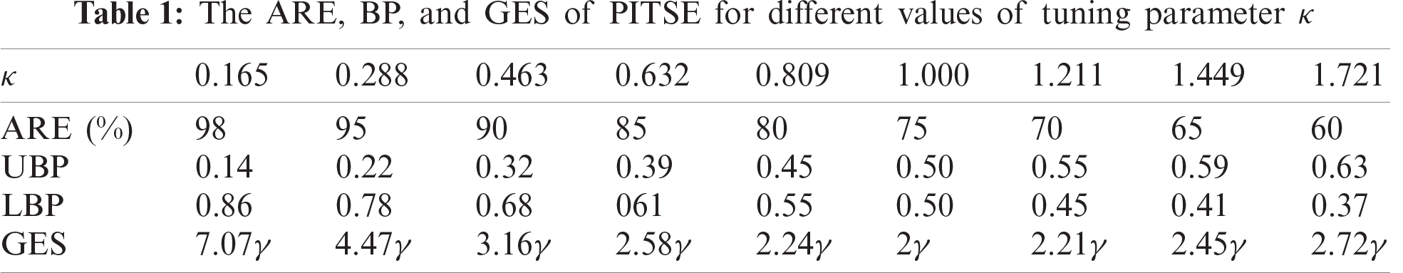
Tab. 1 shows the properties of the PITSE based on ARE, BP, and GES for different values of tuning parameter κ. The properties of the PITSE can be summarized as follow:

•   As the value of κ increases, the PITSE loses efficiency (ARE decreases) but also becomes more resistant to upper contamination.

•   As the value of κ increases, the UBP increases, and the LBP, which suggests that the robustness of the PITSE, increases against upper contamination. On the other hand, the LBP decreases as the value of κ increases, which indicates that the robustness of the PITSE decreases against lower contamination.

•   As the value of κ increases up to 1, the GES of the PITSE decreases. But then, the GES of the PITSE started to increase when the value of κ is greater than 1.

3  Simulation Study

In this section, a simulation study to compare the performance of the MLE, PITSE, WLE, and M-scale estimator in the presence of outliers is conducted. The design and results of the simulation study are given in the next two following subsections. Then, the guidelines for selecting the suitable ARE of the PITSE for practical application purposes are provided.

3.1 Design of Simulation

In the simulation study, the methods considered for comparison were MLE, PITSE (90% and 70% ARE), WLE (90% and 70% ARE), and M-scale estimator (70% ARE). The data sets were simulated from an exponential distribution, Exp(γ), with different values of rate parameter, γ=0.5, 1, 1.5, and 2. The sample size used in this simulation study was divided into two cases: small sample sizes (n=30, 50, and 70) and large sample sizes (n=100, 300, and 500). Then, some observations in the data sets were randomly selected and replaced with outliers. According to Lin et al. [36], the observations are from exponential distribution with parameter ωγ, which is Exp(ωγ) with 0<ω<1 considered as outliers. Thus, in this simulation study, the outliers were generated from an exponential distribution with parameter 0.05γ, which was Exp(0.05γ). For the case of small sample sizes, the outliers were generated from Exp(0.05γ) for several fixed numbers, k=1, 3, and 5. For the case of large sample sizes, the outliers were simulated from Exp(0.05γ) for several fixed proportions, ε=1%, 5%, and 10%. This simulation was repeated for 10,000 data sets found based on 10,000 simulation runs.

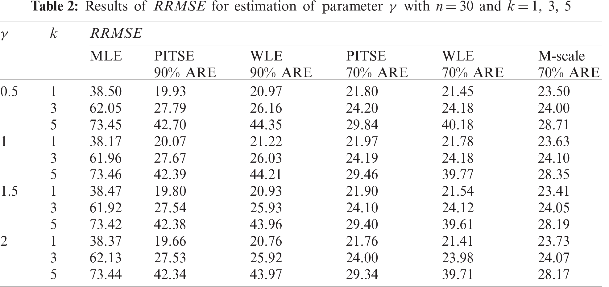
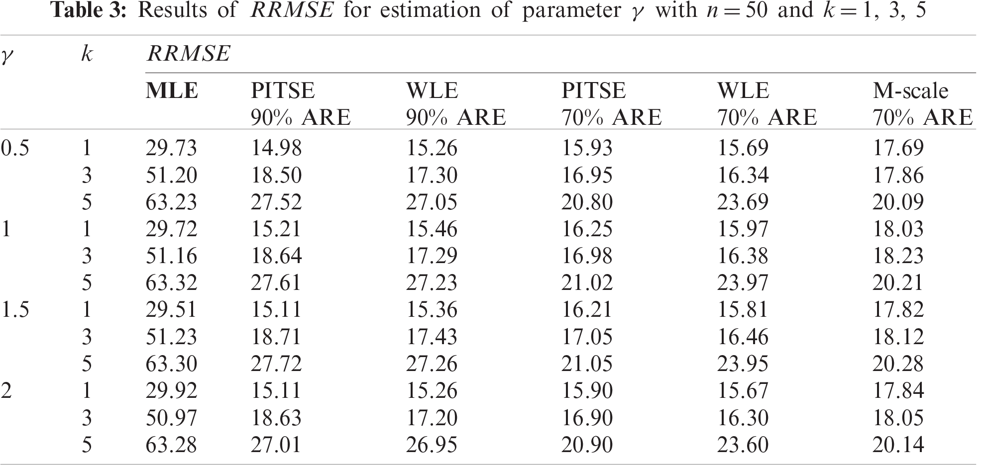
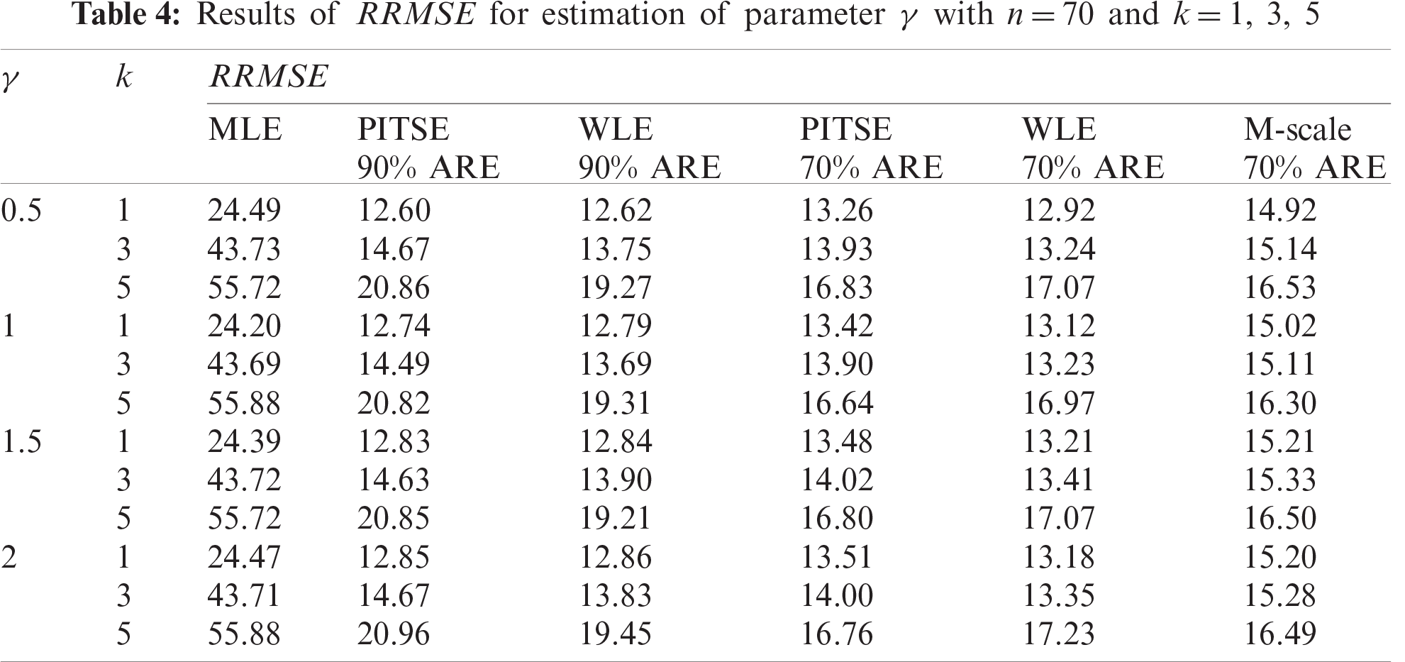
The performance of the estimators was assessed in terms of percentage relative root mean square error (RRMSE). For a given true value of the rate parameter of exponential distribution, γ, the RRMSE is given by

RRMSE=100γ1N∑i=1N(γ^i-γ)2,(17)

where γ^i is the estimated rate parameter for the i-th (i=1,2,…,N) simulated data, and N is the number of simulations. A smaller value of RRMSE indicates that the estimator is more accurate and precise. Therefore, the estimation method that minimizes the RRMSE was considered to be the best for estimating the rate parameter γ in the presence of outliers.

3.2 Results of Simulation

Results based on the simulation study are presented in Tabs. 2–7. For the case of small sample sizes, when n=30 and k=1, for all values of the parameter γ, the value of RRMSE found for PITSE and WLE with 90% ARE were nearly similar and smaller than those for other estimators as shown in Tab. 2, indicating that these two estimators performed better than other estimators for this particular case. Furthermore, from Tab. 2, when the number of outliers increased to k=3, the PITSE, WLE, and M-scale estimator with 70% ARE performed almost equally and outperformed other estimators due to smaller values of RRMSE. When k=5, it was observed that the PITSE and M-scale estimator with 70% ARE performed almost equally and outperformed other estimators as presented in Tab. 2. As the sample size increases, the performance of all estimators improves for all cases considered because the values of RRMSE became smaller as shown in Tabs. 2–4. For all cases of small sample sizes, the MLE produced a high value of RRMSE, indicating a poor performance of this method when the outliers were present in the data set.

The simulation results for the case of large sample sizes are shown in Tabs. 5–7. Based on Tab. 5, for n=100, the PISTE and WLE with 90% and 70% ARE performed almost equally and outperformed other estimators in the case of a small degree of contamination, where ϵ=1%. When the degree of contamination increased to moderate, which was ϵ=5% the PITSE, WLE, and M-scale estimator with 70% ARE produced much better performance than other estimators. At a high degree of contamination where ϵ=10%, the PITSE and M-scale estimator with 70% ARE performed almost equally and outperformed other estimators. Although WLE is a robust estimator, it performed substantially worse than the PITSE and the M-scale estimator in the case of a high degree of contamination. The reason is that a large proportion of observations (outliers) in the data set was not being considered, which reduced the sample size and, consequently causing the efficiency of the WLE to be decreased. As shown in Tabs. 5–7, when the sample size increases, the performance of all estimators improves. However, similar to the case of small sample size, the performance of MLE was also poor when outliers were present in the data set for the case of large sample size. Thus, the use of the MLE for estimating the parameter γ should be avoided since this estimator does not protect outliers even in the small degree of contamination.

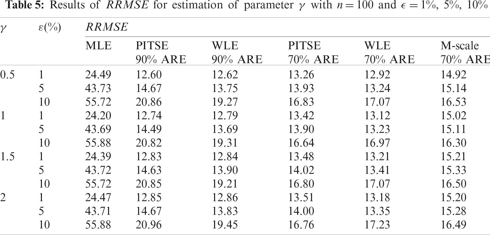
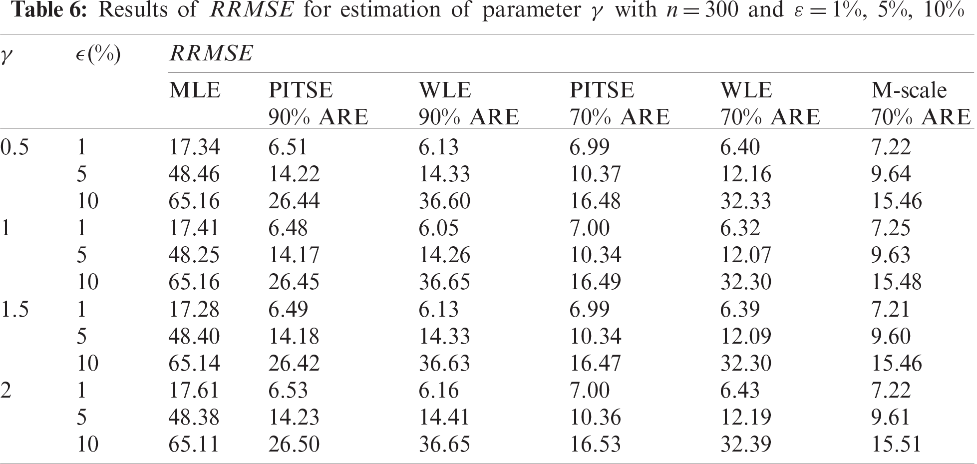
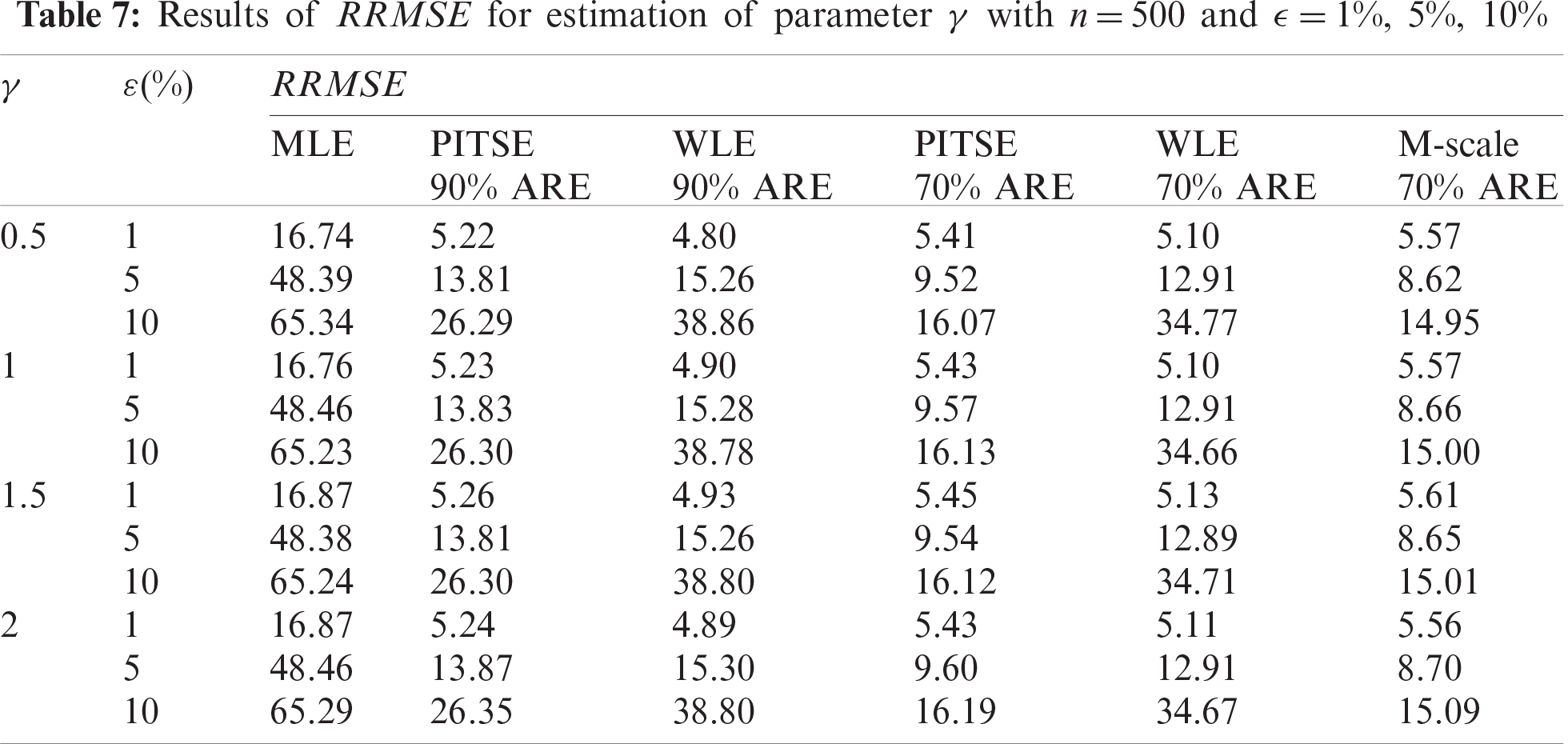
3.3 Guidelines for Selecting Suitable ARE of PITSE in Practical Application

In practice, the suitable ARE of PITSE can be selected based on sample size and number or proportion of outliers. Based on a comprehensive simulation study, the guidelines for selecting the suitable ARE of PITSE in practical application are provided in Tab. 8.

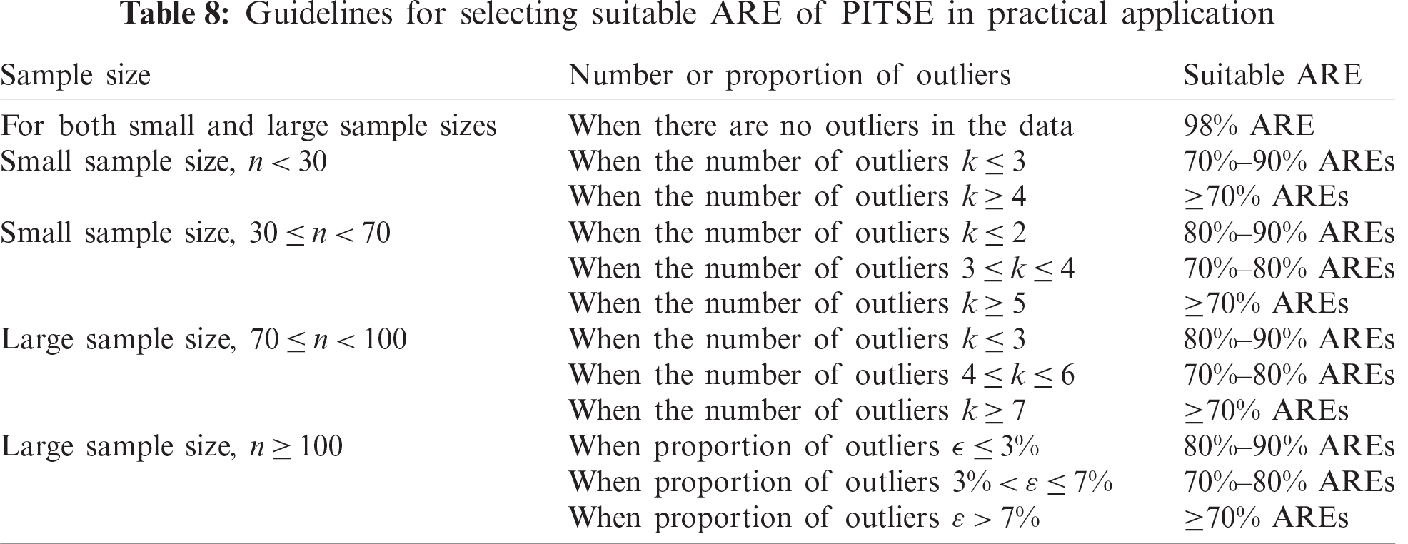
It should be noted that when there are a large number or proportion of outliers in a data set, PITSE with ARE not less than 60% should be used to make sure that the PITSE has a reasonable efficiency in estimating the rate parameter of exponential distribution.

4  Application on Reliability Data Sets

In this section, three applications of exponential distribution are proposed using three real data sets to compare the performance of MLE, PITSE, WLE, and M-scale estimator. This comparative study considered several ARE levels for PITSE and WLE, while a fixed ARE level of 70% was used for the M-scale estimator. The first data set (Set 1) was obtained from Linhart et al. [37], which represents the failure times of the air-conditioning system of an airplane. The second data set (Set 2) consisted of the reliability data of a 180-tonne rear dump truck obtained from Badr et al. [38]. Lastly, the third data set (Set3) was obtained from Proschan [39] consisting of the number of successive failures for the air conditioning system of each member in a fleet of 13 Boeing 720 jet airplanes. The pooled data, yielding a total of 213 observations, have also been analyzed by other authors such as Kuş [40] and Tahmasbi et al. [8]. All the data sets used are given in Appendix A.

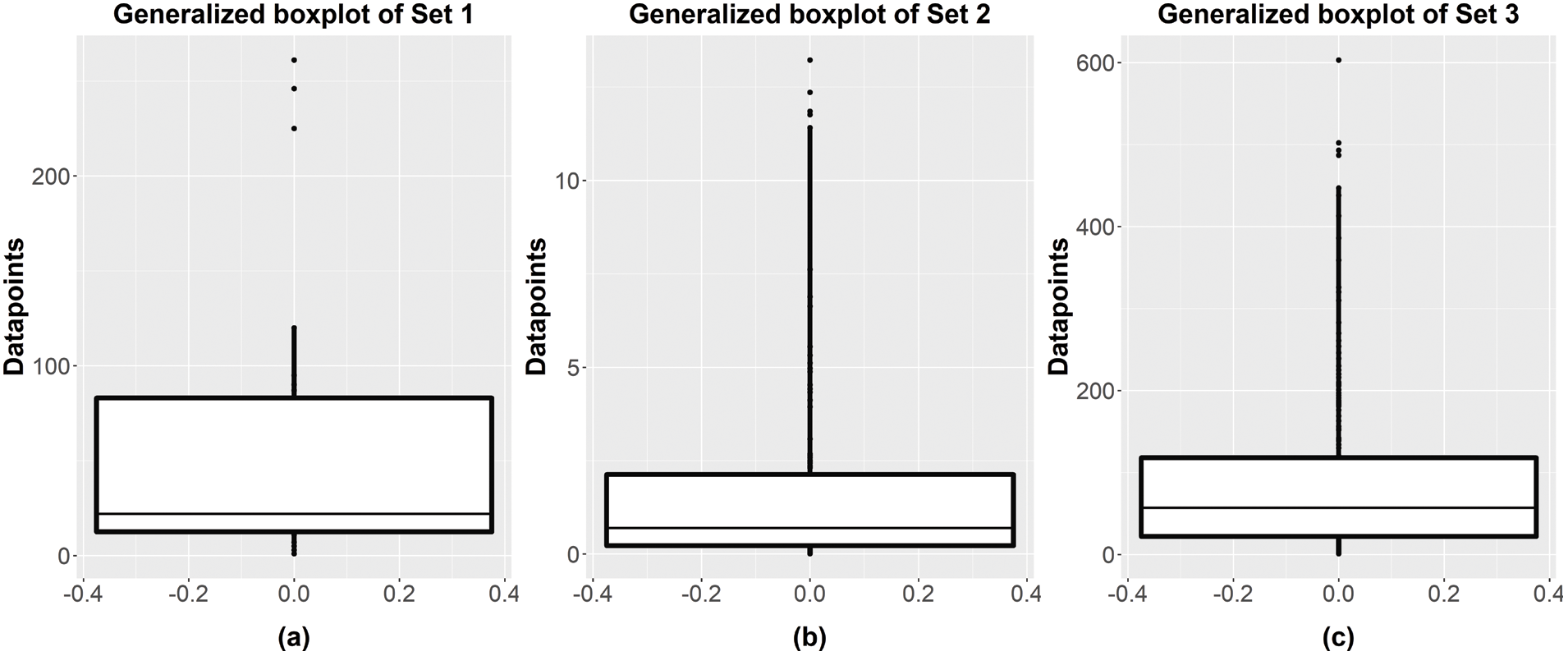
Figure 1: Generalized boxplot for data (a) Set 1, (b) Set 2 and (c) Set 3

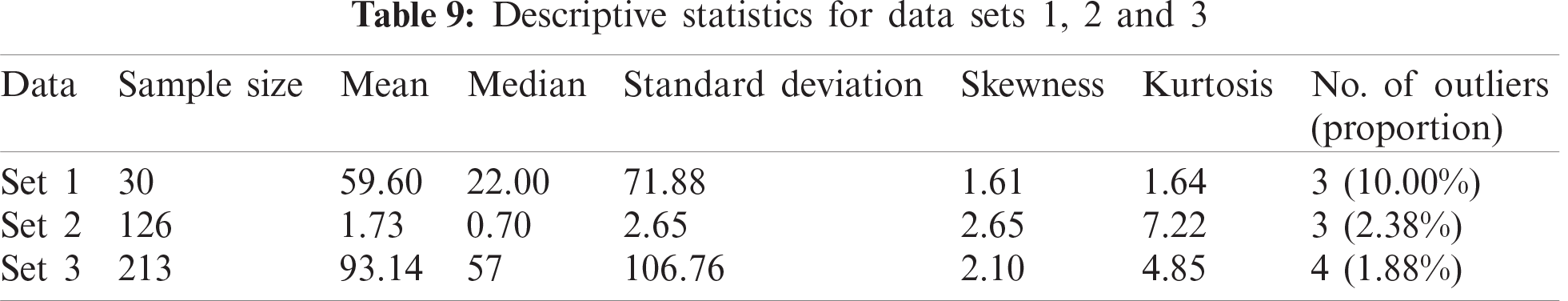
To identify the presence of outliers in all data sets, the generalized boxplot method [41], which is suitable for skewed and/or heavy-tailed distributions, was utilized. According to Bruffaerts et al. [41], this boxplot relies on a simple rank-preserving transformation that allows the data to fit a Tukey g-and-h distribution. It was found that the generalized boxplot was robust against outliers and has clear advantages over the standard boxplot particularly for the case of skewed and/or heavy-tailed distributions. Fig. 1 shows the generalized boxplot for all considered data sets, while Tab. 9 presents the descriptive statistics of these data sets.

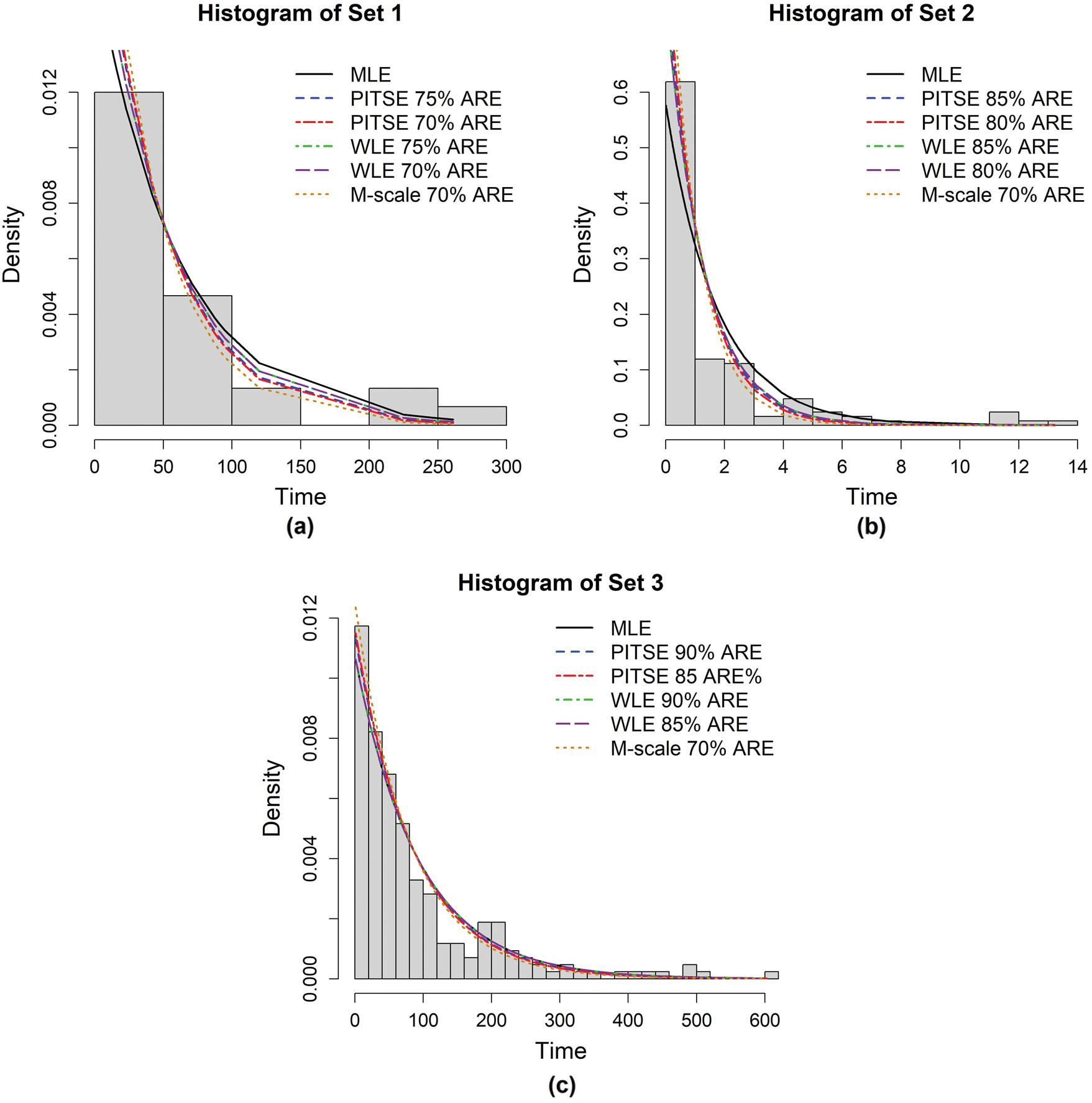
Figure 2: Fitted exponential densities on the histograms of data (a) Set 1, (b) Set 2 and (c) Set 3 based on several different estimators

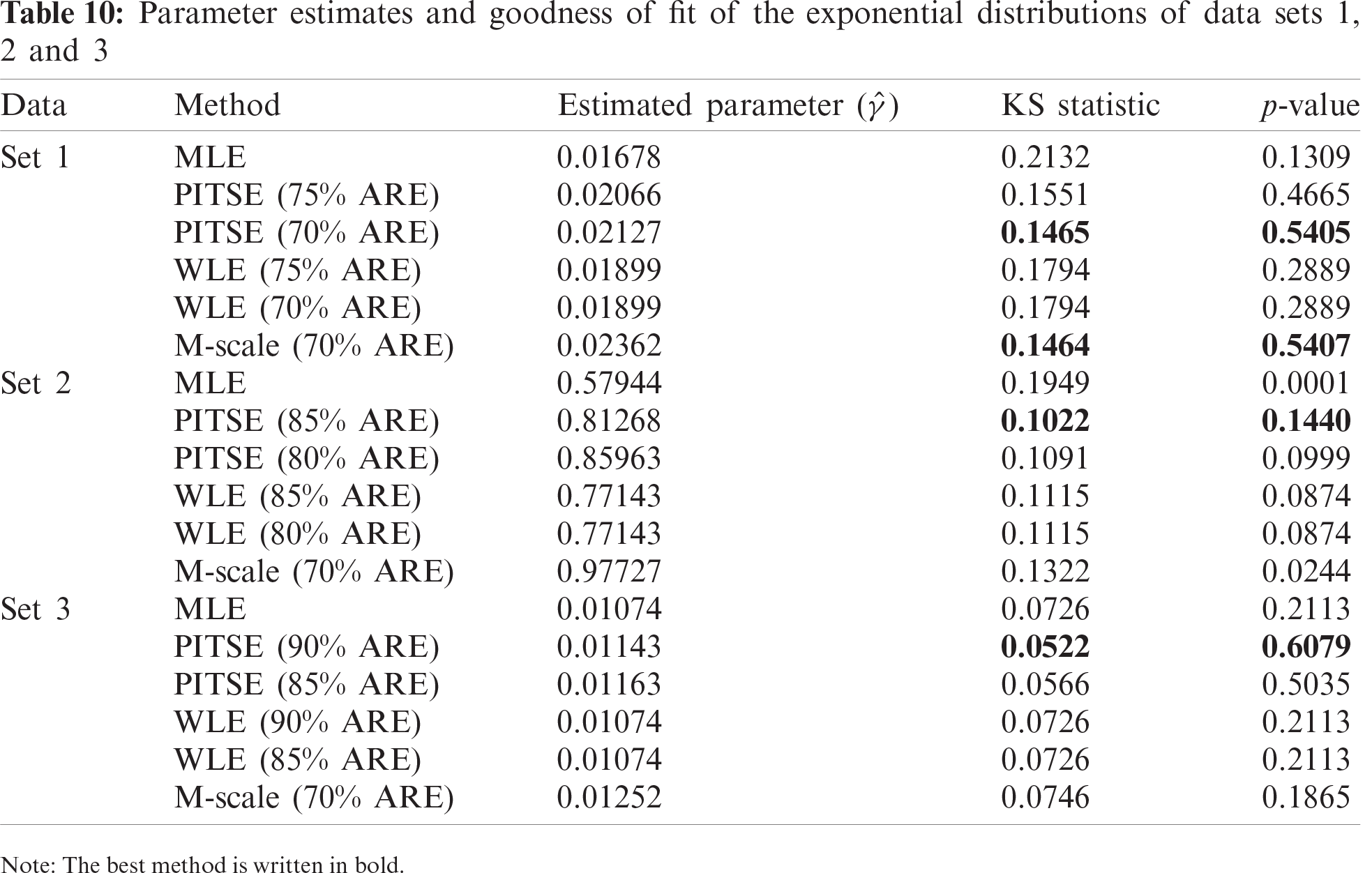
To compare the performance of all considered methods in estimating the parameter of exponential distribution, the Kolmogorov–Smirnov (KS) tests were employed as a goodness-of-fit assessment. The best method was determined by choosing the smallest values of KS statistics as well as the highest p-values of the KS test. Tab. 10 reports the estimated parameter and goodness-of-fit of the exponential model for all data sets. For data Set 1, it can be observed that the PITSE (70% ARE) and M-scale estimator (70% ARE) performed almost equally and provided a better estimation of exponential parameter compared to other methods based on their smallest KS statistic and highest p-value of the KS test. For data Set 2, the PITSE has outperformed other methods in estimating the rate parameter. It can be also seen for data Set 2 that the MLE and M-scale estimators failed to provide a good estimation of rate parameters based on the small value of the KS test found for these two estimators. For data Set 3, the PITSE was found to be the best method to estimate the rate parameter. Nevertheless, other methods were also found quite reliable for estimating the rate parameter based on the reasonable p-value of KS test (p-value ¿ 0.05). Fig. 2 demonstrates the fitted exponential density on the histogram of each data set based on several different estimators.

Since the measures of reliability based on the exponential distribution depend on the parameter γ, it is crucial to employ the appropriate method for estimating parameter γ. Based on the simulation study and its application to real data sets, it was demonstrated that the proposed PITSE can represent a viable alternative for estimating the rate parameter of the exponential distribution, particularly for the case when outliers are present in the data.

5  Conclusion and Discussion

In this study, a robust and efficient estimator for the parameter of exponential distribution called PITSE has been introduced based on probability integral transform statistic. The asymptotic variance, BP, and GES were derived to study the PITSE properties. The advantage of PITSE is that it is conceptually simple and easy to compute. According to the simulation study, PITSE performed better than MLE and was comparable with WLE and M-scale estimator when outliers are present in the data set. However, in the case of a high degree of contamination, the performance of WLE was worse than PITSE and M-scale estimator. On the other hand, the M-scale estimator only has the maximum ARE of about 71%, which makes it unsuitable for estimating the parameter of exponential distribution in the case of a small degree of contamination. Therefore, the PITSE introduced in this study was considered a viable alternative for estimating the parameter of exponential distribution in the presence of outliers. Finally, the application on three real data sets showed that the PITSE provided desirable protection against outliers. The R commands for PITSE are available in Appendix B.

Although the PITSE proposed in this study was considered viable for estimating the exponential parameter, there existed a limitation regarding the scope of the current work. It was the reliability modeling under exponential model assumptions that was limited to certain cases (constant failure rate) since the exponential distribution is a simple model consisting of one parameter. There are two-parameter distributions such as Weibull that could provide a better fit to the reliability data, hence providing a better reliability estimation. Therefore, for future work, the robust and efficient estimator for the Weibull parameters can be developed based on the probability integral transform statistical approach. From there, it is believed that a better reliability estimation can be obtained particularly for the case when the outliers are present in the data set.

Acknowledgement: The authors would like to thank the editor for the time spent reviewing this manuscript.

Funding Statement: This work is supported by the Universiti Kebangsaan Malaysia [Grant Number DIP-2018-038].

Conflicts of Interest: The authors declare that they have no conflicts of interest to report regarding the present study.

Appendix A. Data Sets 1, 2 and 3

Set 1:

23, 261, 87, 7, 120, 14, 62, 47, 225, 71, 246, 21, 42, 20, 5, 12, 120, 11, 3, 14, 71, 11, 14, 11, 16, 90, 1, 16, 52, 95

Set 2:

0.01, 0.01, 0.01, 0.01, 0.01, 0.02, 0.02, 0.02, 0.02, 0.03, 0.04, 0.06, 0.08, 0.1, 0.1, 0.12, 0.12, 0.12, 0.13, 0.14, 0.15, 0.15, 0.15, 0.16, 0.16, 0.17, 0.18, 0.18, 0.19, 0.2, 0.21, 0.22, 0.23, 0.25, 0.26, 0.28, 0.28, 0.3, 0.32, 0.34, 0.36, 0.38, 0.39, 0.41, 0.41, 0.42, 0.43, 0.44, 0.44, 0.45, 0.45, 0.5, 0.53, 0.56, 0.58, 0.58, 0.61, 0.62, 0.62, 0.62, 0.64, 0.66, 0.7, 0.7, 0.7, 0.72, 0.77, 0.78, 0.78, 0.8, 0.82, 0.83, 0.85, 0.86, 0.96, 0.97, 0.98, 0.99, 1.05, 1.06, 1.07, 1.18, 1.35, 1.36, 1.42, 1.55, 1.59, 1.65, 1.73, 1.77, 1.79, 1.8, 1.91, 2.09, 2.14, 2.15, 2.15, 2.31, 2.33, 2.36, 2.43, 2.45, 2.5, 2.51, 2.58, 2.64, 2.68, 3.08, 3.94, 4.12, 4.33, 4.42, 4.53, 4.88, 4.97, 5.11, 5.32, 5.55, 6.63, 6.89, 7.62, 11.41, 11.76, 11.85, 12.36, 13.22

Set 3:

194, 15, 41, 29, 33, 181, 413, 14, 58, 37, 100, 65, 9, 169, 447, 184, 36, 201, 118, 34, 31, 18, 18, 67, 57, 62, 7, 22, 34, 90, 10, 60, 186, 61, 49, 14, 24, 56, 20, 79, 84, 44, 59, 29, 118, 25, 156, 310, 76, 26, 44, 23, 62, 130, 208, 70, 101, 208, 74, 57, 48, 29, 502, 12, 70, 21, 29, 386, 59, 27, 153, 26, 326, 55, 320, 56, 104, 220, 239, 47, 246, 176, 182, 33, 15, 104, 35, 23, 261, 87, 7, 120, 14, 62, 47, 225, 71, 246, 21, 42, 20, 5, 12, 120, 11, 3, 14, 71, 11, 14, 11, 16, 90, 1, 16, 52, 95, 97, 51, 11, 4, 141, 18, 142, 68, 77, 80, 1, 16, 106, 206, 82, 54, 31, 216, 46, 111, 39, 63, 18, 191, 18, 163, 24, 50, 44, 102, 72, 22, 39, 3, 15, 197, 188, 79, 88, 46, 5, 5, 36, 22, 139, 210, 97, 30, 23, 13, 14, 359, 9, 12, 270, 603, 3, 104, 2, 438, 50, 254, 5, 283, 35, 12, 130, 493, 100, 7, 98, 5, 85, 91, 43, 230, 3, 130, 230, 66, 61, 34, 487, 18, 14, 57, 54, 32, 67, 59, 134, 152, 27, 14, 102, 209

Appendix B. R Commands for PITSE

### PITSE for the rate parameter ###

f < -function(data,l,k){

n < -length(data)

fx < -(sum(exp( − l * k * data))/n) − (1/(k + 1))

return(fx)

}

#solve using secant method

# k – tuning parameter

# l1 – 1st initial value; l2 − 2nd initial value

pitse < -function(data,k, l1, l2, num = 1000, eps = 1e-05, eps1 = 1e-05)

{

i = 0

while ((abs(l1 - l2) > eps) && (i < num)) {

c = l2 − f(data,l2,k) * (l2 − l1)/(f(data,l2,k) − f(data,l1,k))

l1 = l2

l2 = c

i = i + 1

}

rate < -l2

return(rate)

}

This work is licensed under a Creative Commons Attribution 4.0 International License, which permits unrestricted use, distribution, and reproduction in any medium, provided the original work is properly cited.