Computers, Materials & Continua DOI:10.32604/cmc.2021.018606
Article

An Ensemble of Optimal Deep Learning Features for Brain Tumor Classification

Ahsan Aziz1, Muhammad Attique1, Usman Tariq2, Yunyoung Nam3,*, Muhammad Nazir1, Chang-Won Jeong4, Reham R. Mostafa5 and Rasha H. Sakr6

1Department of Computer Science, HITEC University, Taxila, Pakistan
2College of Computer Engineering and Sciences, Prince Sattam Bin Abdulaziz University, Al-Khraj, Saudi Arabia
3Department of ICT Convergence, Soonchunhyang University, Asan, Korea
4Medical Convergence Research Center, Wonkwang University, Iksan, Korea
5Department of Information Systems, Faculty of Computers and Information Sciences, Mansoura University, Mansoura, Egypt
6Department of Computer Science, Faculty of Computers and Information Sciences, Mansoura University, Mansoura, Egypt
*Corresponding Author: Yunyoung Nam. Email: ynam@sch.ac.kr
Received: 13 March 2021; Accepted: 26 April 2021

Abstract: Owing to technological developments, Medical image analysis has received considerable attention in the rapid detection and classification of diseases. The brain is an essential organ in humans. Brain tumors cause loss of memory, vision, and name. In 2020, approximately 18,020 deaths occurred due to brain tumors. These cases can be minimized if a brain tumor is diagnosed at a very early stage. Computer vision researchers have introduced several techniques for brain tumor detection and classification. However, owing to many factors, this is still a challenging task. These challenges relate to the tumor size, the shape of a tumor, location of the tumor, selection of important features, among others. In this study, we proposed a framework for multimodal brain tumor classification using an ensemble of optimal deep learning features. In the proposed framework, initially, a database is normalized in the form of high-grade glioma (HGG) and low-grade glioma (LGG) patients and then two pre-trained deep learning models (ResNet50 and Densenet201) are chosen. The deep learning models were modified and trained using transfer learning. Subsequently, the enhanced ant colony optimization algorithm is proposed for best feature selection from both deep models. The selected features are fused using a serial-based approach and classified using a cubic support vector machine. The experimental process was conducted on the BraTs2019 dataset and achieved accuracies of 87.8% and 84.6% for HGG and LGG, respectively. The comparison is performed using several classification methods, and it shows the significance of our proposed technique.

Keywords: Brain tumor; data normalization; transfer learning; features optimization; features fusion

1  Introduction

Owing to technological developments, considerable interest has been shown to brain tumors in medical image analysis in the last few years [1]. The brain is a significant organ controlling human thoughts, memory, vision, and thinking. Tumors occur in the brain when the cells behave abnormally. This means that the cells grow and multiply uncontrollably. When most cells get older or are damaged, they should be replaced by new cells [2]. If the old cells are not removed or vanished from the brain, they combine with the new cells and cause problems. This production of cells mainly results in the formation of tissue mass that can subsequently lead to tumor growth [3].

Today, an expected 700,000 individuals in the US live with an essential brain tumor, and roughly 85,000 more determinations are examined in 2021. In 2020, there are an estimated 78,980 cases diagnosed (https://braintumor.org/brain-tumor-information/brain-tumor-facts/). Early diagnosis of a brain tumor is essential for controlling the patient’s mortality rate. However, it is a complicated task owing to tumor size, shape, location, and type [4]. Radiologists used computerized tomography (CT), which is better than X-ray technology [5]. However, magnetic resonance imaging (MRI) is a new technology that is more useful than CT for the diagnosis of brain tumors [6]. Through this imaging technology, images of the patient’s body structures were produced. For each patient, four types of MRI scans were generated: T1 weighted, T1 contrast enhanced, T2 weighted, and Flair [7]. A few sample images are presented in Fig. 1.

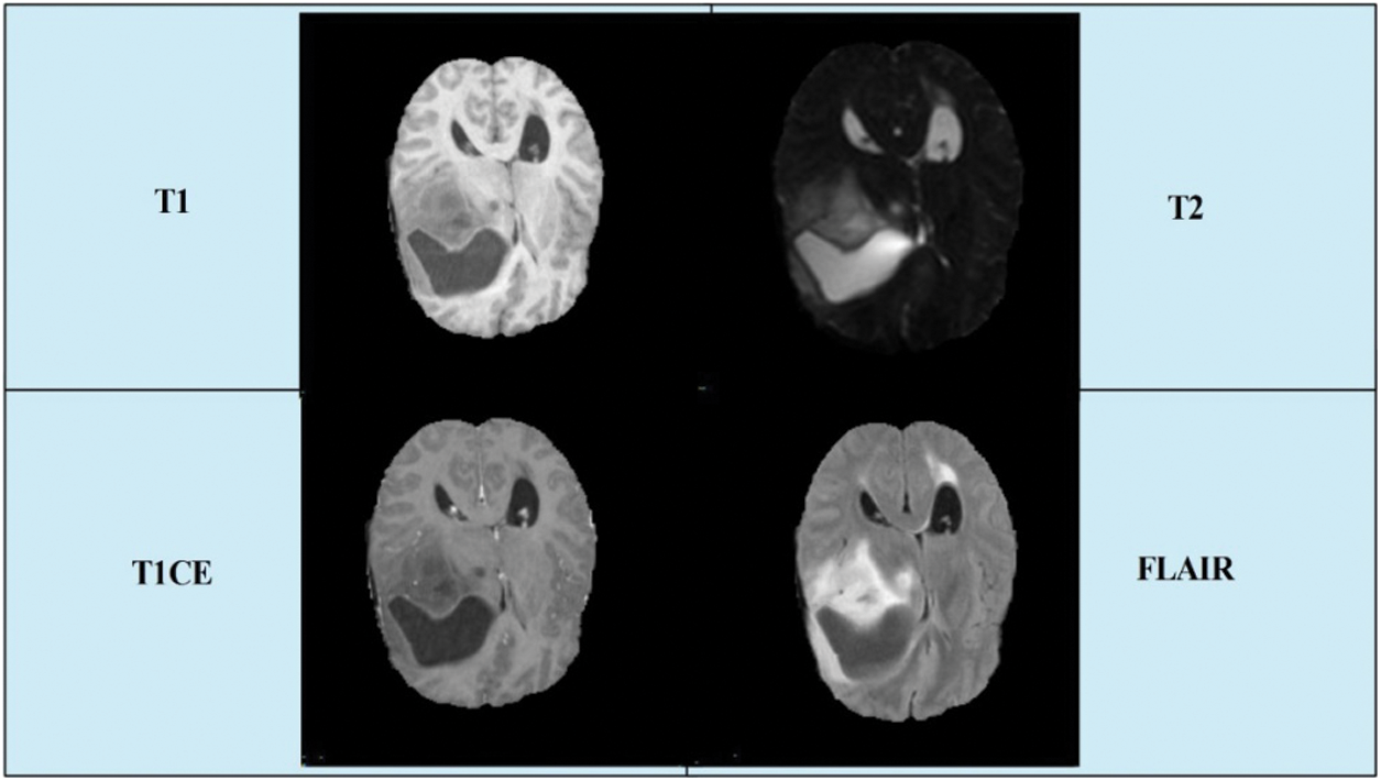
Figure 1: A few sample images collected from BRATS2019 dataset

In addition to being time-consuming, manual brain tumor delineation is difficult and depends on the individual operator [8]. Therefore, proposing automated computerized techniques with minimal human involvement is crucial. Computer vision researchers have introduced many techniques using image processing and machine learning [9,10]. In image processing, they focused on image contrast enhancement and tumor segmentation [11,12], whereas in the machine learning step, they focused on the classification of brain tumors into relevant categories [13]. Contrast enhancement is the most important step in any computerized method developed for medical imaging [14,15]. Based on this step, obtaining the maximum accuracy of the next step is easy [16]. Researchers of computer vision divide computerized techniques into classical approaches [17] and deep learning-based approaches [18]. In the classical approach, four steps are followed for the final classification: enhancement of tumor, tumor segmentation, feature extraction using handcrafted techniques such as texture features, shape features, point features, and Gabor features [19]. Subsequently, these features are fused and classified using supervised learning algorithms [20]. In deep learning techniques, features are extracted from raw images without employing a segmentation step. A simple deep learning model comprises many layers such as convolutional layer, ReLu layer, batch normalization layer, fully connected layer, and softmax. Many deep learning-based techniques have been introduced in the literature, and few of them are discussed here.

Huang et al. [21] presented an automated technique for the detection of brain tumor regions. The proposed method comprises three stages. In the first stage, segmentation is applied. Then, the energy functions were modeled and the energy function was optimized. T1 and FLAIR MRI images were used for the experimental process. They also performed a conditional random field-based framework to merge the information of T1 and FLAIR in the probabilistic region. Islam et al. [22] introduced a new framework based on multi-fractal highlighted and upgraded Adaboost grouping for cerebrum tumor identification. They extracted texture features that were classified using the AdaBoost classifier. The experimental process was conducted using data from 14 patients and achieved better accuracy. Rehman et al. [2] presented a 3D brain tumor detection and classification framework by using deep learning. In this framework, the tumor regions are extracted using a convolutional neural network (CNN) and later utilized for the training of a model. The features of the trained model are extracted from the feature layers and further refined using a correlation-based approach. BraTs datasets were used for the experimental process, and improved accuracy was achieved. Rashid et al. [23] introduced a deep learning-based method for brain tumor classification. They performed a hybrid contrast stretching approach at the initial step and subsequently modified two pre-trained models—VGG16 and VGG19—and subsequently extracted features. They also implemented a correntropy and joint-learning approach for best feature selection. Finally, they implemented a fusion approach. The experimental process was conducted on a BraTs series and achieved improved accuracy.

These techniques still face several challenges, such as i) the contrast of the original MRI images is not suitable for extracting the tumor region. The main problem is the extraction of four diverse MRI slices-which are “T1,” “T1CE,” “T2,” and “Flair.” However, these slices include a shallow contrast that affects the detection problem; ii) the size of the tumor region is not consistent, and it changes for each patient. Therefore, there is a massive chance of error rate for tumor detection; iii) in the feature extraction phase, the key problem is the extraction of irrelevant features, and iv) high similarity among tumor types. In this study, we proposed a new fully automated framework for brain tumor classification using an ensemble of optimal deep learning feature selection. Our significant contributions are as follows.

•   Modified ResNet50 and DenseNet201 were based on the output of the dense layer. The dense layers of both models are updated according to the number of brain tumor classes (i.e., four classes). Subsequently, both models were trained using transfer learning and saved modified models, which were later utilized for feature extraction.

•   An enhanced ant colony optimization algorithm was proposed for the best feature selection. Features were selected from the originally extracted features.

•   A new activation function based on entropy and a normal distribution is proposed. The features passed from this function were selected as the best features and evaluated using the fitness function Fine KNN.

The proposed methodology of multimodal brain tumor classification is presented in Section 2 and includes information on deep learning models, feature selection using meta-heuristic techniques, and final classification. The results are discussed in Section 3. Finally, the conclusions of this study are presented in Section 4.

2  Proposed Methodology

For multimodal brain tumor classification, we herein propose a new enhanced deep learning framework. The first preprocessing step is performed in the proposed framework and then two pre-trained deep learning models, ResNet50 and DenseNet201. Both models were fine-tuned and trained using transfer learning. Subsequently, the features were extracted from the feature layers. The extracted features were optimized using the enhanced ant colony optimization (EACO) algorithm. The selected features of each network are aggregated using a serial-based approach and finally classified using multi-class SVM, where the cubic method is used. A flow diagram of the proposed method is illustrated in Fig. 2.

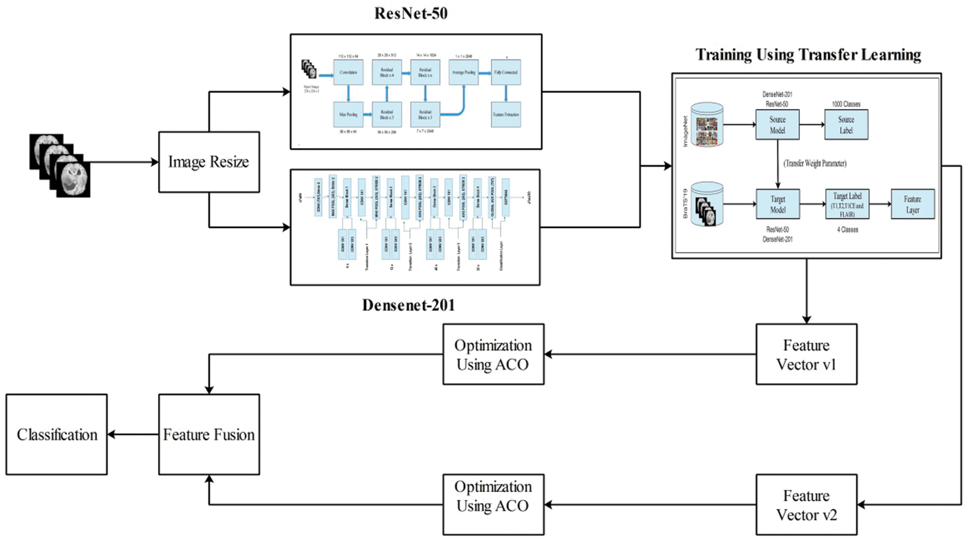
Figure 2: Proposed flow diagram of multimodal brain tumor classification

2.1 Dataset Normalization

In this study, we utilized the BraTs 2019 brain dataset that includes both high-grade glioma (HGG) and low-grade glioma (LGG). The images in this dataset are in MRI format, and each for each patient, four types of scans were generated: T1, T1CE, T2, and Flair. A few sample images are shown in Fig. 1. This dataset consisted of 259 cases of HGG and 76 cases of LGG. All images were manually annotated by clinicians and certified radiologists [24]. In the normalization step, we normalize this dataset into four folders, which are further divided into training and testing. The details of this normalized dataset are listed in Tab. 1.

2.2 Conventional Neural Network

One of the most important deep neural network types is CNNs. It performs image recognition [25,26], image classification [27], and object detection [23]. CNN requires minimal preprocessing compared to the other classification algorithms. This network takes an image as input and is then classified into certain categories. For training and testing, the images are passed through several layers of kernel size and filters. These layers are convolutional layer, pooling, ReLu, fully connected, and softmax. In the convolutional layer, image pixels are transformed into features through a convolutional filter, whereas these features are classified in the softmax layer with probalistic values between 0 and 1.

2.3 Modified ResNet50 Features

ResNet has a better performance; throughout the network, it creates a more direct path for propagating information. In ResNet, backpropagation does not experience a disappearing gradient issue. By avoiding the layers, shortcut networks allowed links that were not beneficial through training. Mathematically, the output T(i) was formulated as follows:

T(i)=R(i)−i (1)

R(i)=T(i)−i (2)

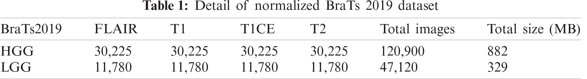
In this study, we utilized the ResNet-50 pre-trained model. This network comprises 64 kernels with a 7×7 convolution layer, a stride 2 by 3×3 max pooling layer, 7×7 avg pooling layer by stride 7, and 16 residual building blocks, and at the end, a fully connected layer. This network has over 23 million trainable parameters. The architecture of ResNet101 is illustrated in Fig. 3.

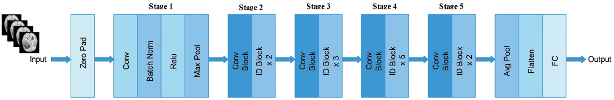
Figure 3: Architecture of ResNet-50 pre-trained deep learning model

Subsequently, we modified this model and removed the last fully connected layer. Originally, this layer comprised 1000 object classes; however, we needed to modify it according to the selected BraTs dataset that only includes four classes. Therefore, we added a new fully connected layer that included only four layers and trained using deep transfer learning. The transfer learning details are provided in the next section. After training through transfer learning (TL), a modified model was obtained. We utilized the modified model and extracted features from the global average pool layer. In this layer, the dimension of the extracted features is N×2048. The modified model is shown in Fig. 4.

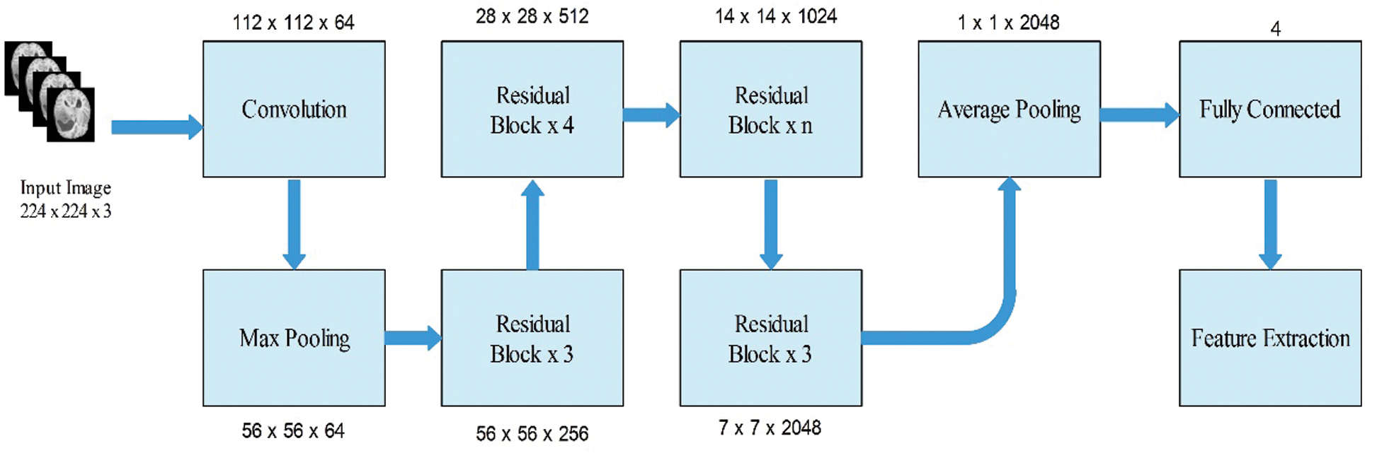
Figure 4: Modified ResNet50 model for brain tumor classification

2.4 Modified DenseNet201 Features

This network comprised 201 deep layers. This network was originally trained on 1000 object classes. In the other deep networks, layers are gradually connected to each other, thereby making the system complex and harder. Recently, the ResNet model provided the concept of skipping layers. Subsequently, the DenseNet network further revised this approach, and sequential concatenation was performed instead of summation of the output features of the previous layers [28]. Mathematically, this is defined as follows:

Z1=Hl ([z0, z1,…,zl−1]) (3)

Here, Hl is a nonlinear transformation, l represents the layer index, and zl represents the features of the lth layer. For down testing purposes, thick squares are created in the organization design that are then isolated by the layers called change layers, which comprise batch normalization, are to be trailed by a 1×1 convolution layer, followed by a 2×2 avg pooling layer. The original architecture of DenseNet201 is shown in Fig. 5.

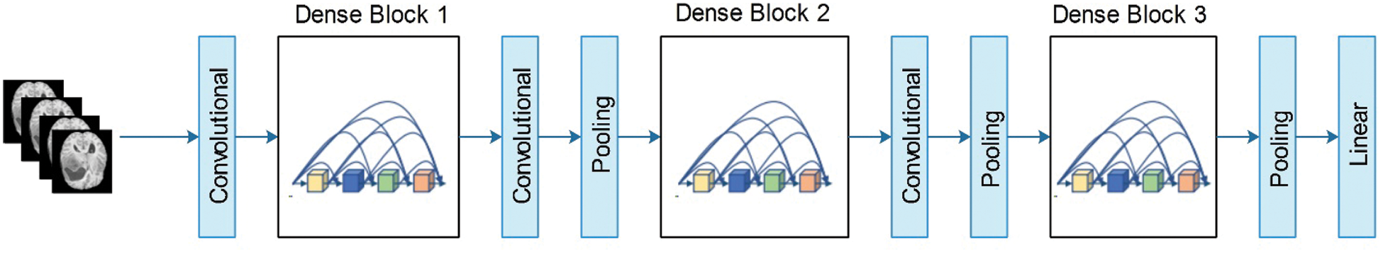
Figure 5: Layered architecture of DenseNet201

In this figure, the pooling blocks utilized in the Densent-201 architecture are shown to reduce the feature map sizes. Each layer in DenseNet consumes direct access to the original contribution image and gradients from the loss function. Thus, the computational rate was significantly reduced. In this study, we modified DenseNet201 for multimodal brain tumor classification. The modified architecture is illustrated in Fig. 6. The fully connected (FC) layer, which originally comprises 1000 object classes, is removed, and a new FC layer that includes only four classes is added. Subsequently, the modified model was trained using TL. In the training process, the number of epochs was 100, the learning rate was 0.00001, and the method was stochastic gradient descent. The mini-batch size was observed to be 64. The newly trained model was saved and later utilized for feature extraction. The features are extracted from the global average pooling layer, which was later utilized for classification purposes.

Figure 6: Modified Densnet-201 architecture

2.5 Transfer Learning and Features Extraction

In deep learning, TL is a process of reusing a model for a target task [29]. The main purpose of TL is to train a pre-trained model instead of training a model from scratch. In this process, source models are considered along with the source data and source labels. Then, we transfer the knowledge to the modified model and train for the new task. In the training process, a few parameters are required, such as stochastic gradient descent, a mini-batch size of 64, a learning rate of 0.00001, and epochs of 100. After training the modified models, the new models were saved for the target task. Mathematically, the TL process is defined as follows:

Qz={(n1z, m1z),…,(niz, miz),…,(nyp, myp)} (4)

The learning task is defined as follows:

lk, lz{(nwz, mwz)∈R} (5)

The target domain is defined as follows:

Ts={(n1s,m1s),…,(nis,mis),…,(nws,mws)} (6)

The learning task with target domain is defined as follows:

lt=(nys, mys)∈R, (w, y) (7)

where y<<w and m1Q, m1s are the training data labels. This process is illustrated in Fig. 7. In this figure, the source models ResNet50 and DenseNet201 have 1000 object classes. In the TL, the knowledge is transferred, and the modified models are trained. After training both models, features are extracted from the last layers (global average pool) and utilized for the next process. From both layers, the sizes of the extracted feature vectors are N×2048 and N×2048.

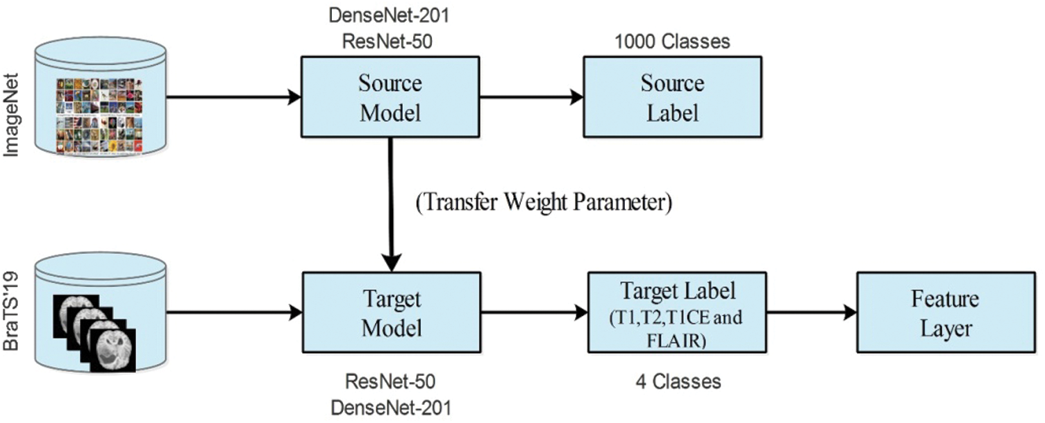
Figure 7: Transfer learning process for brain tumor classification

2.6 Features Optimization Using EACO

The ability to correct classification within a minimum time is based on the selection of features [30]. Most extracted features are not relevant to the classification phase and have an impact on accuracy. Feature selection is the process of selecting the best subset from the original features. Many techniques have been implemented in the literature, such as genetic algorithm-based selection, PSO-based selection, Grasshopper-based selection, and entropy-based selection [31]. The most relevant features are selected through feature selection techniques, and irrelevant features are removed based on the defined criteria. We proposed an EACO algorithm for the best feature selection herein. In this algorithm, ants are initially defined, and the probability for decision is then computed. Subsequently, the rule of transition is applied, and the pheromones are updated. Subsequently, features are passed in the new activation function, which is based on entropy and normal distribution. The features passed from this function are selected as the best features and evaluated using the fitness function fine KNN. The details of each step are defined as follows.

Originally, ACO was inspired by the behavior of ants. The behaviors of ants include checking the temperature of the nest, forming the bridges, going to raid the specific area for food, building and protecting the nest, sorting the brood and the items of food, carrying the large items cooperate with each other, colony to emigrate, and obtaining the shortest route from nest to food source.

Starting Ant Optimization-The no of ant computed as:

AN=l×x (8)

where l represents the feature vector, x represents the width of the feature vector, and AN denotes the total number of ants used for the random placement in the feature vector based on each feature value, where one feature contains one ant.

Decision Based on Probability-The probability of traveling of ant n is pij through feature (e,f) to feature (g,h). The probability can be formulated as follows:

pef=(pef)(pef)a∑f∈Q(pef)a(xef)auef(Δ) (9)

when e, f∈Ω. Here, every value of the feature location is given as e, f∈Ω. pef denotes the quantity of pheromones, xef represents visibility, and its value is explained with the help of the following formulation:

xef=Hef (10)

Based on pef, the ∆ plus finds the quality of fluctuation in direction on every step. It can be defined as follows:

Δ=0, π/4, π/2, 3π/4, π (11)

Rules of Transition-Mathematically, this rule is defined as follows:

S={arg⁡{maxj∈Q[(ρij)a(xij)buij(Δ)]}}, (12)

where q<qo, i and j represents the feature locations and these features are traveling to a location (k,l). If q>q0, then the next feature that should be visited is chosen by the ants.

Pheromone Update-In this step, the ants are to be shifted from pixel ij to update the feature location (k, l). Based on it, the path of the pheromone is to obtain after every of the iteration and mathematically it is define as follows:

ρij=(1−η).ρij+η.Δρij (13)

Δρij=xij (14)

Here, η(0<η<1) shows the ratio of an evaporation of a pheromones. A new values of pheromones is obtain after every iterations and mathematically, it is defined in Eq. (15) as follow:

ρij=(1−θ).ρij+θ.ρ0 (15)

Here, θ(0<θ<1) shows promotions of evaporated pheromones. New values of pheromones and ρo represent the start values of the pheromones. These steps are applied for all features, and in the outputs, we obtain a new robust feature vector.

Feature activation function: A new activation function is proposed to modify the output of the ACO algorithm. This function is based on normal distribution and entropy values. Both values were multiplied and compared with the original ACO-based selected features. Features with values greater than the multiplication value (normal distribution and entropy) were selected for the final classification. Mathematically, this process is defined as follows:

g(f)=1σ2πe−12(fi−μσ)2 (16)

H(f)=∑fP(f).log⁡(1p(f)) (17)

Activation={Sel(fi)for fi≥g(f)∗H(f)discard,Elsewhere (18)

The final selected features were represented by Sel(fi) and classified using machine learning algorithms. This process was applied to both modified deep learning models for the best feature selection. Finally, both selected vectors are fused using a serial-based approach that followed the final classification.

3  Experimental Results and Discussion

The BraTs2019 dataset was used for the experiments herein. The setup was carried out at a 70:30 ratio and was used to evaluate the system. Ten-fold cross-validation was applied to the experimental results. Cross-validation is a re-sampling process used to evaluate the machine learning models on a limited data sample. Various classifiers such as linear discriminant, linear SVM, quadratic SVM, cubic SVM, medium Gaussian SVM, fine KNN, subspace KNN, weighted KNN, subspace discriminant, and medium KNN are used. Each classifier is evaluated based on importance measures, including the recall rate, precision rate, accuracy, and computational time. MATLAB2020b was used for the simulation, where the system used had a Core i7 CPU, 16-GB RAM, and 8-GB graphics card. Furthermore, the deep learning toolbox Matconvnet was applied for deep feature extraction.

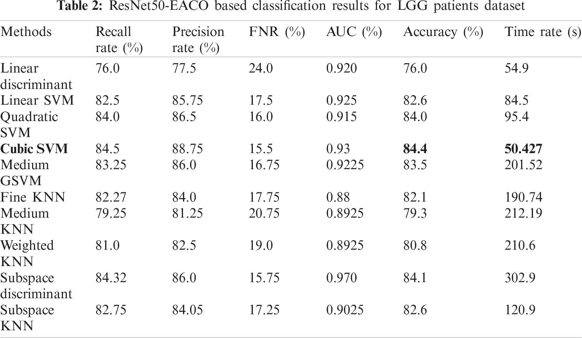
The results of the proposed method are presented herein. The results were computed for both the HGG and LGG patient data. Initially, the results are presented for modified ResNet50-EACO for both LGG and HGG. The results are presented in Tabs. 2 and 3. Tab. 2 presents the results of ResNet50-EACO for the LGG data. In this table, the accuracy of the cubic SVM is 84.4% with a recall rate of 84.5%, a precision rate of 88.75%, and the time taken is 50.427 s. The second-best accuracy is 84.1%, achieved by subspace discriminant, along with 84.325% recall rate, 86% precision rate, and 0.98 area under curve. The remaining classifiers also exhibited better performance. The computational time of this approach was significantly minimized (50%) compared to all features of the modified ResNet50. In addition, the accuracy of the proposed approach increased by 7%–8%. The accuracy of the cubic SVM can be further confirmed by Fig. 8 in the form of a confusion matrix.

Figure 8: Confusion matrix of Cubic SVM using ResNet50-EACO on LGG dataset

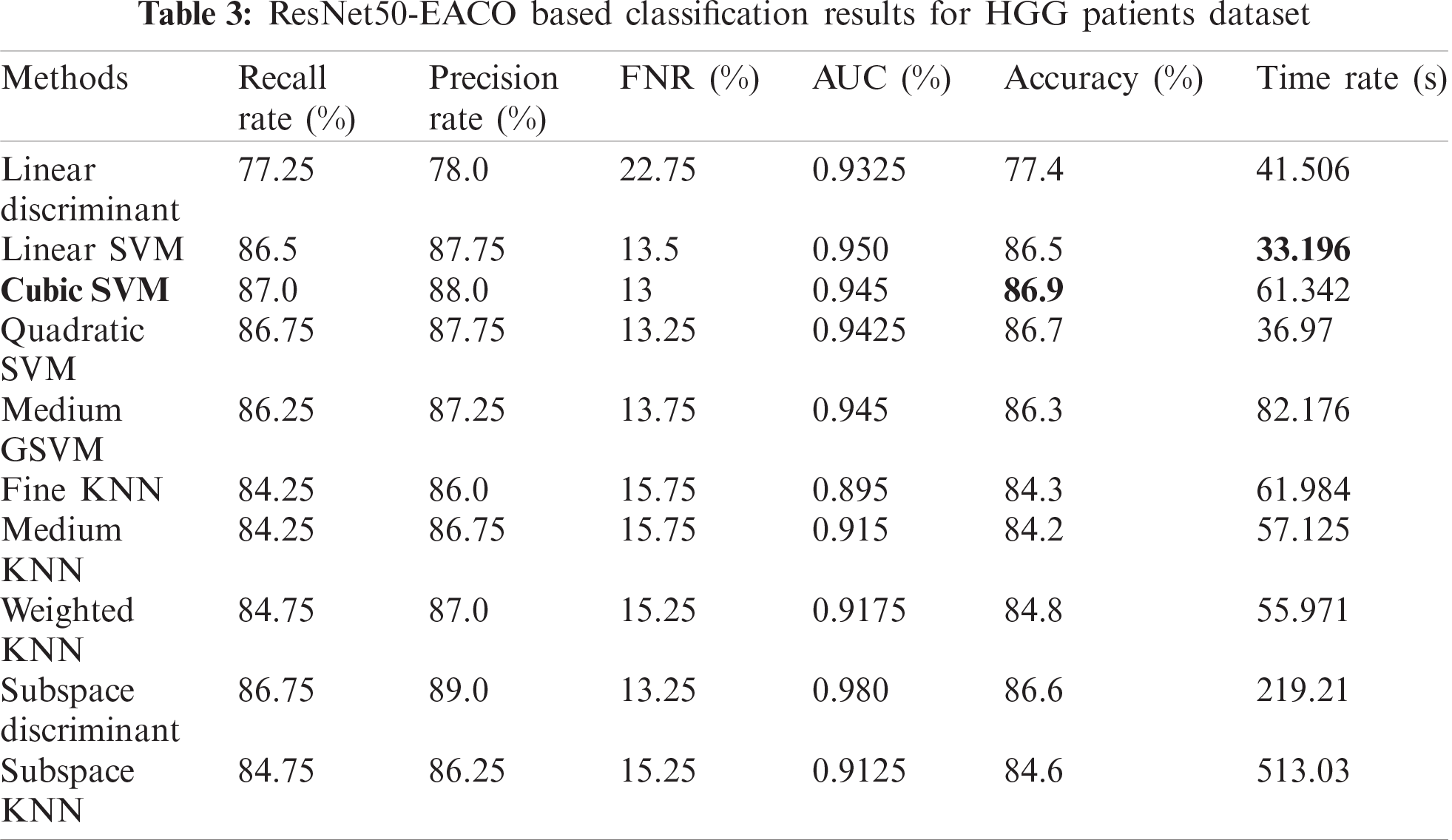
Tab. 3 presents the results of the HGG data for the ResNet50-EACO approach. The cubic SVM achieved the best accuracy of 86.5%, whereas the rest of the calculated measures had recall rates of 86.5% and 87.75% of the precision rate, and the area under the curve was 0.95. This performance can be confirmed by the confusion matrix shown in Fig. 9. The minimum computational time for this experiment was 33.196 s. Similar to the LGG data, the performance in terms of accuracy was improved, and the computational time was minimized by almost 45%.

Figure 9: Confusion matrix of Cubic SVM using ResNet50-EACO on HGG dataset

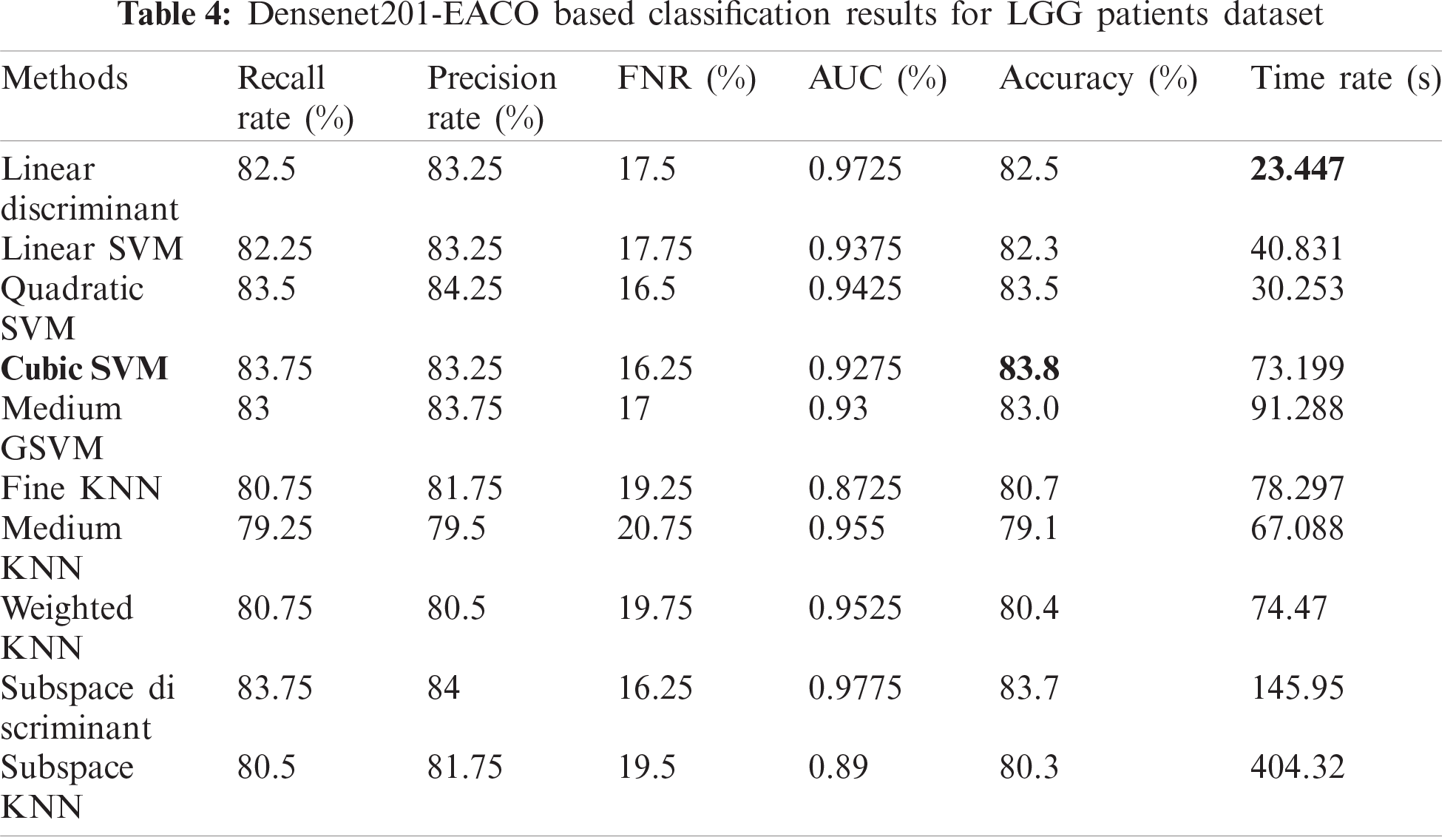
Tab. 4 presents the results of Densenet-EACO for the LGG data. In this table, the accuracy of the cubic SVM is 83.8% with a recall rate of 83.75%, a precision rate of 83.25%, and the time taken by it is 73.199 (s). The accuracy of the cubic SVM can be further confirmed by Fig. 10 in the form of a confusion matrix. The second-best accuracy was 83.5%, achieved by quadratic SVM along with 83.5% recall rate, 84.25% precision rate, and 0.9425 area under curve. The remaining classifiers also exhibited better performance. The computational time of this approach is significantly minimized (40%) compared to all the features of the modified Densenet201. In addition, the accuracy of the proposed approach is increased to 8%.

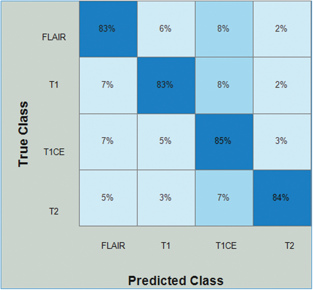
Figure 10: Confusion matrix of Cubic SVM using Densenet201-EACO on LGG dataset

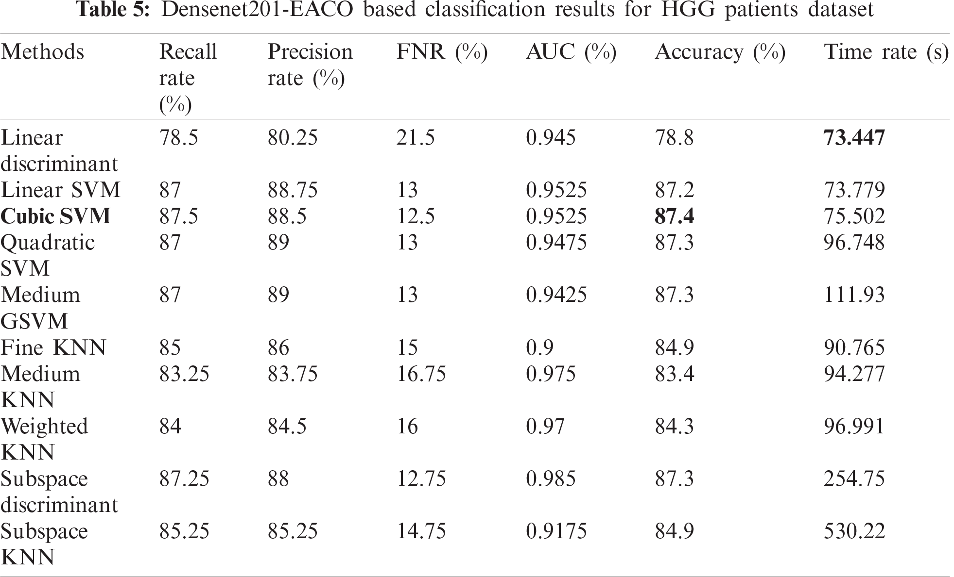
Tab. 5 presents the results of the HGG data for the Densenet-EACO approach. The cubic SVM achieved the best accuracy of 87.4%, where the rest of the calculated measures had recall rates of 87.5% and 88.5% of the precision rate, and the area under the curve was 0.9525. This performance can be confirmed by the confusion matrix shown in Fig. 11. The minimum computational time of this experiment was 73.447 s for the linear discriminant classifier. Using this new approach, the accuracy is improved, and the computational time is significantly minimized.

Figure 11: Confusion matrix of Cubic SVM using Densenet201-EACO on HGG dataset

Finally, we fused the feature information of Densenet201-EACO and ResNet50-EACO for both types of data (LGG and HGG). After the fusion process, the accuracy of HGG data reaches 87.8% (cubic SVM), where the other measures are as follows: recall rate is 87%, precision rate is 88.5%, and FNR is 13%. For LGG, the accuracy increased to 84.6% (cubic SVM). The fusion-based accuracy was improved and reliable for better classification. This is illustrated in Fig. 12. The main strength of the proposed framework is the selection of the best features using EACO. Using this approach, obtaining the best features and achieving improved accuracy is easy.

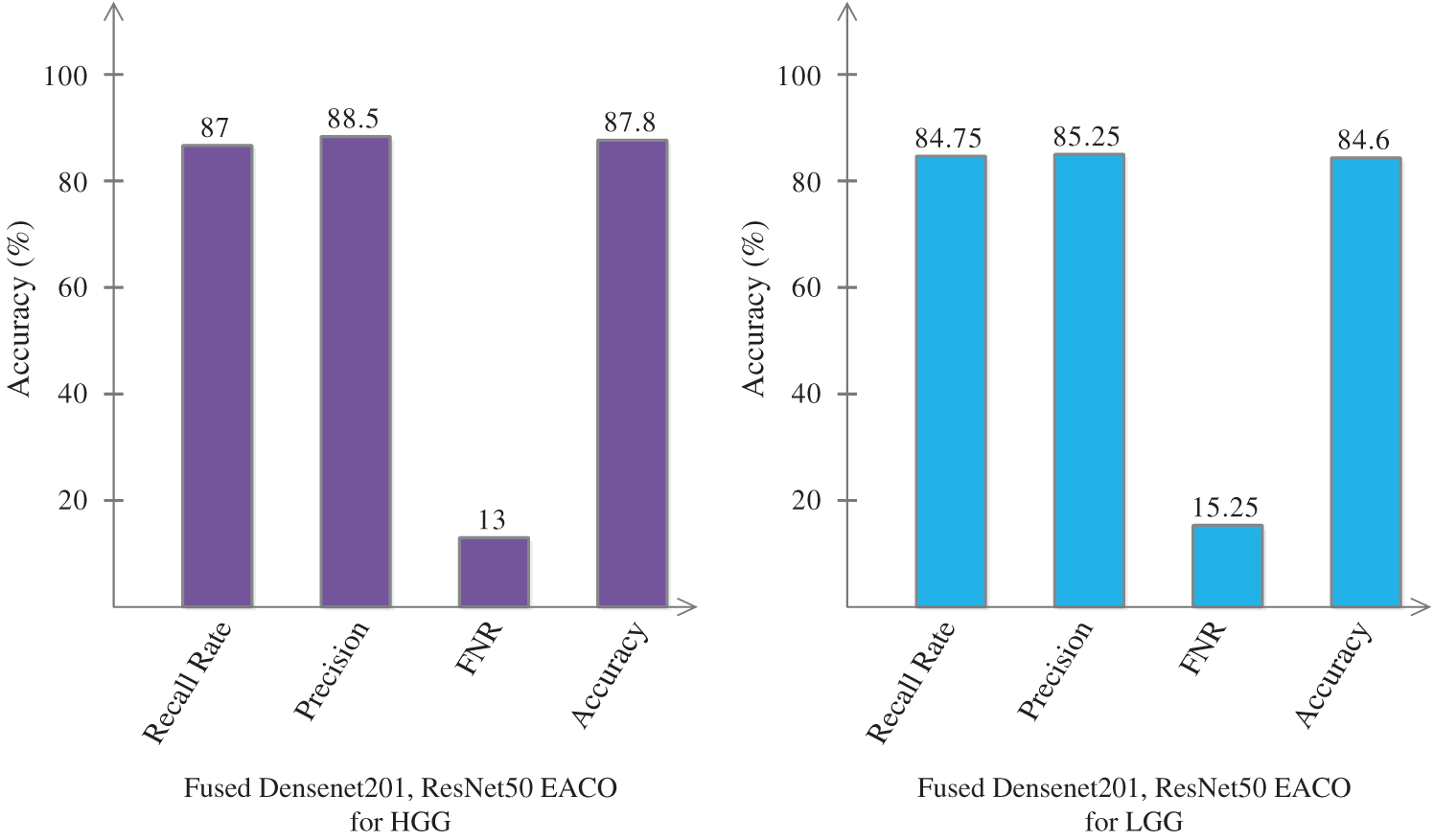
Figure 12: Proposed classification results of cubic SVM after the fusion of optimal features

4  Conclusion

An ensemble framework was proposed in this study for multimodal brain tumor classification. The proposed framework is based on the fusion of optimal deep learning features. A series of steps are employed in this framework: i) collection of database and normalization of the dataset; ii) selection of two pre-trained models and modification of both models; iii) training of both modified models for brain tumor classification using TL; iv) proposing an EACO algorithm for optimal feature selection; and v) fusion of both optimal features for the final classification. The experimental process was conducted on the BraTs2019 dataset, and we achieved exceptional accuracy. Based on the results of the proposed framework, we can conclude that the EACO-based feature selection algorithm showed improved accuracy (approximately 8%) and minimized computational time. Furthermore, this process removes the redundant features. The improvement in the ACO in the form of an activation function also increased the reduction of redundant features. The key limitation of this framework is the fusion of the optimal features. After the fusion process, the accuracy of the proposed method increases, but the testing time also increases. We will consider this issue in future studies and develop a single-step feature selection approach without feature fusion.

Funding Statement: This study was supported by the grants of the Korea Health Technology R&D Project through the Korea Health Industry Development Institute (KHIDI), funded by the Ministry of Health & Welfare (HI18C1216), the grant of the National Research Foundation of Korea (NRF-2020R1I1A1A01074256), and the Soonchunhyang University Research Fund.

Conflicts of Interest: The authors declare that they have no conflicts of interest to report regarding the present study.

This work is licensed under a Creative Commons Attribution 4.0 International License, which permits unrestricted use, distribution, and reproduction in any medium, provided the original work is properly cited.