DOI:10.32604/cmc.2021.018390
| Computers, Materials & Continua DOI:10.32604/cmc.2021.018390 | |
| Article |
An Optimized Design of Antenna Arrays for the Smart Antenna Systems
1Department of Computer Science, King Khalid University, Muhayel Aseer, Kingdom of Saudi Arabia
2Faculty of Computer and IT, Sana'a University, Sana'a, Yemen
3Department of Electrical Engineering – Communication Engineering, Sana'a University, Yemen
4School of Computing, Faculty of Engineering, Universiti Teknologi Malaysia, Malaysia
5Department of Electronics and Communication Engineering, Faculty of Engineering, University of Aden, Yemen
6Department of Information Systems, King Khalid University, Muhayel Aseer, Kingdom of Saudi Arabia
7Department of Computer Science, College of Computers and Information Technology, University of Bisha, KSA
* Corresponding Author: Fahd N. Al-Wesabi. Email: fwesabi@gmail.com
Received: 07 March 2021; Accepted: 17 April 2021
Abstract: In recent years, there has been an increasing demand to improve cellular communication services in several aspects. The aspect that received the most attention is improving the quality of coverage through using smart antennas which consist of array antennas. this paper investigates the main characteristics and design of the three types of array antennas of the base station for better coverage through simulation (MATLAB) which provides field and strength patterns measured in polar and rectangular coordinates for a variety of conditions including broadsides, ordinary End-fire, and increasing directivity End-fire which is typically used in smart antennas. The method of analysis was applied to twenty experiments of process design to each antenna type separately, so sixty results were obtained from the radiation pattern indicating the parameters for each radiation pattern. Moreover, nineteen design experiments were described in this section. It is hoped that the results obtained from this study will help engineers solve coverage problems as well as improve the quality of cellular communication networks.
Keywords: Smart antenna; antenna arrays; patterns construction; coverage
The concept of smart antennas has existed for many years, and it has received a wide attention [1]. Cellular networks require coverage, and coverage depends on the type of antenna and the antenna radiation pattern [2]. The cellular base station antenna in the cell sector uses a reflective angle antenna that radiates into the cell at a limited angle according to the area's coverage requirements. The radiation itself depends on several parameters [3,4].
Single-component antennas have relatively broad radiation patterns because the gain and direction are low. When the antenna is electric, the size increases by expanding the radiation dimensions to obtain more excellent directivity, but still, all these methods lead to a decrease in the antenna's efficiency. The radiation model contains several side lobes and when building a group of radioactive elements that include appropriate electric fields and the correct geometry, we get an increase in the antenna's electrical volume. These antennas are called matrix antennas. The matrix radiation patterns are based on relative positions (single radiators, field currents, individual radiator currents or fields, and individual radiators) [5–8].
Hence, the representation of the matrix elements gives a radiation pattern characterized by direction and gains different from that of a single antenna element.
Coverage quality depends on several requirements, such as channel capacity, best signal quality, lowest transmission capacity, highest data rate, and new added value for existing mobile wireless communication services in telecommunication networks, to meet these requirements. This is considered one of the technological challenges that face service providers. It was introduced in the form of “smart antennas” or “adaptive array antennas,” which has enhanced coverage and brought many benefits to cellular carriers [9–11].
Several types of antennas have been used in various smart communication and detection systems. In [12], an antenna system has been proposed and controlled by p-i-n diodes with the ability of radiation pattern changing between six states in the azimuth plane. In [13], a smart antenna with beam switching capability has been proposed that can realize beam switching between 0, 90, 180, and 270° by using diodes. In [14], a two-dimensional scanning smart antenna has been developed for cognitive radio. In [15], a smart antenna array has been designed by using various types and nonuniformly distributed elements to process multiple signals at multiple frequencies simultaneously. In [16], a shape changeable parabolic smart antenna system is presented to transmit a signal with a predefined gain to desired positions by controlling the shape of the antenna using a shape-memory alloy. In [17], a smart antenna system has been proposed with interfering moderation capability that is realized by generating radiation nulls in the interferer direction. In [18], a novel reconfigurable adaptive linear array has been designed for providing the optimal radiation direction in which the spatial correlation coefficient is minimal, and in [19], the antenna is further formed to minimize the spatial correlation coefficient. In. [20], a beam-steering reconfigurable antenna system has been developed to searching for the maximum receiving signal energy. In [21], a beam tracking scheme has been proposed in the downlink of 5G cellular radio access that can choose candidate beams based on mobility-reference signals.
Although all of these antennas have been used in wide applications of smart mobile communication systems, the external control systems must be used, and more of those antennas do not have the capability of sensing and setting their features to fit with environmental information. However, these antennas presented in the literature [12–21] cannot be seen as smart antennas.
This research aims to study and analyze three types of antenna array (broadside array, ordinary End- fire array, and increased directivity end–fire array) and select the best type for ideal coverage. The antenna array design relies on two main parameters (distances between sources in radians, and the number of sources, to plot the radial field and energy pattern. The shape and energy of the radiation pattern depend on the values of the main parameters (half-power beamwidth (HPBW), the phase between sources, gain in (dB), gain in (dBi), and first beamwidth blank (BWFN)).
Therefore, the research's importance is completed by designing a simulation that includes designing three types of antenna array and showing the radiation pattern, energy, and the values of its main parameters. Under which the best kind is chosen to meet the coverage quality of cellular communication cells.
The remainder of the article is structured. In Section 2, we explain the proposed system model. In Section 3, we present the theoretical analysis and formulation. Software development and simulation are provided in Section 4. Results analysis and discussion are provided in Section 5. Discussion is provided in Section 6, and finally, we conclude the article in Section 7.
Suppose a system model has three core types of antenna arrays which are broadside array, ordinary end-fire array, and increased directivity end-fire array. Input and output simulation has been performed for each of those antenna arrays to get better coverage. Input simulation covers main three issues which are the select type of antennas array (T), spaces between the sources (D), and the number of sources (N). However, the output simulation covers main seven issues which are field patterns, power patterns, half-power beamwidth (HPBW), beamwidth first null (BWFN), gain (G) in (dBi), gain (G) in (dB), and phase between sources (δ) as illustrated in Fig. 1.
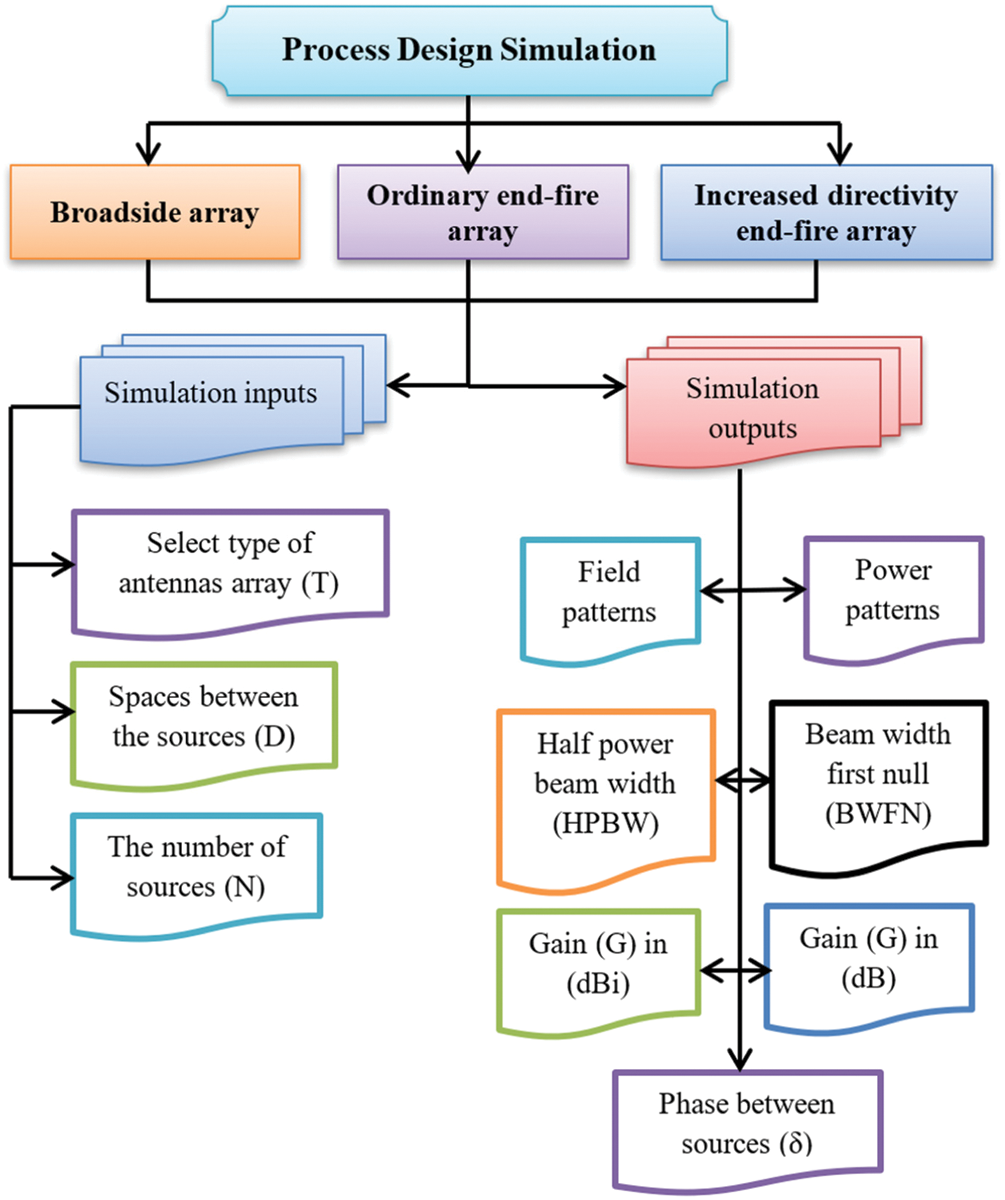
Figure 1: The main components of the proposed system model
3 Theoretical Analysis and Formulation
3.1 Linear Arrays of Isotropic Point Sources of Equal Amplitude and Spacing
Consider now the case of the sources, the characteristics of the equivalence point of capacitance and spacing in a linear array and the whole field spacing between sources is λ/2. These arrays have no minor lobes. E at a considerable distance in the direction is ϕ as given by Eq. (1).
where:
ψ—The total phase difference of the fields from adjacent sources.
d—The spacing between sources.
n—Is any positive integer.
Fig. 2 represents a unit source so that the breadth of the field of all sources is equal and taken as a unit source and the shape is considered a reference stage. At a distant point in the direction, we found that:
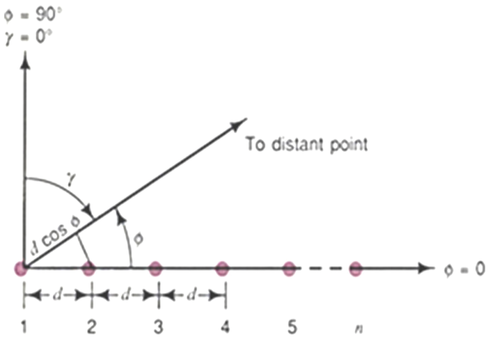
Figure 2: Isotropic point sources are produced from a linear array
— The field from source 2 is advanced in phase concerning to source 1 from ψ.
— The field from source 3 is advanced in phase concerning source 1 by 2 ψ, etc. equal amplitude and spacing in a linear array.
When adding a phasor (vector), we obtain both the amplitude of the total field E and its phase angle ζ as given by Eq. (2) and illustrated in Figs. 3a and 3b.
And from Eq. (3) below.
It may be rewritten as shown in Eq. (4).
From Eq. (5) given below.
where ζ is referred to the field from source 1, the value of ζ is given by Eq. (6).
If the phase refers to the center point of the array, Eq. (5) becomes as shown in Eq. (7).
In this case, the phase pattern is a step function given by Eq. (7). The phase of the field is constant wherever E has a value but changes sign when E goes through zero. When ψ = 0, 5 or 7 am indeterminate so that in this case, E must be obtained as the limit given by Eq. (7) above as ψ approaches zero. Thus, for ψ = 0, we have the Relation that (E = n).
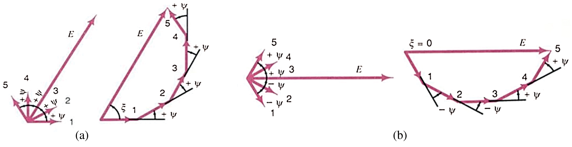
Figure 3: Addition of fields of different phases arriving at a distant point from a linear array of five isotropic sources of equal amplitude with the phase of source 1 for (a) and source 3 for (b)
This is the maximum value that E can attain the normalized value of the whole field for Emax = n is a normalized array pattern as shown in Eq. (8).
For a 5-source array with λ/4 spacing and δ = −90 progressive phasing is as shown in Eq. (9).
We note that this 5-source array would be called an ordinary end-fire array as shown in Eq. (10).
The broadside array (source in phase) is a linear array of an isotropic source of the same amplitude and phase. Therefore δ = 0 and to make ψ = 0 requires that ϕ = (2k+1) (π/2).
Where k = 0.1.2.3…, the field is maximum as shown in Eq. (11).
Fig. 4 shows the radiation pattern of the broadside array of four-point sources and the phase spacing by λ/2, and certainly the point sources here have the same amplitude.
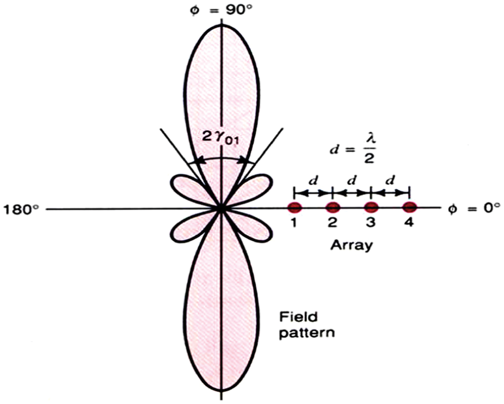
Figure 4: The field pattern of broadside array
The phase angle between adjacent sources is required to make the field a maximum in the direction array (ϕ = 0). An array of this type may be called an end-fire array. For this we substitute the conditions (ψ = 0 and ϕ = 0).
From Fig. 5 above, as we observe, represents the radiation pattern of the usual end-fire array for four isotropic point sources, and the distance between the reference here is λ/2 and δ = −π, which is an example of the bidirectional pattern.
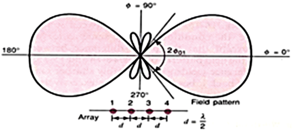
Figure 5: The field pattern of ordinary end-fire array
3.4 End-Fire Array with Increased Directivity
The situation discussed in case 2, namely, for δ = −(2πd/λ), produces a maximum filed at the direction ϕ = 0 but it does not give the maximum directivity. A larger directivity is obtained by increasing the phase change between sources as shown in Eq. (12).
This condition will be referred to as the condition for “increased directivity,” thus for the phase difference of the fields at a considerable distance as shown in Eq. (13).
Any increased directivity end-fire array, with a maximum at ψ = −π/n, has a normalized field pattern given by Eq. (14) of the array pattern (increased directivity).
Fig. 6 shows the radiation pattern of end-fire array four isotropic point sources where equal amplitude spacing is λ/2 and the progressive phase angle δ = −(5π/4).
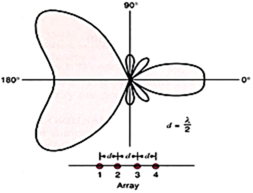
Figure 6: The field pattern of the end-fire array
4 Software Development and Simulation
To evaluate the performance of the proposed system model and select the best antenna array, the self-developed software has been developed using Visual Basic.net programming language and simulated software has been developed using MATLAB environment. This section explains in detail the developed and simulation software.
The simulation has been performed using MATLAB programming language. The simulation aims to study each type of antennas array (broadside array, ordinary end-fire array, and increased directivity end-fire array) and choose the best type for ideal coverage. The simulation depends on two main parameters which are spaces between the sources (D) in radians, and several sources (N) to plot the field and power patterns. These parameters allow the user to enter the values after the selected type of antenna arrays (T).
The simulation of the proposed system model shows the radiation pattern and calculates the main parameters as follows:
• The half-power beamwidth (HPBW).
• The Phase between sources (δ).
• Gain (G) in (dBi).
• Gain (G) in (dB).
• Beamwidth first null (BWFN).
Fig. 7 shows the main window of the developed software.
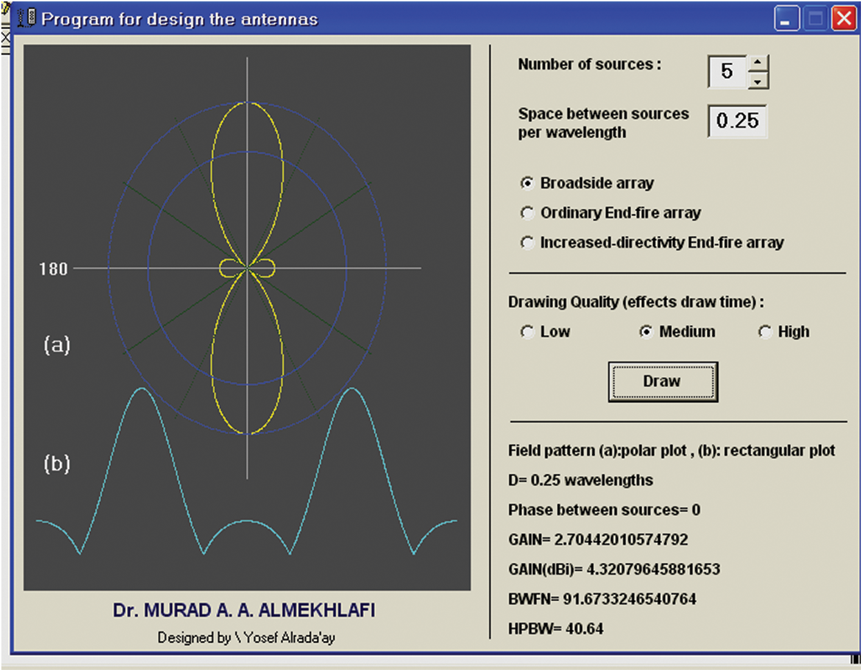
Figure 7: The core parameters of the developed software of the proposed system model
5 Results Analysis and Discussion
In this section, the simulated antennas arrays are critically analysed which are (broadside array, ordinary end-fire array, and increased directivity end-fire array) through two stages. The first stage is space between the sources (D). However, the second stage is a number of sources (N) as shown in Fig. 8 to plot the field and power patterns (pattern construction) with calculates the main parameters (half-power beamwidth (HPBW), the phase between sources (δ), gain (G) in (dBi), gain (G) in (dB), and beam width first null (BWFN).
Fig. 8 shows some examples of the effect of the number of sources (N) and the space between the sources (D) for pattern construction. The method of analysis was to apply twenty experiments of process design to each antenna type separately, so sixty results were obtained from the radiation pattern indicating the parameters for each radiation pattern, and nineteen design experiments were described. The following subsection shows each branch of the mentioned stages.
Figure 8: The effect of a number of sources (N) and the space between the sources (D) for the field and power patterns: (a) (N = 5) and (D = λ/2). (b) (N = 2) and (D = λ)
This subsection explains the simulation using the parameters of space between sources to analyze these effects on the field pattern.
We used the Broadside array type to examine the spacing effect on the pattern field. When the space between sources equals 0.25 λ, the antenna radiates in two directions, and the half-power beamwidth in two approaches is the same as shown in Tab. 1. When space increases up 0.25 λ, the half-power beamwidth decreases and shows a side lobe. When the space increases to λ, the half-power beamwidth for side lobes increased. When space is smaller than 0.25 λ, the radiation pattern approaches from a circular shape. The perfect case for broadside is when space equals 0.25 λ as shown in Tab. 1 and illustrated in Fig. 9.
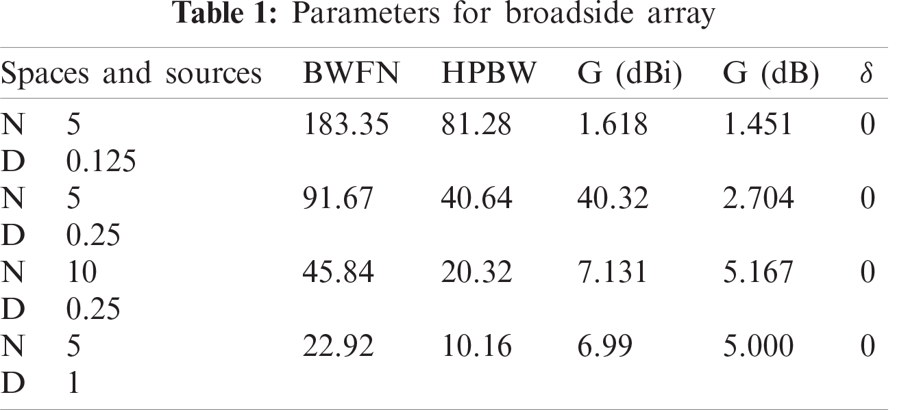
It can be noted From Fig. 9b that the antenna radiated in two directions, front and back. This radiation has the same half-power beamwidth. We found that half-power beamwidth (HPBW) of the pattern has little radiation and the gained coefficient is more extensive, so it is very appropriate to cover limited areas.
Figure 9: The perfect case for broadside with: (a) (N = 5) and (D = 0, 125), (b) (N = 5) and (D = 0, 25), (C) (N = 10) and (D = 0, 25), and (d) (N = 5) and (D = 1)
5.1.2 For Ordinary End-Fire Array
The antenna radiates in two directions, also front and back at the same of broadside array type, but the half-power beamwidth is more extensive. Since the half-power beamwidth is complete, we used this type when the regional coverage is open because the radiation pattern does not meet obstructions. The results show an HPBW, phase between sources (δ), gain (G), and beamwidth first null (BWFN) from the simulation, which can be seen in Tab. 2 and illustrated in Fig. 10.
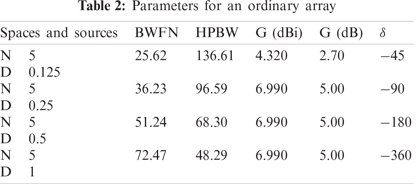
Figure 10: The perfect case for ordinary end–fire array with: (a) (N = 5) and (D = 0.125), (b) (N = 5) and (D = 0.25), (C) (N = 5) and (D = 0.5), and (d) (N = 5) and (D = 1)
5.1.3 For Increased Directivity End–Fire Array
The antenna for increased directivity end-fire radiates in two directions, but the half-power beamwidth is different from one order to another. The radiation pattern has taken a concavities shape, as shown in Tab. 3 and illustrated in Fig. 11.
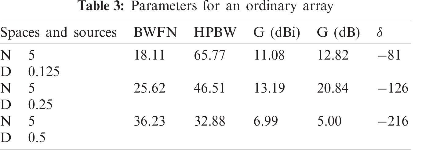
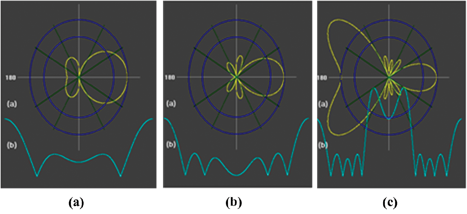
Figure 11: The perfect case for increased directivity end–fire with: (a) (N = 5) and (D = 0.125), (b) (N = 5) and (D = 0. 25), and (C) (N = 5) and (D = 0.5)
Therefore, we used this type when the regional coverage is contained not a desired coverage. It can be concluded that: each antenna has a different radiation pattern, and each type pattern has an application characteristic that depends on the geographical nature of the region, which desired coverage; also it can be mixed between those types in one part according to the object of coverage.
This subsection explains in detail the simulation using the parameters of a number of sources to analyze these effects on the field pattern, and we note that changing the number of sources caused changing in the shape of the radiation pattern.
It can be observed that the changed number of sources caused half-power beamwidth changes. If the number of sources increases, the half-power beamwidth decreases. The radiation pattern takes an asymmetric shape. However, when the value of N up to 10, the radiation pattern takes a non-symmetric shape. The perfect case of this type is at N ring as shown in Tab. 4 and illustrated in Fig. 12.
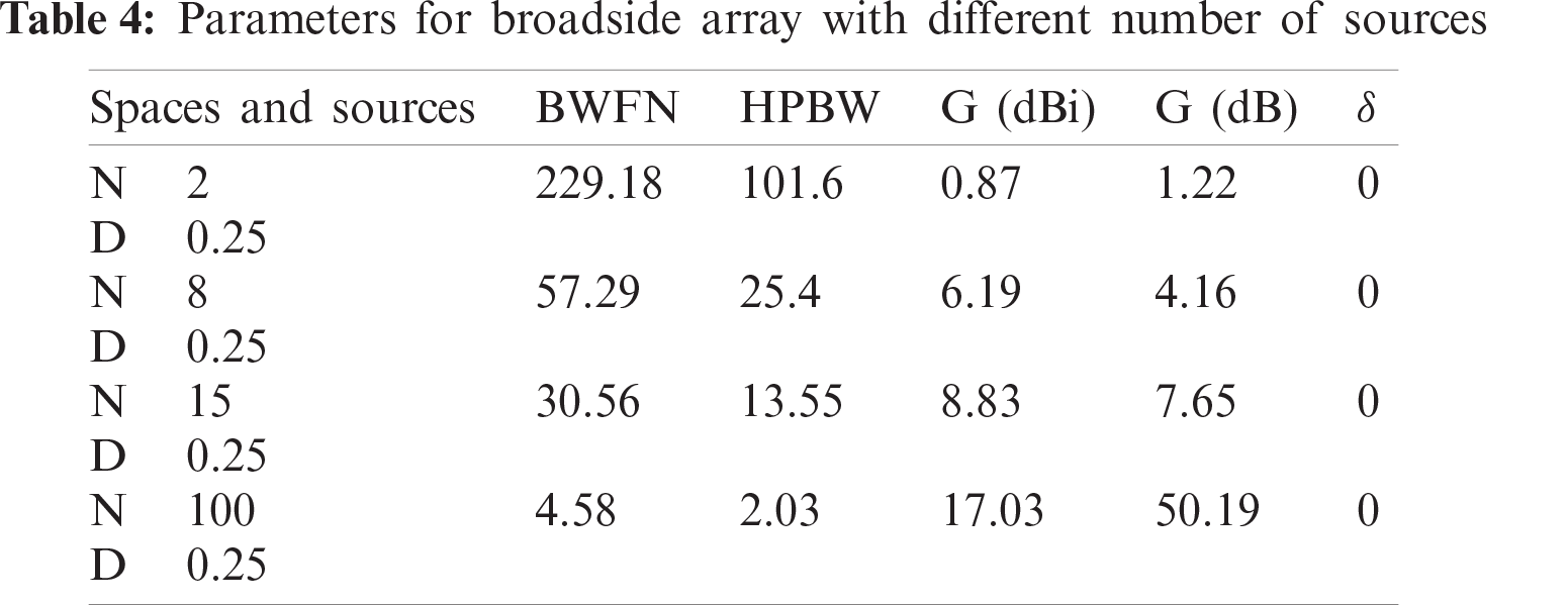
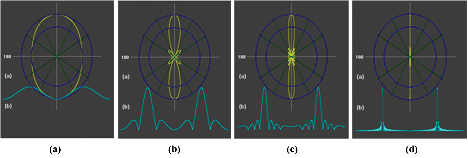
Figure 12: The perfect case for increased directivity end –fire with: (a) (N = 2) and (D = 0.25), (b) (N = 8) and (D = 0.25), (C) (N = 15) and (D = 0.25), and (d) (N = 100) and (D = 0.25)
As observed, the width of the half-power beam for side lobes increases when the space between the arrays begins to rise and approaches the wavelength. The radiation pattern is close to the circular shape when the space between the arrays is smaller than 0.25 λ. When crowded (throttling) areas are to be covered, the Broadside array can help prevent a large number of radiation reflections from the barriers.
5.2.2 For Ordinary End-Fire Array
The same case appears, where, when N increases, the half-power beamwidth decreased, and the radiation pattern is taking a symmetric shape. The perfect case of this type is at N rung, as shown in Tab. 5 and illustrated in Fig. 13.
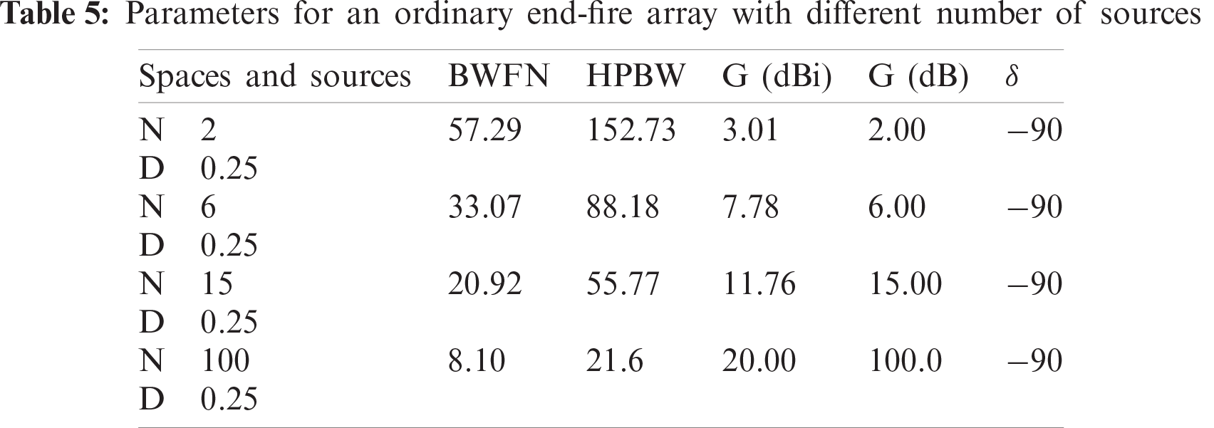
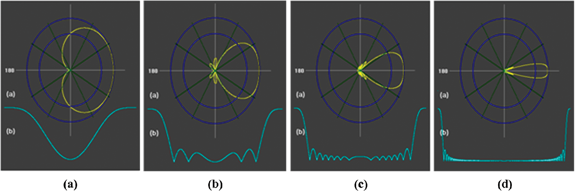
Figure 13: The perfect case for ordinary end-fire array with: (a) (N = 2) and (D = 0, 25), (b) (N = 6) and (D = 0.25), (C) (N = 15) and (D = 0.25), and (d) (N = 100) and (D = 0.25)
From Fig. 13, we noted that directionality and gain can be improved. Still, the presence of side lobes may cause some interference problems, depending on the region in which this radiation pattern will be used.
5.2.3 For Increased Directivity End–Fire Array
We noted that when the value of N is small, the antenna radiation in two directions, and the half-power beamwidth for radiation are massive. When the amount of N increases, the antenna radiates in one order, and the half-power beamwidth is decreased, as shown in Tab. 6 and illustrated in Fig. 14.
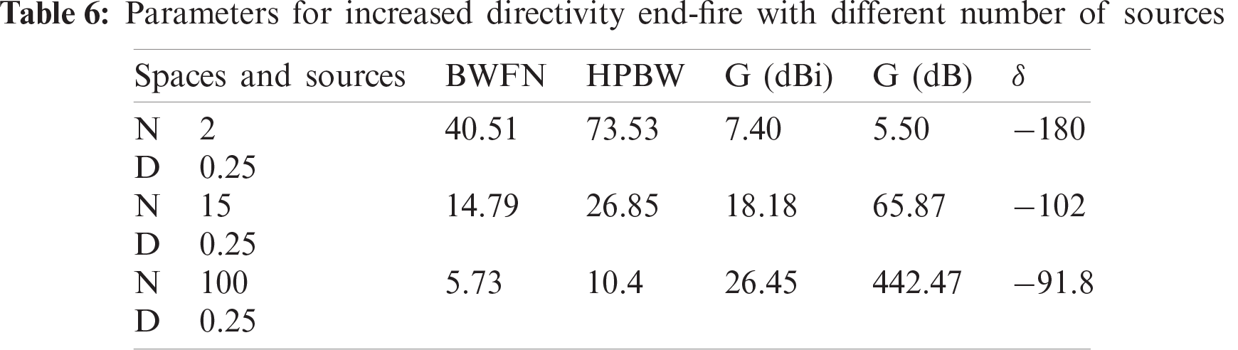
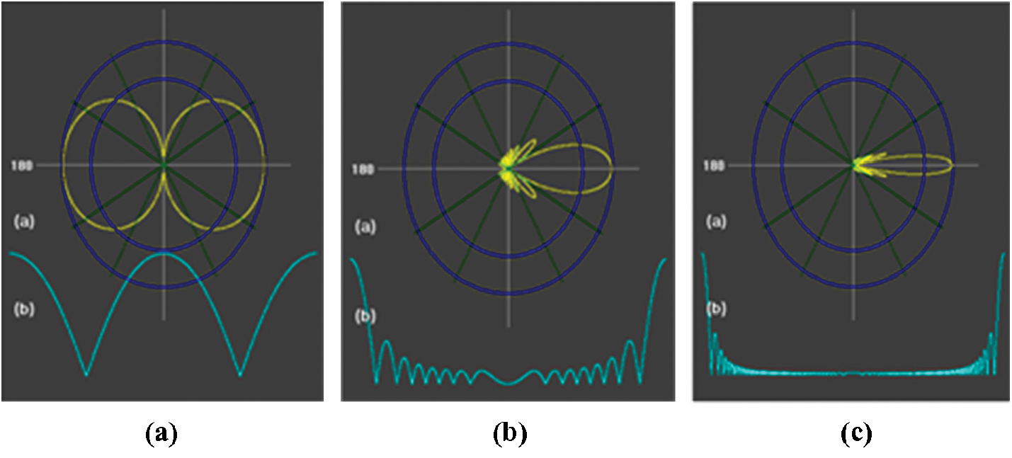
Figure 14: The perfect case for increased directivity end –fire with: (a) (N = 2) and (D = 0.25), (b) (N = 15) and (D = 0.25), and (C) (N = 100) and (D = 0.25)
The antenna array's engineering design process is very similar to the filter synthesis process because the array is synthesized. Signal processing in the antenna array analysis and synthesis requires a set of tools based on MATLAB digital computing environment to obtain the radiation pattern. The synthesis of multiple and different patterns is one of the most important characteristics of antenna arrays. This makes its results almost infinite, as each element is enthusiastic with the other with an identical signal on one hand and on the other hand to obtain the signal processing and radiation pattern processes, which are a wide range of instruments from the signs in the antenna for array analysis, based on the assumption of a narrow band. For several reasons it is difficult to comprehend because they depend on each other (main or partial dependence). On the other hand, the radiation pattern may be useful, but lateral lobes or profit factors and the other parameters determine the radiation pattern. Etc. may not be appropriate for what is stated or required for this environment or problem. We found that rising the value of the phase angle has a very significant and beneficial role because of the beam from the array, so when shifting the phase (phase gradient) in the paths of the elements from the array and inserting it electronically so that the phase shifters can be used, it will be handy to direct the beam in better and customized directions.
The process design simulation aims to study each type of antenna and choose the best style for ideal coverage. We obtained several results for each antenna so that each antenna was distinguished from the other, according to the type of request or the type of problem in the quality of coverage. The synthesis of multiple and different patterns is one of the essential characteristics of antenna arrays. This makes its results almost infinite. The most important results can be summarized as the Broadside array was used to see the effect of space on the pattern field when the distance between the sources is equal to 0.25 λ. When space increases up to 0.25 λ, the half-power beamwidth decreases and appears side lobes. In the ordinary end-fire array, the half-power beamwidth is complete; we used this type when the regional coverage is open because the radiation pattern does not meet obstructions. The increased directivity End-fire array uses this type when the local coverage does not contain the desired range. It is the sea or dissent.
Funding Statement: The authors extend their appreciation to the Deanship of Scientific Research at King Khalid University for funding this work under Grant Number (RGP 2/25/42), Received by Fahd N. Al-Wesabi. https://www.kku.edu.sa.
Conflicts of Interest: The authors declare that they have no conflicts of interest to report regarding the present study.
1. Y. Ma, J. Wang, Y. Li, M. Chen and Z. Li et al. “Smart antenna with automatic beam switching for mobile communication,” Journal of Wireless Communication Network, vol. 179, pp. 1–19, 2020. [Google Scholar]
2. C. Joseph and S. Theodore, Smart Antennas for Wireless Communications: Is-95 and Third Generation CDMA Applications, 1st ed., New York: Pearson College Div., 2015. [Google Scholar]
3. Q. Luo and S. Gao, “Smart antennas for satellite communications,” in Handbook of Antenna Technologies, Singapore: Springer, pp. 1–32, 2015. [Google Scholar]
4. M. A. Almekhlafi, “Analytical study for measuring the electromagnetic radiation of the GSM system in urban areas,” International Journal of Computer Networks & Communications, vol. 9, no. 1, pp. 39–53, 2017. [Google Scholar]
5. V. Midasala, and P. Siddaiah, “Microstrip patch antenna array design to improve better gains,” Int. Conf. on Computational Modeling and Security, vol. 85, pp. 401–409, 2016. [Google Scholar]
6. M. A. Almekhlafi, “Analytical study to assess the performance and quality GPRS network for some of the cells in sana'a,” International Journal of Computer Networks and Communications Security, vol. 4, no. 11, pp. 309–315, 2016. [Google Scholar]
7. B. Gross, Smart Antennas with MATLAB®, 2nd ed., New York: McGraw-Hill Education, 2015. [Google Scholar]
8. R. L. Haupt, Antenna Arrays: A Computational Approach, USA: Wiley & Sons, Inc., 2010. [Google Scholar]
9. M. Patel, P. Kuchhal, K. Lal and R. Mishra, “Design and analysis of microstrip patch antenna array using different substrates for x-band applications,” International Journal of Applied Engineering Research, vol. 12, no. 19, pp. 8577–8581, 2017. [Google Scholar]
10. V. Inzillo, F. De Rango, L. Zampogna and A. Quintana, “Smart antenna systems model simulation design for 5 g wireless network systems,” in Array Pattern Optimization, London: IntechOpen Compacts, 2018. [Google Scholar]
11. S. Hawar, “Measurement-based analysis and evaluation of performance of mobile phones base stations antenna,” in IEEE Int. Conf. on Computational Intelligence & Communication Technology, US, pp. 229–234, 2015. [Google Scholar]
12. T. Huang, P. Pan and H. Hsu, “Adaptive beam steering smart antenna system for ultra-high-frequency radio frequency identification applications,” in Int. Sym. on Computer, Consumer and Control, Taichung, pp. 713–716, 2012. [Google Scholar]
13. C. Gu, S. Gao, H. Liu, Q. Luo, T. Loh et al., “Compact smart antenna with electronic beam-switching and reconfigurable polarizations,” IEEE Trans. Antennas Propag, vol. 63, no. 12, pp. 5325–5333, 2015. [Google Scholar]
14. A. B. Guntupalli and K. Wu, “60 GHz Circularly-polarized smart antenna system for high throughput two-dimensional scan cognitive radio,” in IEEE MTT-S Int. Microwave Sym. Digest, Seattle, pp. 1–3, 2013. [Google Scholar]
15. D. Salama, M. N. Abdallah, T. K. Sarkar and M. Salazar-Palma, “Smart non-uniform antenna arrays deployed above an imperfect ground lane at multiple frequencies,” in IEEE-APS Top. Conf. Antennas Propag. Wirel. Commun. APWC, Italy, vol. 2017, pp. 292–295, 2017. [Google Scholar]
16. S. Kalra, R. Datta, B. S. Munjal and B. Bhattacharya, “Smart reconfigurable parabolic space antenna for variable electromagnetic patterns,” IOP Conf Ser Mater Sci Eng, vol. 311, no. 1, pp. 1–8, 2018. [Google Scholar]
17. A. Singh, J. Kyllonen, S. Caduc, J. Shamblin, M. Garg et al., “Compact smart antenna system for improving probability of detection,” in IEEE Int. Sym. on Antennas and Propagation & USNC/URSI National Radio Science Meeting, San Diego, pp. 1383–1384, 2017. [Google Scholar]
18. X. Wang and E. Aboutanios, “Reconfigurable adaptive linear array signal processing in GNSS applications,” in IEEE Int. Conf. on Acoustics, Speech and Signal Processing, Vancouver, pp. 4154–4158, 2013. [Google Scholar]
19. X. Wang, E. Aboutanios, M. Trinkle and M. G. Amin, “Reconfigurable adaptive array beamforming by antenna selection,” IEEE Trans. Signal Process, vol. 62, no. 9, pp. 2385–2396, 2014. [Google Scholar]
20. Z. Li, E. Ahmed, A. M. Eltawil and B. A. Cetiner, “A beam-steering reconfigurable antenna for WLAN applications,” IEEE Trans. Antennas Propag, vol. 63, no. 1, pp. 24–32, 2015. [Google Scholar]
21. D. Kurita, K. Tateishi, A. Harada, Y. Kishiyama, S. Itoh et al., “Indoor experiment on 5G radio access using beam tracking at 15 GHz band,” in IEEE 27th Annual Int. Sym. on Personal, Indoor, and Mobile Radio Communications, Valencia, pp. 1–6, 2016. [Google Scholar]
 | This work is licensed under a Creative Commons Attribution 4.0 International License, which permits unrestricted use, distribution, and reproduction in any medium, provided the original work is properly cited. |