DOI:10.32604/cmc.2021.018260
| Computers, Materials & Continua DOI:10.32604/cmc.2021.018260 | |
| Article |
Toward Robust Classifiers for PDF Malware Detection
College of Computers in Al-Leith, Umm Al Qura University, Makkah, Saudi Arabia
*Corresponding Author: Marwan Albahar. Email: mabahar@uqu.edu.sa
Received: 03 March 2021; Accepted: 19 April 2021
Abstract: Malicious Portable Document Format (PDF) files represent one of the largest threats in the computer security space. Significant research has been done using handwritten signatures and machine learning based on detection via manual feature extraction. These approaches are time consuming, require substantial prior knowledge, and the list of features must be updated with each newly discovered vulnerability individually. In this study, we propose two models for PDF malware detection. The first model is a convolutional neural network (CNN) integrated into a standard deviation based regularization model to detect malicious PDF documents. The second model is a support vector machine (SVM) based ensemble model with three different kernels. The two models were trained and tested on two different datasets. The experimental results show that the accuracy of both models is approximately 100%, and the robustness against evasive samples is excellent. Further, the robustness of the models was evaluated with malicious PDF documents generated using Mimicus. Both models can distinguish the different vulnerabilities exploited in malicious files and achieve excellent performance in terms of generalization ability, accuracy, and robustness.
Keywords: Malicious PDF classification; robustness; guiding principles; convolutional neural network; new regularization
Malware remains a hot topic in the field of computer security. It is employed by criminals, industries, and even government actors for espionage, theft, and other malicious endeavors. With several million new malware strains emerging daily, identifying them before they harm computers or networks is one of the most pressing challenges of cyber security. Over the last 20 years, hackers have continuously discovered new forms of attacks, giving rise to numerous malware types. Some hackers have utilized macros within Microsoft Office documents, while others have found code in JavaScript files via which browsers were vulnerable. The implication of the range of malware is the necessity of novel automated technology for addressing these attacks. A popular form of the document file is the Portable Document Format (PDF). Although users were unaware, the PDF was transformed into a significant attack vector (AV) for malware operators. Each year, many vulnerabilities are revealed in Adobe Reader, the most widely used software for reading PDF files [1], enabling hackers to commandeer targeted computers. There are three primary forms of PDF malware: exploits, phishing, and misusing PDF capability. Exploits work by exploiting bugs in the API of the PDF reader application, allowing hackers to run code on an attacked computer. This is typically achieved using JavaScript code embedded within files. In phishing attacks, the PDF file itself is harmless, but it requests users to click on a link(s) that exposes the user to an attack. Campaigns of this type have recently been uncovered [2] and are considerably more challenging to recognize because of their format. Misusing PDF capabilities entails exploiting PDF file functionality, e.g., running commands or launching files. Each of these attack types may result in severe outcomes, e.g., hackers stealing website credentials or persuading victims to download malicious executables. Although researchers have recently begun using machine learning to detect malware, antivirus software manufacturers have primarily focused on detecting malicious PDFs using handwritten signatures. This approach demands a considerable investment in human resources and is typically weak at recognizing novel variants and zero-day exploits [3]. An alternative and widely used approach is to perform dynamic analysis by executing files within controlled sandbox environments [4], making the detection of new malware far more likely. However, it also takes considerably longer and requires a sandbox virtual machine. Furthermore, such techniques still need human intervention to define the rules of detection based on the behavior of the files.
Consequently, feature engineering improvements in the design of malicious PDF classifications are challenging but have a substantial and significant impact in the domain. Several approaches have been proposed to improve the robustness of classification algorithms and reduce the evasion rate of malicious files. However, new attack techniques have been quickly developed to evade these approaches. Therefore, propose several models for enhancing the robustness in the detection of malicious PDF files.
In this study, two different classification models are trained to detect malicious and benign PDF files. The dataset utilized in this study was obtained from the VirusTotal and Contagio platforms. In previous research [5,6], the data used for training the algorithms is approximately one-third or less the size of the data used in this study. Using small datasets decreases the generalizability of the training model, which underfits the data and yields ambiguous results. Furthermore, the algorithm designed by He et al. [5] achieved an accuracy of more than 98%, with imbalanced data having a higher proportion of malicious data over benign data.
Consequently, it fails to deliver the same detection performance with a balanced dataset. Falah et al. [6] incorporated a balanced dataset containing approximately 1,000 PDF files. However, the performance of that model is lower than 98%. To detect malicious PDF files, we incorporated a new regularization method based on the standard deviation of the weight matrix in a convolutional neural network (CNN) and an ensemble model based on a support vector machine (SVM) trained for the same purpose. We used more than 50% of the sourced data for training and testing, which increased the detection performance and robustness of the model. To avoid ambiguity and discrepancy in the simulation results, the datasets used for training and evaluating the machine learning models are balanced. Finally, both models perform well, but the proposed CNN-based model produces higher performance measures than state-of-the-art models.
The rest of this paper is organized as follows: In Section 2, we briefly discuss PDF file structure and evasion techniques. In Section 3, we present related research. The dataset used is presented in Section 4, and the methodology is presented in Section 5. We discuss the regularizer used in this study in Section 6 and introduce the system model in Section 7. An extensive analysis of the results is presented in Section 8, a comparison to other models in Section 9, and in Section 10, we explain the limitations of the study. Finally, we present the conclusions and future research directions in Section 11.
The PDF comprises four sections: header, body, cross-reference table, and trailer. Each section provides different information about the file. For example, the file format and version are identified in the header section and with a magic number. While the body section comprises different objects (Fig. 1), the object types include but are not limited to arrays, dictionaries, and name trees. The object type and its content can significantly facilitate the classification of the objects. For instance, JavaScript code is contained within a JS or JavaScript object, as required by the PDF standards. Attackers repeatedly target this object maliciously, and the previous conceptual methods for detecting these attacks were by finding the JS and JavaScript objects. However, the new trend adopted by attackers is to hide JavaScript in indirect objects of various types.
Further, the new trend of hiding malicious code requires the classifier to scan all objects, as was done in the study by Raff et al. [7]. The direct application of n-gram analysis to the entire file disregards the fact that the object content for each form differs significantly, resulting in a lack of robustness. The alternative is to include more semantic information in classification models trained at a higher granularity level. Therefore, training an abnormal classifier essentially achieves this because there is a considerable difference between the content of objects [7].

Figure 1: Tree structure and content of a PDF file
2.2 Classical Antivirus Models for PDF Files
Manufacturers of antivirus software employ several methods for detecting PDF malware. Signature-based detection is the simplest and most frequently used method for identifying malicious files [8]. In this method, a security analyst manually inspects malicious files, extracting one or more patterns in the byte code (the signatures), which are stored in a database. When faced with new files, the analyst checks whether any code in the new files matches codes in the database. If there is a match, the file is blocked. Another essential way of detecting malware is static analysis. In this technique, heuristic rules are applied to the content of the file to assess the likelihood of malware being present. The simplest way of doing this is to search for specific keywords, such as GoTo, JavaScript, or Open-Action, which are tags that can be used to harm a computer system. If none of these tags are present, the analyst gives the file a pass [9] (though certain attackers can now insert JavaScript codes without a matching JavaScript tag). Dynamic analysis is a more costly but possibly more robust means of identifying malware. This technique requires files to be run within a controlled environment (sandbox), in which API calls are evaluated and retrieved while checking the network for activity created by potential malware. Programs can then apply a heuristic approach using activity logs, e.g., launching some of the processes for connecting with malicious websites [9].
2.3 PDF Malware Classifiers and Evading Techniques
In this subsection, we examine a pair of open-source PDF malware classifiers that have received a good deal of attention from security analysts: PDFrate [10] and Hidost [11].
• PDFrate [8] employs 202 elements, including counting for multiple keywords and fields within the PDF. For example, checking how many characters there are in the author field, checking how many endobj keywords there are, checking the total number of pixels in all images, and checking the number of JavaScript Mark occurrences. This is done using a random forest classifier, which is 99% accurate and returns 0.2% false positives compared to the Contagio malware dataset [12]. Basic manipulation of a PDF file can cause extremely significant alterations to the feature values in PDFrate. One example would be adding pages from untampered documents to PDF malware, increasing the page count feature to the maximal integer value. This influences numerous other counts.
• Hidost [11] employs bag-of-path features harvested from the parsed tree structure of the PDF. This finds the shortest structural path to every object, including the terminals and non-terminals within the tree, employing binary counts for the paths as features. Research is undertaken only for paths appearing in a minimum of 1,000 files within the corpus, reducing the number of paths from 9,000,000 to 6,087. Evaluation of the Hidost has been done using an SPM model and a decision tree model. These models both boast 99.8% accuracy, with under 0.06% of false positives returned. The binary bag-of-path features can find the input conjointly with the classifier if some specific attack properties are present.
Nevertheless, quantifying the relationship between class labels and selected features with a high correlation with the labels used in the training process is preferred. It is easy to satisfy this preference with standard classification tasks that do not suffer from malware attacks. It is possible to simply employ highly correlated features to establish highly accurate classification models. The problem is that certain features have low correlations with class labels. Within this context, the selected features used by Hidost and PDFrate frequently have high correlations at low-level relationships with class labels. Manual analysis has shown that such features do not necessarily have a causal relationship with the degree of maliciousness of a PDF file. Consequently, accuracy rates fall swiftly when attacks occur, despite such techniques boasting accuracy rates of over 99%. In contrast, features like shellcode occurrences, heap spray, and JavaScript confusion have robust causal relationships with the degree of maliciousness of the sample, as required for functional implementation. It can be problematic to directly discover features that possess robust causal relationships with class labels but removing features with low relationships is straightforward. In practical terms, causal feature selection requires a comprehensive analysis of the samples [5,13].
2.4 Evading Malware Classifiers Automatically
Several automated attacks have found ways to successfully evade PDF malware classifiers using various threat models.
• White-box attacks, it is generally assumed that the attackers have 100% knowledge of a system. Thus, they can directly attack the precise model under training, e.g., gradient-based attacks [14,15]. One example in a white-box environment is the Gradient Descent and Kernel Density Estimation (GD-KDE) attack, which targets the SVM version of PDFrate [15]. Furthermore, Grosse et al. [16] employed an approach that simply adds features to preserve the extant malicious functions of the adversarial malware example [17]. A problem with white-box gradient-based attacks is that instances of evasion are revealed within the feature space such that the PDF malware is not actually generated.
• With a black-box attack, it is generally assumed that the attackers have no access to the parameters of the model. However, they do have oracle access to prediction labels with certain samples and access to prediction confidence in certain instances. In specific environments, the assumption is also made that the model type and features are also known. Xu et al. [18] employed genetic evolution algorithms for the automatic invasion of Hidost and PDFrate. This evolutionary algorithm employs fitness scores for feedback, guiding the quest for difficult to find PDF variants through seed PDF malware mutations. For each generation of the population in the search, the attack employs cuckoo oracles to make dynamic checks confirming whether mutated PDFs retain their malicious functions. Such checks are far more robust than the static insertion-only techniques employed in gradient-based attacks. Dang et al. [19] employed a more constrained threat model that does not give classification score access to attackers, only allowing access to classified labels and black-box morphs for PDF manipulation. They employed the hill-climbing scoring function to attack the classifier using these assumptions.
The signature-based detection method was the standard in cybersecurity, and for the average researcher, it was the method of choice for spotting malicious PDFs [20]. However, there are now more obstacles due to the rapid rise in threats, increasing the effort required for handwritten rules, and the recent pervasiveness of machine learning detection capabilities. Cross et al. [21] performed an analysis of static and dynamic PDF files and proposed a specific set of characteristics for exploring potential harmful actions by PDF files. Those characteristics include launching a program, responding to a user action, running JavaScript, and describing the file format via the presence of an xref table or the number of pages. Cross et al. trained a decision tree classifier on a small dataset of 89 malicious and 2677 benign samples. Thus, they detected approximately 60% of the malware with a precision of 80% on 5-fold cross-validation. Smutz et al. [22] researched the metadata and structure of documents using the feature extraction method. The intended structural features are the number of specific indicative strings (/JS, /Font) or the position of some objects in the file. The higher-level characteristics of the file indicate the metadata features, e.g., when the unique identifier (pdfid0) of the PDF is not a match. Smutz et al. built a random forest classifier with 10,000 files as the training set, 100,000 files (297 malware) as the operational dataset, and 202 manually selected features. Running the training set through 10-fold cross-validation, the results are larger than 99% without any false positives. Furthermore, they performed a malware classification with a false positive rate (FPR) of only 0.2% with that test set. However, these results may cause severe overfitting of the model. A downside of the overfitting problem when running 10-fold cross-validation with random sampling is that it increases the probability of matching files at each iteration for both the training and test sets. Additionally, counting the /Font string as a significant feature of the model may facilitate finding matching files because of a rise in their variance. Tzermias et al. [23] utilized static analysis features, simulating the JavaScript code in the file and detecting 89% of malware in their test dataset. While this approach is powerful to cause confusion, it takes 1.5 s to run the algorithm on a single PDF file, and it requires a vector machine (VM). Zhang [24] recently developed a detection method superior to eight antiviruses in the market using a large dataset containing more than 100,000 files with 13,000 malwares. His detection method entails running a multi-layer perceptron (MLP) on 48 manually selected features, and the achieved detection rate is approximately 95%, with an 0.1% FPR. Usually, a PDF reader requires a predefined set of keywords (tags) in the file content to render services, such as displaying links, opening images, and executing actions. Alternatively, Maiorca et al. [25] produced features using keywords. They specify how to select the incorporated features in three basic steps: First, split the dataset into benign and malicious samples. Second, use a K-Means clustering algorithm to divide the tags into frequent and infrequent sets. Lastly, merge the frequent tags of both classes and begin using them as features. When they applied these steps to a dataset of 12,000 files, they generated 168 features. Using a test set of 9,000 files, they trained a random forest classifier and achieved a detection rate of 99.55% with 0.2% FPR. The results are perfect and similar to those of previous studies. Still, there is a high risk of overfitting from the random splitting of the data and the test malware when they are not necessarily older than the training data. This is commonplace when malicious files use JavaScript of ActionScript exploits. Thus, we can determine the outcome success rate by detecting those two tags. Similar to Extensible Markup Language (XML), PDF displays a hierarchical structure. Šrndić et al. [26] proposed a new method based on an open-source parser to recover the file's tree-like structure. Their method constructs the feature by concatenating all the tags and mapping the path from the root to a tree leaf rather than using a single tag to make the feature. Subsequently, training a decision tree and an SVM model, the paths alone are observed more than 1,000 times in the dataset. The evaluation step was performed using a large dataset of 660,000 files, including 120,000 malwares obtained largely from the VirusTotal platform. The process of obtaining data involves conducting a few experiments over different periods. The researchers used over four weeks of VirusTotal data to train their algorithm during that study and repeated the experiment six times for evaluation. Overall, they obtained a detection rate of 87% with an 0.1% FPR. There is a necessity for prior domain knowledge to use those approaches due to the reliance on manual feature selection or the parsing of the PDF structure. Recently, Jeong et al. [27] applied a CNN directly to the byte code to detect malicious streams inside PDF files. Their methodology is based on utilizing the embedding layer at the top of their neural network to transform the first 1,000 bytes of a stream into vectors. Next, they used more standard machine learning methods to train multiple networks and then compared them, resulting in a detection rate of 97% and a precision of 99.7%. However, this experiment raises several concerns. First, Jeong et al. limited the search with the convolutional filters to focus on a specific string with JavaScript, a small dataset of 1,978 streams, all containing malicious streams with JavaScript embedded.
Additionally, instead of comparing the networks with tag-level feature extraction, as described previously, their standard only compares the networks with other machine learning models at the byte level. Over the last few years, there have been many attempts to apply deep learning in detection, especially in detecting malware in executable files (type exe). David et al. [28] exploited the behavior of executables to automatically produce signatures using a deep belief network with denoising autoencoders. They extracted API calls and produced 5,000 one-hot encoded features from them by running the files in a sandbox. The resulting output of the classifier network was signatures containing 30 features, achieving 98.6% accuracy with the dataset used. Pascanu et al. [29] advanced the use of deep learning on API calls. They used an echo state network and a recurrent neural network to embed the malware behavior. In the network training phase, they predicted the next API call and determined the features of a classifier from the last hidden state. They achieved a detection rate of 98.3% with an 0.1% FPR. Saxe et al. [30] used static analysis of executable files to manually extract features. This analysis is performed using a four-layer perceptron model and detects 95% of the malicious files in their dataset with 0.1% FPR.
Regarding applications that use CNNs, Raff et al. [31] utilized a CNN to detect malicious executables on raw bytes. Their methodology extracts the matrix as an input to the CNN from the embedding layer and then converts the first bytes of the file into a matrix. Essentially, they obtained their dataset from two different sources, and it has more than 500,000 files. Raff et al. achieved 90% balanced accuracy. While the resulting outcome is clearly inferior to that of the other approaches, their approach does not require preprocessing of the data and yields efficient predictions. Accuracy is enhanced by 1.2% with the inclusion of more training files (two million).
Based on this literature review, there are various proposed methods for malicious PDF detection, including machine learning methods, and these approaches achieve satisfactory results with traditional datasets. However, as long as there is a continued evolution of the machine learning models used by attackers and defenders, it is certain that new and more advanced adversarial strains will be produced that evade existing detectors. Therefore, the creation of stable detection models with robust classification efficiency is an open challenge.
A malicious PDF document primarily uses JavaScript for cyberattacks; therefore, every malicious PDF document contains JavaScript codes in some form. However, JavaScript is seldom found in legitimate documents. However, it could lead to overfitting if JavaScript alone is used as the basis for detection because some legitimate documents contain JavaScript. According to Falah et al. [6], a dataset includes various types of attacks, including PowerShell downloaders, URL downloaders, executable malware, and shellcode downloaders. To encompass all of these attack classes, we obtained all modern malicious documents provided by the VirusTotal and Contagio datasets, as discussed subsequently.
In this study, the dataset used was obtained from two different sources:
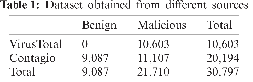
1. VirusTotal: There are 10,603 malicious files sourced from this platform, obtained in December 2017.
2. Contagio [32]: There are a total of approximately 20,000 malicious and clean PDF files sourced from this platform, obtained in November 2017.
More than 30,000 files were used in this study for the training of different machine learning models. The distribution of benign and malicious files is presented in Tab. 1.
5.1 Feature Extraction from Object Content Based on Encoding and N-Gram
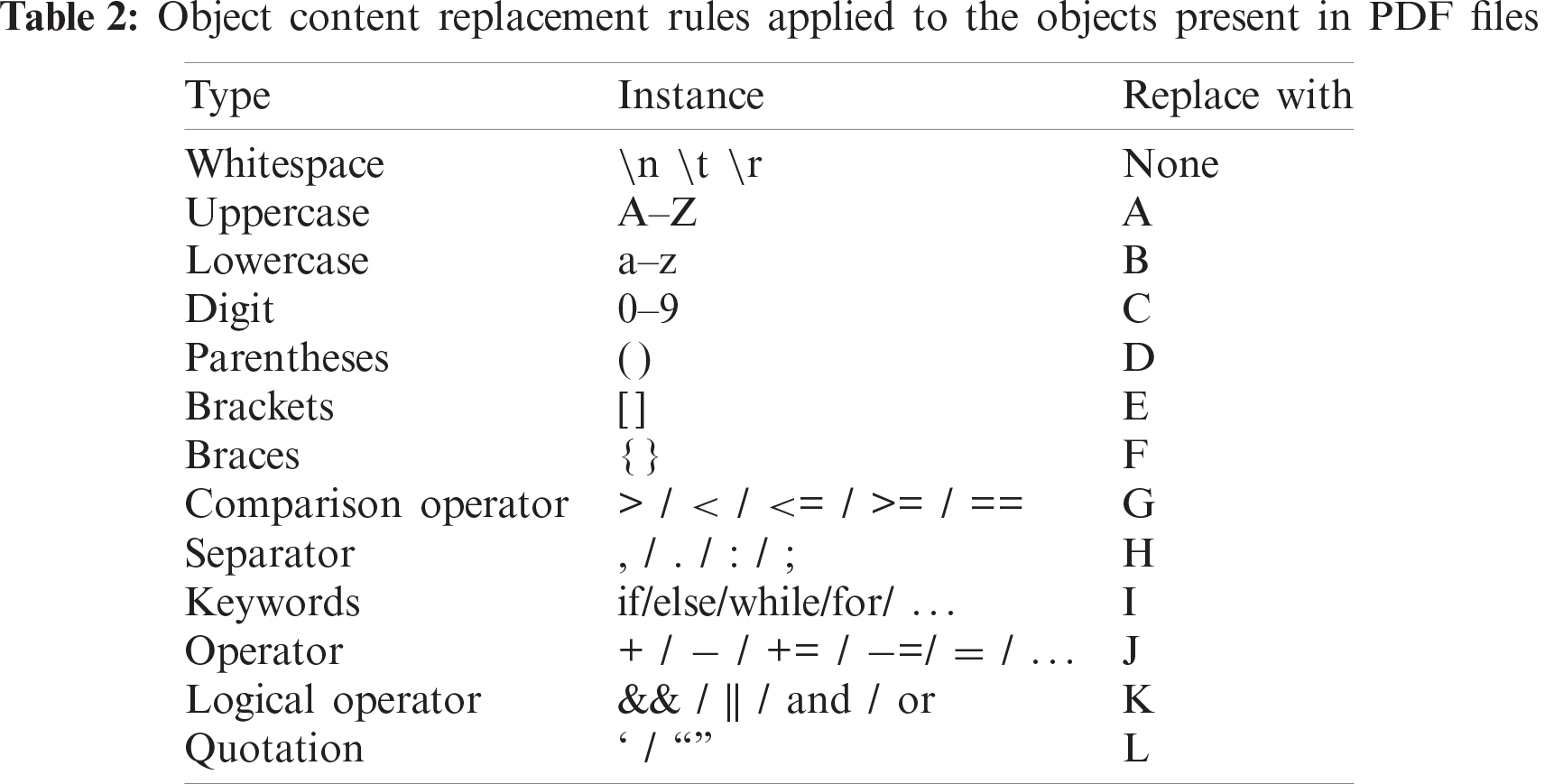
The n-gram analysis cannot be applied directly for our purposes because it increases the space occupied by the features, making it difficult to execute the process of selecting features. Furthermore, it increases the sensitivity of features that eliminate the stability and robustness of the model, paving the way for evasion through simple code confusion. Such issues are overridden via object content replacement based on the object type. These principles are based on the dependence of neighboring types rather than specific characters. For example, a JavaScript code such as Doc = DocumentApp.openById (“<my-id>”) can be replaced with ABBGABBBBBBABBHBBBABABDLGBBJBBGLD. After this encoding, the number of unique elements is reduced to less than 30 (Tab. 2). Similarly, the respective features are less sensitive to modification due to code confusion and encoding. Not only does it improve robustness, but it also makes it easy to reduce the feature dimensions.
Similar to the study by He et al. [5], the feature extraction method is applied to a benign dataset, and then abnormality is performed. The steps of the feature extraction based on encoding and n-gram are as follows:
1. PDF files are parsed and extracted.
2. Depending on their type, objects are added to different datasets.
3. The respective objects are decoded and decrypted as string content based on the PDF format specifications for each dataset.
4. Encoding is performed (Tab. 2 [5]), and the feature set is generated using the n-gram approach.
5. Frequencies are computed for feature occurrence and passed through a threshold to filter out features with fewer occurrences and negligible effects.
6. The final features dataset is created by combining all the features extracted in Step 1 to Step 2 and fed into the machine learning model.
5.2 Feature Extraction Based on the File Structure
A PDF file can be represented by a tree-like structure, with each node representing different objects in the file. In this study, we incorporated both the horizontal and vertical relationships among the objects mentioned by He et al. [5]. Our task is to classify malicious and benign PDF files based on the information present in these files; therefore, objects in PDF files were organized in an adjacency matrix that captures the file structure, which is also called a structure matrix. The process of extracting features based on the file is given below:
1. PDF files are parsed, and different objects are extracted.
2. Low-frequency types are filtered out.
3. Both benign and malignant types are combined.
4. The feature matrix and feature values are generated by combining objects with similar names based on functionality.
Further, the same process described by He et al. [5] is applied. The features extracted using object encoding and the n-gram were used to train the k-mean clustering model for each object type to detect abnormal objects. In parallel, the structure matrices were computed and further extended by adding new dimensions, showing the intermediate results for the respective types. These extended structure matrices were used to train the CNN model embedded with the new regularization, as explained in the following sections.
The primary consideration with machine learning is that an algorithm can be created that works efficiently, both with training data and with new data. The “no free lunch” theorem suggests that every individual task requires a machine learning algorithm’s customized design. Learning machines have collections of incorporated preferences and strategies suited to tuning the problem they are addressing. Such preferences and strategies aimed at the central objective of improving generalization are together referred to as regularization. With deep learning, various regularization methodologies are now accessible due to the substantial quantity of parameters involved. Most of the research in recent years has been devoted to developing regularization strategies that work more effectively.
With machine learning, data sample points can be divided into two components: a pattern and stochastic noise. All machine learning algorithms must have the capability to model the pattern while ignoring the noise. Machine learning algorithms that stress finding a fit for the noise and other peculiarities will tend toward overfitting along with the pattern. In such instances, regularization can help select a suitable level of model complexity for improving the algorithm’s predictions.
In general, there are dangers of overfitting with complex models that have no training errors and high testing errors. On occasion, it is preferable to have robust false assumptions rather than weak correct assumptions because weak correct assumptions require additional data to prevent overfitting. Overfitting can occur in several ways and is not always easily identifiable. One means of understanding overfitting is the decomposition of generalization errors into variance and bias.
6.1 Lasso Regression (L1) Regularization
An L1 regularizer [33] imposes penalties on the absolute values of the weight matrix to prevent it from reaching a higher value. The primary advantage of the L1 regularizer is that it imposes a weight value reduction to zero for less significant features, which are not required for the definition of classifier boundaries but are selected or reduced by the L1 regularizer. Eq. (1) demonstrates that the absolute size of a regression coefficient has been penalized. The L1 regularizer can also implement reductions in variability and improve the accuracy of a linear regression model. This regularizer is notated mathematically as follows
where n is the number of features within the dataset,
However, if the predicted numbers exceed the observed numbers, the L1 regularizer will select, as a maximum, n predictors as non-zeros, even when every predictor has relevance (or can be employed in the test set). In these instances, the L1 regularizer may have difficulty coping with this form of data. In a case where two or more highly collinear variables are presented, the L1 regularizer regression will choose one of them at random, which is unsuitable for data interpretation.
6.2 Ridge Regression (L2) Regularization
An L2 regularizer [33] introduces modification into the residual sum of squares (RSS) via the addition of a penalty equivalent to the square of the magnitude of the coefficients. However, this is considered a suitable technique only when there is multicollinearity (high correlation between independent variables) in the data. With multicollinearity, although the ordinary least squares (OLS) estimates do not have bias, they have a large variance, which shifts the observed values away from the true values considerably. The addition of an element of bias in regression estimates results in ridge regression, which causes a reduction in quality errors. This generally resolves multicollinearity problems via the shrinkage parameter
where
The L1 regularizer is different from the L2 regularizer because it implies absolute values and not square values for the penalty function. This means that penalties are imposed (or equivalent constraints for the estimated sum of the absolute values), which results in certain parameter estimates being calculated as precisely zero. The higher the applied penalty, the further the estimates shrink in the direction of absolute zero. This facilitates variable selection from a mandated range of n variables.
In the machine learning discipline, the most frequently employed regularization methods are L1-norm and L2-norm. In the optimization discipline, such regularizers assess weight complexity to create a more general mapping in the network. The L1-norm imposes a penalty on the sum of absolute values, while the L2-norm imposes a penalty on the sum of squared values. The new regularization form takes the standard deviation of the weight matrix and multiples it by
where
Next, the mathematical formula for calculating
where k represents the row count, and i is the ith row in the weight matrix.
Hence, we minimize the loss function of
Fig. 2 illustrates the feasible region for L1 and L2 and the new regularization technique. We show the contour of the new regularizer, which highlights its power and effectiveness. The various loss values are represented by the contour of each regularizer. The L2-norm behaves in a circular fashion, incorporating the L1-norm. However, the new regularizer behaves in a parabolic fashion and extends values past the limit of the L2-norm. This is somewhat helpful, as it leads to an increase in the limit values (space) for adoption, and the space may be expanded based on the penalty term

Figure 2: Contours of the L2 (left) and L1 (middle) regularizers and the new (right) regularizer. Here, we demonstrate the coefficients ß1 and ß2 at the global minimum
7 Model Architecture and Training
7.1 Convolutional Neural Network (CNN) Integrated with the New Regularization
The CNN models used in this study have three convolutional layers, inspired by Fettaya et al. [34]. This model is integrated with the new regularization described in the preceding sections. The first convolutional layer has a window size of eight, a stride of two, and 20 kernels. The second layer has the same window size and stride, but the number of kernels is increased to 40.
Similarly, the window size in the last convolutional layer is reduced to four with a stride of two, and the number of kernels is increased to 80. All these layers are immediately followed by a batch-normalization layer, as shown in Fig. 3. Ultimately, 256 fully connected layers and a classification layer are inserted. Furthermore, each convolution layer and the fully connected layers are directly followed by a rectified linear unit (ReLu) in the CNN model.

Figure 3: Proposed CNN architecture based on new regularization
In addition to the neural network model, we trained an ensemble model based on an SVM [35] with three different kernels. The kernel is a popular method used in SVMs to make data more separable and distinguishable while projecting data to higher dimensions. In the first step, the structure matrix (the values of the structure matrix) is flattened to a single dimension with 2,500 elements. The size of the input is restricted to 2,500 as input to the SVM. The types of kernels used in an SVM are explained below.
• Gaussian kernel
The Gaussian kernel is a popular kernel used in SVM. It adds a bump around each data point [35]. Mathematically it can be expressed as Eq. (6).
where
• Polynomial kernel
The polynomial kernel is commonly described as expressed in Eq. (7). It is a directional function with a point product in the kernel that depends on the directions of two vectors in a low-dimensional space.
We considered two SVM classifiers with polynomial kernels of degree d = 2 (SVM-2) and d = 3 (SVM-3). The SVM-based ensemble model is illustrated in Fig. 4.
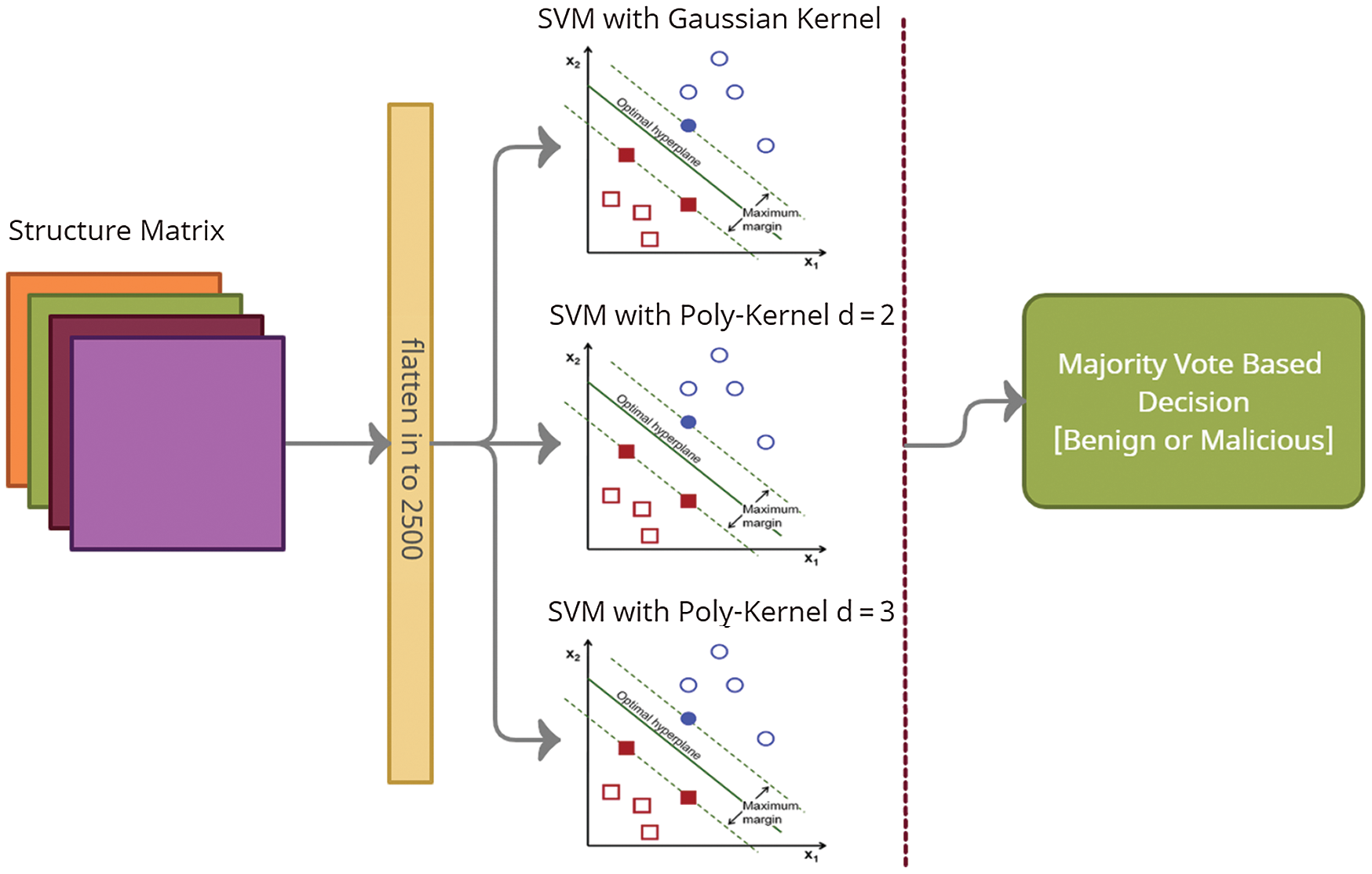
Figure 4: Proposed SVM-based ensemble architecture
7.3.1 Training and Testing of the CNN Model
The CNN model integrated with the proposed regularization method was trained using the features extracted via the methods in the preceding section. There are 30,797 PDF files in the dataset, and 40% of this data (sourced from both the VirusTotal and Contagio datasets), totaling 12,970 PDF files, was used in the training. For testing, 15% disjoint data from both categories were used. To make the dataset nearly balanced, of this 40% used, 60% of the files from the Contagio dataset were benign and 40% were malicious files. Hence, the number of benign and malicious PDF files used for the training was 5,500, and 7,470, respectively. The same ratio was applied to test data from the Contagio dataset.
7.3.2 Training and Testing of the Ensemble Model
The SVM-1, SVM-2, and SVM-3 classifiers were trained and tested in parallel fashion on the data presented in Tabs. 3 and 4. The malicious and benign decision was made based on majority vote. For example, if SVM-1 and SVM-3 called an instance malicious and SVM-2 called it benign, it was considered malicious.
7.4 Hyper-Parameters Adjustment
To train the model effectively, the number of batches is restricted to 64, and the learning rate is initially set to 2
The experiments in this study were performed on a computer system with 64 GB of RAM, four 2.4 GHz Intel CPUs, and a GeForce GTX 1080 TI GPU packed with a massive 11 GB frame buffer.
To evaluate the performance of our model, we computed different evaluation metrics, including accuracy, precision, recall, and F1 score. Each of these metrics is expressed in Eqs. (8)–(11). In these equations, true positives (TP) are the samples correctly classified as malicious, while false positives (FP) are benign samples classified as malicious. Similarly, true negatives (TN) are samples correctly classified as benign, while false negatives are malicious samples classified as benign.
Accuracy is computed as the ratio of correct predictions divided by the total number of predictions (Eq. (8)). The true positive rate (TPR) or recall is derived by dividing the predicted number of malicious samples by the total number of actual malicious samples in the test data (Eq. (9)). Similarly, precision is derived by dividing the predicted number of malicious samples by the number of all samples identified by the classifier as malicious (Eq. (10)). It can be seen from Eqs. (9) and (10) that an increase in precision causes a decrease in recall, and vice versa; hence, the F1 score, which is computed to maintain balance between the two measures (Eq. (11)).
8.2 Prediction Performance of Proposed Models
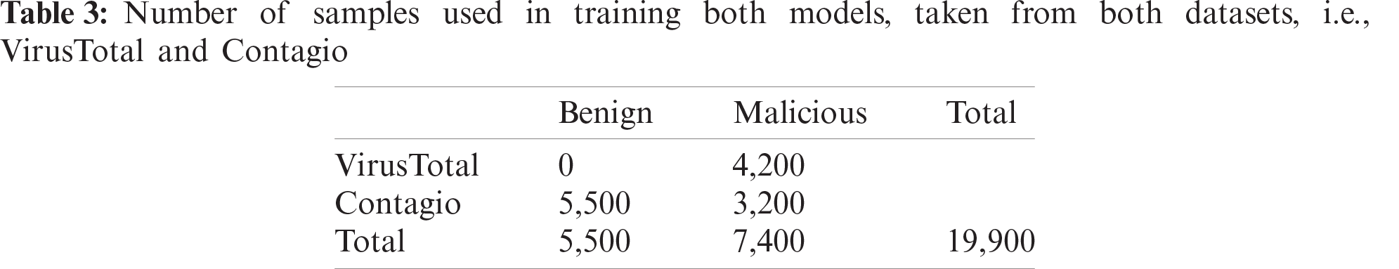
The proposed CNN and ensemble models are trained with over 12,900 PDF files, and the number of benign and malicious files used in the training process is 5,500, and 7,400, respectively. The distribution of the PDF files obtained for training, both the VirusTotal and the Contagio datasets, are presented in Tab. 3.
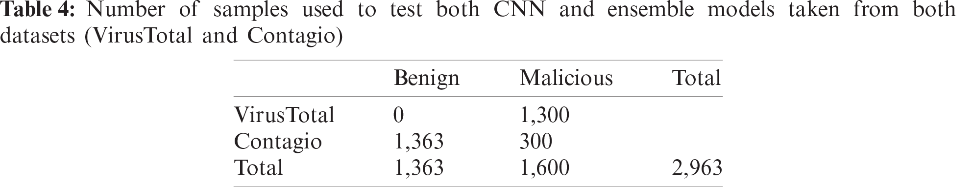
After training, the performance of both models is evaluated using a test dataset. The distribution of the test data from both the VirusTotal and Contagio datasets is presented in Tab. 4. The number of samples is decided such that the test data is almost balanced. The total number of files used for the evaluation of the model is 2,963.
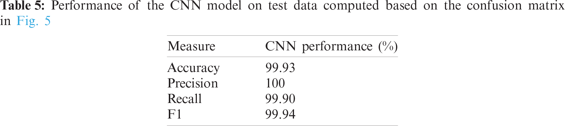
The confusion matrix of the trained CNN model is shown in Fig. 5. The accuracy and precision of the CNN model is almost 100%. The recall and F1 scores are 99.9% and 99.8%, respectively. All measures of the CNN model are presented in Tab. 5.
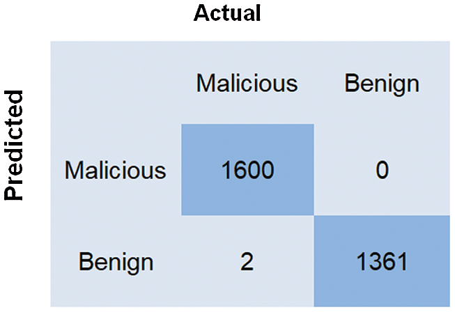
Figure 5: Confusion matrix of the CNN model on the test data
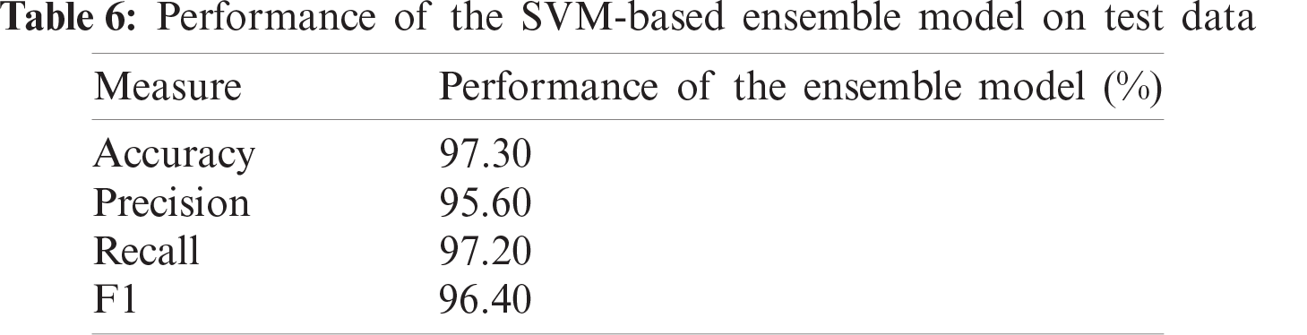
The accuracy of the ensemble model is 97.3%, while the precision and recall are 95.6% and 97.2%, respectively. The relative performance of the SVM-based ensemble model is lower than that of the CNN-based model. This is because the representation power of the neural network based model is higher than that of the other models because of their complexity and learning abilities. The task here is to classify the features and learn from the features where the CNN performs this task easily.
All measures of the SVM-based ensemble model are presented in Tab. 6.
The area under the ROC curve (AUC-ROC) of the CNN model and ensemble model is 99.4% and 94.3%, respectively. Figs. 6 and 7 present the ROC curve of both proposed models.

Figure 6: AUC-ROC of the proposed CNN model
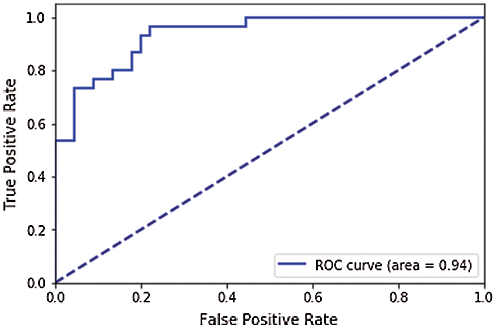
Figure 7: AUC-ROC of the ensemble model
8.3 Comparison of the Proposed Model with Other Models
In this section, the performance of our model in terms of accuracy, recall, precision, and F1 measure is compared with state-of-the-art models from other studies. Our proposed CNN-based model outperforms every other model presented in Tab. 7. The precision of the He et al. [5] model and our proposed model is 100%, while our CNN-based model scores slightly higher on the other measures. The performance of the SVM-based ensemble model is approximately similar to that of the model put forward by Falah et al. [6]. However, the performance of the ensemble model is lower than that of models from other recent studies compared in Tab. 7. A graphical representation of the comparison with the different models is presented in Fig. 8.
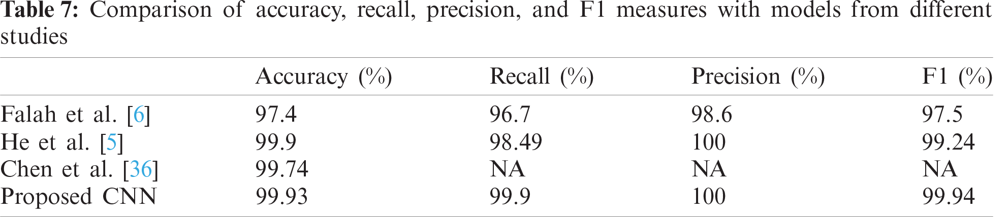

Figure 8: Comparison of Accuracy, Recall, and F1 measures of the proposed CNN model with different state-of-the-art models
To avoid evasion, the robustness of a detection model for malicious PDF documents is indispensable. Therefore, the robustness of the proposed classifier is evaluated using adversarial samples generated via Mimicus, a Python library for adversarial classifier evasion [14].
Because the feature extraction process uses unsupervised learning, the detection process uses supervised learning; therefore, the evasion of the unsupervised model is difficult due to collision resistance in the selected features. However, if the unsupervised model is evaded by the adversarial samples, then the supervised model utilizes the structural information of the input features. Therefore, it would be difficult to evade the proposed model by explicitly or implicitly placing hidden malicious data in the input file.
The workings of Mimicus are based on the set of features, the training data, and the classification algorithm. We generated approximately 30 samples, a similar number as in the study by He et al. [5] and tested our proposed models on these adversarial samples. The results show that all adversarial samples generated under these conditions are detected by the proposed classifiers. In comparison, several state-of-the-art models from the study by Maiorca et al. [37] have shown excellent performance on training samples. However, their performance decreases when tested on adversarial samples generated via Mimicus (testing set) [5]. In the face of adversarial attacks, the performance of our model is superior to that of other state-of-the-art models. It is evident from Fig. 9 that our model detected each adversarial sample 100% correctly.

Figure 9: Robustness accuracy of various models computed using adversarial samples generated vias Mimicus. The accuracy of our proposed model is almost 100%
Various methods have been proposed to detect malicious PDF files with comparable accuracy [5–37], all of which can be integrated into real-time applications. The detection performance of our proposed method is superior to that of other existing methods. Although, there is a feature extraction overhead involved, which might delay the throughput of real-time applications. The two types of feature extraction that make the detection possible with 100% precision are object, content, features, and structure-based features, which are time consuming. However, apart from the time versus precision trade-off, our proposed method can be used in applications where high security is desired against intentionally evasive attacks.
11 Conclusion and Future Directions
In this study, we proposed two models for detecting malicious PDF files. The first model is a CNN model integrated with a new regularization, and the second model is an SVM-based ensemble model with three different kernels. A feature extraction method is used to extract features based on the object content and file structure in the first step. In the next step, two different classifiers are trained to detect malicious documents. Both models were trained and validated using two datasets. The first model possesses an advantage over other regularizations, optimizing weight values based on the standard deviation. It restricts the dispersion of weight parameters, making the conversion fast, preventing overfitting of the model, and improving performance. Thus, the model leverages feature transformation by adding three convolutional layers, yielding promising performance. In addition, the second model yields comparable results. However, the CNN-based model outperforms all the other models.
In the future, the feature extraction methods can be modified to avoid overhead and delay from the various types of feature extraction. In addition to intensive feature extraction methods, another avenue worth exploring is the identification of discriminant features for detecting malicious PDF documents with high accuracy, precision, and greater robustness accuracy.
Funding Statement: This research work was funded by Makkah Digital Gate Initiative under Grant No. (MDP-IRI-16-2020). Therefore, authors gratefully acknowledge technical and financial support from Emirate Of Makkah Province and King Abdulaziz University, Jeddah, Saudi Arabia.
Conflicts of Interest: The authors declare that they have no conflicts of interest to report regarding the present study.
1. Mitre Corporation, “CVE details,” Vulnerability Statistics. 2018. [Online]. Available: https://www.cvedetails.com/product/497/Adobe-Acrobat-Reader.html?vendor_id=53. [Google Scholar]
2. M. Beltov, “PDF phishing scam campaign revealed,” Best Security Search, 2017. [Online]. Available: https://bestsecuritysearch.com/pdf-phishing-scam-campaign-revealed/. [Google Scholar]
3. Dan Goodin, “Anti-virus protection gets worse,” The Register, 2007. [Online]. Available: https://www.theregister.com/2007/12/21/dwindling_antivirus_protection. [Google Scholar]
4. U. Bayer, A. Moser, C. Kuruegel and E. Krida, “Dynamic analysis of malware code,” Journal in Computer Virology, vol. 2, no. 1, pp. 67–77, 2006. [Google Scholar]
5. K. He, Y. Zhu, Y. He, L. Liu, B. Lu et al., “Detection of malicious pdf files using a two-stage machine learning algorithm,” Chinese Journal Electronics, vol. 29, no. 6, pp. 1165–1177, 2020. [Google Scholar]
6. A. Falah, L. Pan, S. Huda, S. R. Pokhrel and A. Anwar, “Improving malicious pdf classifier with feature engineering: A data-driven approach,” Future Generation Computer Systems, vol. 115, no. 2, pp. 314–326, 2021. [Google Scholar]
7. E. Raff, R. Zak, R. Cox, J. Sylvester, P. M. Yacci et al., “An investigation of byte n-gram features for malware classification,” Journal of Computer Virology and Hacking Techniques, vol. 14, no. 1, pp. 1–20, 2018. [Google Scholar]
8. Comodo Antivirus, “How antivirus works,” Comodo Security Solutions, 2020. [Online]. Available: https://antivirus.comodo.com/faq/how-antivirus-works.html. [Google Scholar]
9. P. Singh, S. Tapaswi and S. Gupta, “Malware detection in pdf and office documents: A survey Information Security,” A Global Perspective, vol. 29, no. 3, pp. 134–153, 2020. [Google Scholar]
10. C. Smutz and A. Stavrou, “Malicious pdf detection using metadata and structural features,” in Proc. of the 28th Annual Computer Security Applications Conf., Orlando Florida USA, pp. 239–248, 2012. [Google Scholar]
11. N. Šrndić and P. Laskov, “Detection of malicious pdf files based on hierarchical document structure,” in Proc. of the 20th Annual Network & Distributed System Security Symp., San Diego, California, USA, pp. 1–16, 2013. [Google Scholar]
12. M. Parkour, “Contagio malware dump,” Version 4 April 2011 - 11,355+ Malicious Documents-archive for Signature Testing and Research, 2011. [Online]. Available: http://contagiodump.blogspot.com/2010/08/malicious-documents-archive-for.html. [Google Scholar]
13. L. Tong, B. Li, C. Hajaj, C. Xiao and Y. Vorobeychik, “A framework for validating models of evasion attacks on machine learning with application to pdf malware detection,” arXiv Preprint, 2017. [Google Scholar]
14. B. Biggio, I. Corona, D. Maiorca, B. Nelson, N. Srndc et al., “Evasion attacks against machine learning at test time,” in Joint European Conf. on Machine Learning and Knowledge Discovery in Databases, Berlin, Heidelberg, pp. 387–402, 2013. [Google Scholar]
15. N. Šrndić and P. Laskov, “Practical evasion of a learning-based classifier: A case study,” in IEEE Symp. on Security and Privacy, Berkeley, CA, USA, pp. 197–211, 2014. [Google Scholar]
16. K. Grosse, N. Papernot, P. Manoharan, M. Backes and P. Daniel, “Adversarial perturbations against deep neural networks for malware classification,” arXiv Preprint, 2016. [Google Scholar]
17. D. Arp, M. Spreitzenbarth, M. Hubner, H. Gascon, K. Rieck et al., “DREBIN: Effective and explainable detection of android malware in your pocket,” in Network and Distributed System Security Symp., San Diego, California, USA, vol. 14, pp. 23–26, 2014. [Google Scholar]
18. W. Xu, Y. Qi and D. Evans, “Automatically evading classifiers: A case study on pdf malware classifiers,” in Network and Distributed System Security Symp., San Diego, California, USA, 2016. [Google Scholar]
19. H. Dang, Y. Huang and E. C. Chang, “Evading classifiers by morphing in the dark,” in Proc. of the 2017 ACM SIGSAC Conf. on Computer and Communications Security, New York, NY, USA, pp. 119–133, 2017. [Google Scholar]
20. S. Rautiainen, “A look at portable document format vulnerabilities,” Information Security Technical Report, vol. 14, no. 1, pp. 30–33, 2009. [Google Scholar]
21. J. S. Cross and M. A. Munson, “Deep pdf parsing to extract features for detecting embedded malware,” Sandia National Labs, SAND2011–7982, 2011. [Google Scholar]
22. C. Smutz and A. Stavrou, “Malicious pdf detection using metadata and structural features,” in Proc. of the 28th Annual Computer Security Applications Conf., New York, NY, USA, pp. 239–248, 2012. [Google Scholar]
23. Z. Tzermias, G. Sykiotakis, M. Polychronakis and E. Markatos, “Combining static and dynamic analysis for the detection of malicious documents,” in Proc. of the Fourth European Workshop on System Security, New York, NY, USA, pp. 4, 2011. [Google Scholar]
24. J. Zhang, “Mlpdf: An effective machine learning based approach for pdf malware detection,” arXiv Preprint, 2018. [Google Scholar]
25. D. Maiorca, G. Giacinto and I. Corona, “A pattern recognition system for malicious pdf files detection,” in Int. Workshop on Machine Learning and Data Mining in Pattern Recognition, Berlin, Heidelberg, pp. 510–524, 2012. [Google Scholar]
26. N. Šrndić and P. Laskov, “Detection of malicious pdf files based on hierarchical document structure,” in Proc. of the 20th Annual Network & Distributed System Security Symp., San Diego, CA, USA, pp. 1–16, 2013. [Google Scholar]
27. Y. Jeong, J. Woo and A. Kang, “Malware detection on byte streams of pdf files using convolutional neural networks,” Security and Communication Networks, vol. 2019, no. 6, pp. 1–9, 2019. [Google Scholar]
28. O. David and N. Netanyahu, “Deepsign: Deep learning for automatic malware signature generation and classification,” in Int. Joint Conf. on Neural Networks, Killarney, Ireland, pp. 1–8, 2015. [Google Scholar]
29. R. Pascanu, J. Stokes, H. Sanossian, M. Marinescu and A. Thomas, “Malware classification with recurrent networks,” in 2015 IEEE Int. Conf. on Acoustics, South Brisbane, QLD, Australia, pp. 1916–1920, 2015. [Google Scholar]
30. J. Saxe and K. Berlin, “Deep neural network based malware detection using two dimensional binary program features,” in 10th Int. Conf. on Malicious and Unwanted Software, Fajardo, PR, USA, pp. 11–20, 2015. [Google Scholar]
31. E. Raff, J. Barker, J. Sylvester, R. Brandon, B. Catanzaro et al., “Malware detection by eating a whole exe,” in Workshops at the Thirty-Second AAAI Conf. on Artificial Intelligence, New Orleans, USA, pp. 268–276, 2018. [Google Scholar]
32. Contagio Malware Dump, “External data source,” [Online]. Available: http://contagiodump.blogspot.com.au. [Google Scholar]
33. A. Y. Ng, “Feature selection, l1 vs. l2 regularization, and rotational invariance,” in Twenty-First Int. Conf. on Machine Learning, New York, NY, USA, 2004. [Google Scholar]
34. R. Fettaya and Y. Mansour, “Detecting malicious pdf using CNN,” arXiv Preprint, 2020. [Google Scholar]
35. W. Noble, “What is a support vector machine?,” Nature Biotechnology, vol. 24, no. 12, pp. 1565–1567, 2006. [Google Scholar]
36. Y. Chen, S. Wang, D. She and S. Jana, “On training robust pdf malware classifiers,” in 29th USENIX Security Symp., (virtualpp. 2343–2360, 2020. [Google Scholar]
37. D. Maiorca, B. Biggio and G. Giacinto, “Towards adversarial malware detection: Lessons learned from pdf-based attacks,” ACM Computing Surveys, vol. 52, no. 4, pp. 1–36, 2019. [Google Scholar]
 | This work is licensed under a Creative Commons Attribution 4.0 International License, which permits unrestricted use, distribution, and reproduction in any medium, provided the original work is properly cited. |