Computers, Materials & Continua DOI:10.32604/cmc.2021.018090
Article

Brain Tumour Detection by Gamma DeNoised Wavelet Segmented Entropy Classifier

Simy Mary Kurian1, Sujitha Juliet Devaraj1,* and Vinodh P. Vijayan2

1Karunya Institute of Technology and Science, Coimbatore, India
2Albertian Institute of Science and Technology, Kochi, India
*Corresponding Author: Sujitha Juliet Devaraj. Email: sujitha@karunya.edu
Received: 24 February 2021; Accepted: 21 April 2021

Abstract: Magnetic resonance imaging (MRI) is an essential tool for detecting brain tumours. However, identification of brain tumours in the early stages is a very complex task since MRI images are susceptible to noise and other environmental obstructions. In order to overcome these problems, a Gamma MAP denoised Strömberg wavelet segmentation based on a maximum entropy classifier (GMDSWS-MEC) model is developed for efficient tumour detection with high accuracy and low time consumption. The GMDSWS-MEC model performs three steps, namely pre-processing, segmentation, and classification. Within the GMDSWS-MEC model, the Gamma MAP filter performs the pre-processing task and achieves a significant increase in the peak signal-to-noise ratio by removing noisy artefacts from the input brain image. After pre-processing, Strömberg wavelet transform segmentation is carried out to partition the pre-processed image into a number of blocks based on the features extracted from the image. Finally, the maximum entropy classifier identifies and locates the tumour from the input image based on extracted features with high accuracy and minimal error rate. Using a number of MRI images, experimental evaluation and comparison of the proposed model and existing methods is carried out on the basis of four metrics: peak signal-to-noise ratio, tumour detection accuracy, error rate, and tumour detection time with respect to MRI image size. The proposed model offers superior performance in terms of all four metrics.

Keywords: Gamma MAP filter; Strömberg wavelet transform; maximum entropy classifier

1  Introduction

Magnetic resonance imaging (MRI) is a highly developed medical imaging system that can be used to generate high-quality images of the brain. Accurate and exact classification of brain tumours through MRI has an essential role in clinical diagnosis and choosing the best treatment for the patient. Many researchers have worked towards achieving brain tumour detection in earlier stages of tumour development to improve treatment outcomes but have been unable to improve the brain tumour detection accuracy while also reducing the time complexity. In order to address these problems, machine learning techniques are introduced in this study.

A principal component analysis and normalised GIST descriptor with a regularised extreme learning machine (PCA-NGIST with RELM) classifier was introduced by Gumaei et al. [1] for tumour detection by extracting tumour features from brain images. Although this method proves better for feature extraction, noise removal is not performed, and the method fails to achieve higher accuracy in the detection of tumours. A probabilistic neural network (PNN) classifier was developed by Shree et al. [2] for the identification of brain tumours from MRI images. This technique concentrates on noise removal and combines a discrete wavelet transformation (DWT) with the extraction of textural and gray-level co-occurrence matrix (GLCM) features followed by morphological operations. However, it fails to increase the accuracy for a larger dataset. A multi-atlas segmentation (MAS) method was developed by Tang et al. [3] for MR tumour brain images. The conventional low-rank method produces the recovered image with distorted normal brain regions. The designed MAS method does not use any efficient method to improve the accuracy of tumour detection.

A computerized method developed by Roy et al. [4] implements brain tumour recognition and analysis from MRI images, but the focus on achieving a significant increase in accuracy is neglected. Many researchers have employed machine learning techniques to improve the accuracy for tumour detection. A support vector machine (SVM) classifier was presented by Amin et al. [5], with different cross validations on the features to detect the tumour. This automated method easily differentiates cancerous and non-cancerous cells using MRI of the brain, but the time consumption for brain tumour detection is not minimised. The Berkeley wavelet transformation (BWT) presented by Bahadure et al. [6] is also capable of distinguishing ordinary and irregular tissues from MRI images by means of an SVM classifier. However, it fails to achieve better accuracy for classification. An enhanced convolutional neural network (ECNN) was developed by Thaha et al. [7] for brain tumour segmentation. This automatic segmentation method based on CNN and data augmentation is very effective for brain tumour segmentation in MRI images, which is significant because MRI prevents manual segmentation in a reasonable time, limiting the use of precise quantitative measurements of a part of the tumour during clinical treatment. Although the designed ECNN increases accuracy, it does not consider the time evaluation element.

The triangular fuzzy median filtering method developed by Sharif et al. [8] enhances the quality of images for tumour detection using an extreme learning machine (ELM). Although this method minimises the computational time, it does not achieve a better peak signal-to-noise ratio. An automatic brain tumour diagnosis system with threshold-based segmentation was introduced by Edalati-rad et al. [9]. However, the designed system fails to use unsupervised feature learning for segmentation to perform automatic brain tumour detection. Özyurt et al. [10] introduced a fuzzy C-means with a super-resolution and convolutional neural network (SR-FCM-CNN) approach for tumour detection. However, it lacks efficient classification to enhance the performance of tumour detection.

Rajagopal [11] employed a random forest classifier for brain tumour recognition and segmentation. The classifier consumes more time for tumour detection with less accuracy as compared to proposed method. A local binary pattern (LBP) combined with Gabor wavelet transform (GWT) was introduced by Amina et al. [12] for tumour classification. The designed method fails to enhance the segmentation of the tumour region.

An automated determination of segmentation method was introduced by Abdulraqeb et al. [13] to partition the images of tumours from MRI images, but accurate classification is deficient in this work. The automated machine vision method introduced by Nasor et al. [14] for identifying brain tumours is not robust. A hybrid technique using neutrosophy (NS),CNN, and expert maximum fuzzy-sure entropy (EMFSE), called NS-EMFSE-CNN was developed by Özyurt et al. [15] to perform tumour region classification. First, an efficient automatic brain tumour segmentation system was developed by classifying brain tumours as benign or malignant. Then, Cancer Genome Atlas Glioblastoma Multiforme (TCGA-GBM) data collection in The Cancer Imaging Archive (TCIA) was used to test the proposed NS-EMFSE-CNN approach. It was found that NS is a useful and successful approach in analysing uncertain situations. However, accurate classification is not carried out with minimal time using the hybrid NS-EMFSE-CNN technique. A rough-fuzzy C-means (RFCM) technique introduced by Bal et al. [16] for automated brain tumour segmentation also fails to achieve higher accuracy. Hasan et al. [17] proposed a two-stage verification-based tumour segmentation method for accurate tumour detection. However, this method fails to perform a quantitative assessment with different metrics.

An improved orthogonal gamma distribution-based method was introduced by Manogaran et al. [18] to automatically identify the tumour region from the ROI. Although the designed method increases the peak signal-to-noise ratio, time estimation was not evaluated. Vallabhaneni et al. [19] performed image segmentation using mean shift clustering, and tumour detection was accomplished using SVM. The accuracy performance remained unaddressed. A fully convolutional neural network was introduced by Lorenzo et al. [20] for segmenting images into different regions for tumour detection. Although the performance is improved, this method consumes more time as compared to proposed method for tumour detection. Oscillating gradient spin-echo (OGSE), presented in [21], requires a shorter diffusion time for sequence enabled acquisitions. However, with this approach it is difficult to differentiate between high-grade and low-grade brain tumours. Optimized Laplacian of Gaussian technique was presented [22] for quantifying the structure contents of tumours in MRI and mammogram images, but it does not provide accurate results in the detection of tumours located in various positions. A Tripartite Generative Adversarial Network (Tripartite-GAN) method without CA injection, presented in [23], can detect tumours accurately, but its time consumption is high.

Brain cancer classification is essential for accurate diagnosis and treatment, and it depends on the physician’s information and their ability to grade tumors. In this section, a number of conventional segmentation and classification techniques for tumour detection have been reviewed. Although researchers have proposed different methods for brain tumour detection at earlier stages, accurate identification of brain tumours with lower time complexity is one of the major challenging tasks. Moreover, existing works have not improved the image quality.

To overcome these problems, the Gamma Map DeNoised Strömberg Wavelet Segmentation based on Maximum Entropy Classifier (GMDSWS-MEC) method is proposed for brain tumour detection to achieve higher accuracy and less time consumption. The most important contributions of this work are outlined as follows:

•   The Gamma MAP filter is employed for pre-processing to minimise the mean square error and increase the peak signal-to-noise ratio.

•   The Strömberg wavelet transform used for the segmentation process minimises the tumour detection time to partition the pre-processed image into multiple blocks based on the features extracted from the image.

•   Finally, the maximum entropy classifier is utilised to identify and locate tumours with high accuracy and minimal error rate.

Finally, a number of tests are performed on a brain tumour image database to determine the improvement of the GMDSWS-MEC model compared to two existing methods. Performance evaluation of different metrics reveals that the proposed GMDSWS-MEC model is more accurate and efficient.

In our low-rank method harnesses a spatial constraint to get the recovered image with preserved normal brain regions. A normal brain atlas is registered to the recovered image without any influence from the tumours.

This research article is structured as follows. Section 2 describes the proposed GMDSWS-MEC model for brain tumour detection. Section 3 presents the experimental results and discussion of various metrics, and Section 4 presents the performance analysis. Section 5 then concludes this research work on tumour detection.

2  Proposed Methodology

Although various researchers have proposed different methods for brain tumour detection at earlier stages, accurate and rapid brain tumour identification remains a major challenge. To address this issue, the proposed GMDSWS-MEC model is developed to improve the accurate identification of brain tumours with minimal time.

In this section, the proposed GMDSWS-MEC model is described. It consists of three major processes, namely pre-processing, segmentation, and brain tumour classification. The input of the GMDSWS-MEC model is various sizes of brain images, and the output is the classification results. The pre-processing step of the GMDSWS-MEC model uses the Gamma MAP filter for noise removal. Unlike conventional methods, the proposed Gamma MAP filter enhances the quality of MRI images and also provides a higher signal-to-noise ratio. Then, the Strömberg wavelet transform is applied to segment the images into different blocks based on the dice feature similarity measure. Finally, the maximum entropy classifier performs feature matching and classifies the images as normal or tumour. The combination of these processes forms the architecture diagram for this proposed work.

Figure 1: Architecture of GMDSWS-MEC model

Fig. 1 shows the architecture of the proposed GMDSWS-MEC model in which the above processes are conducted. The noisy MRI images I1, I2, I3…Im are applied as the input to the Gamma MAP filter. The filter removes the noise artefacts and obtains the denoised images with improved quality. The obtained denoised images are fed into the second process, i.e., feature extraction, by means of applying the Strömberg wavelet transformation technique. With the extracted features of the brain MRI images, the maximum entropy classifier is applied to detect the tumour in a given input image.

The detailed process of the proposed GMDSWS-MEC model is described in the subsections below.

2.1 Gamma MAP Filter

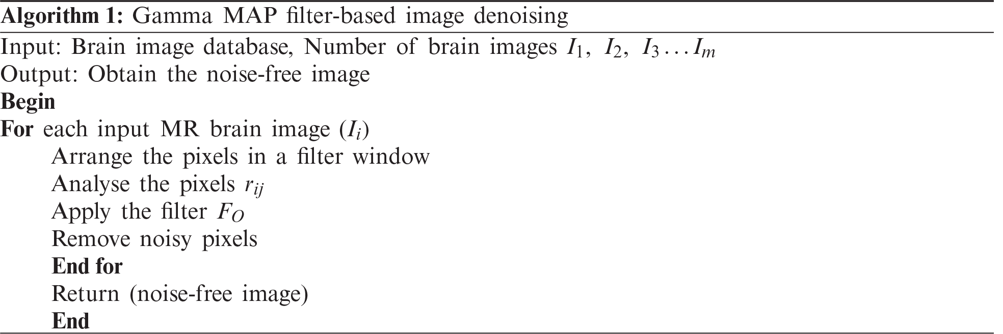
The GMDSWS-MEC model performs image pre-processing for obtaining noise free images by removing the noisy artefacts from the input brain images using the Gamma MAP filter for accurate tumour detection. The Gamma MAP filter is applied for analysing the pixels in the given input MRI images and removing the noisy pixels.

Let us consider the input brain MRI images denoted as I1, I2, I3…Im and the pixels denoted as r1, r2, r3, …rm. The pixels are arranged in a filter window based on the gamma distribution. Fig. 2 illustrates the 3 × 3 filter window in which the image pixels are positioned in terms of rows (i) and columns (j).

As illustrated in Fig. 2, the centre pixel rij is changed with the weighted sum of the neighbourhood pixel value in the filter window. The centre value of the filter window is taken by organising the pixels in ascending order, considering the centre value.

Figure 2: 3 × 3 Matrix format

If the neighbouring pixel values are even, then the average of these two pixels are taken as the centre pixel. The output of the Gamma MAP filter is expressed as follows:

FO=β+d(m−ri), (1)

β=arg maxPr(ri|N), (2)

where FO indicates a filter output, and β denotes a MAP function. The proposed filter uses the prior knowledge of the probability distribution function (Pr), and argmax indicates the argument of the maximum function. The filter finds the maximum probability of the noisy pixels (N), where d represents the local variance, m denotes a local mean within the filter window, and ri denotes the pixels of images. From the analysis, the pixels which are deviated from the local mean value are filtered and replaced by the weighted average (i.e., mean) of all the pixels in the filter window.

2.2 Strömberg Wavelet Transform Segmentation

Once the image pre-processing is completed, the Strömberg wavelet transform segmentation is carried out to segment the pre-processed image into a number of small areas based on the features such as texture, shape, grey level intensity, and colour.

The Strömberg wavelet transform segmentation minimises the time for tumour detection. By applying segmentation, the process of feature extraction for all pixels in the image is avoided, and only the features of interest are extracted. The block diagram of the Strömberg wavelet transform segmentation is demonstrated in Fig. 3. The pre-processed image is decomposed into a number of blocks, and the Strömberg wavelet transform is applied to each block.

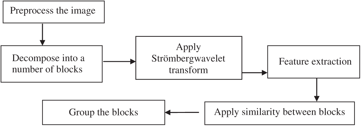
Figure 3: Block diagram of the Strömberg wavelet transform segmentation

The Strömberg wavelet is an orthogonal wavelet transform that decomposes the blocks into a number of sub bands with two different ranges of frequencies, such as low (l) and high (h).

Fig. 4 demonstrates the image decomposition by Strömberg wavelet. In the first level transformation, the input pre-processed image is decomposed into two levels: low (l) and high (h). Wavelet transformation is implemented by using a pair of filters in both horizontal and perpendicular directions of the input image. For the subsequent levels, down sampling (i.e., ↓2) is carried out, and the output of each level generates four sub-blocks ll, lh, hl, hh. A similar procedure is performed again on the sub-block image to generate the next decomposition level. The transformation is applied as given in Eq. (3):

φ(t)=2b/2DC(2bt−v), (3)

where φ(t) indicates the transformation at timet, b and v indicates the integer (v=1, 2, 3, ..), and DC indicates the Strömbergwavelet of order c.

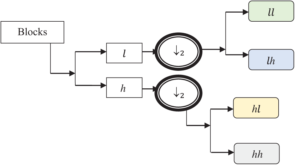
Figure 4: Image decomposition

After decomposition, the features such as texture, shape, grey level intensity, and colour are extracted from each of the sub bands to create a feature vector.

Image texture R provides the knowledge about the spatial display of colour or intensities in the selected block of an image. The texture is measured based on the correlation measure.

R=∑i∑j(ri−μi)(rj−μj)(ri,rj)σiσj, (4)

where R is the texture feature of an image, μi and μj are the respective means of the pixels ri and rj, and σiσj denotes a deviation of the pixels. The shape features are extracted by contours in which the centre of the image is denoted by (0, 0). Then, the distance Dis from the centre to the edge is calculated to determine the shape. Therefore, the distance is measured as Eq. (5):

Dis=(u2−u1)2−(v2−v1)2, (5)

where Dis indicates the distance.The point (u1, v1) represents the centre, i.e., (0, 0), and the point (u2, v2) denotes an edge. In this way, each point on the perfect shape of the boundary is extracted.

The grey level intensity contrast Sb is measured as the difference between the pixel (ri) and its neighbouring pixels (rj) in the set of pixels as given in Eq. (6):

Sb=∑i∑j|ri−rj|2. (6)

The colour features are extracted by transferring the RGB image into HSV (hue, saturation, value) colour spaces as given in Eq. (7):

C=1mIp, (7)

where C indicates the colour feature of the image block, Ip denotes the pixel intensity, and m denotes the total number of pixels in an image.

with the extracted features, the feature vector is created, and the similarity is measured for segmenting the blocks based on the similar features. The dice similarity is calculated using Eq. (8):

ρ=2∗(Fwi∩FwjFwi∪Fj), (8)

where ρ is a dice similarity coefficient, Fwi represents the feature vector of the block wi, and Fwj is the feature vector of the block wj. The intersection symbol ‘∩’ denotes a mutual independence between the feature vectors of the two blocks, and the union symbol ′∪′ represents a mutual dependence. The similarity coefficient (ρ) provides a similarity value in the range from 0 to 1. Likewise, the similarity values of features in all blocks are computed. Based on the similarity values, the blocks are grouped to obtain the segmented regions of the images.

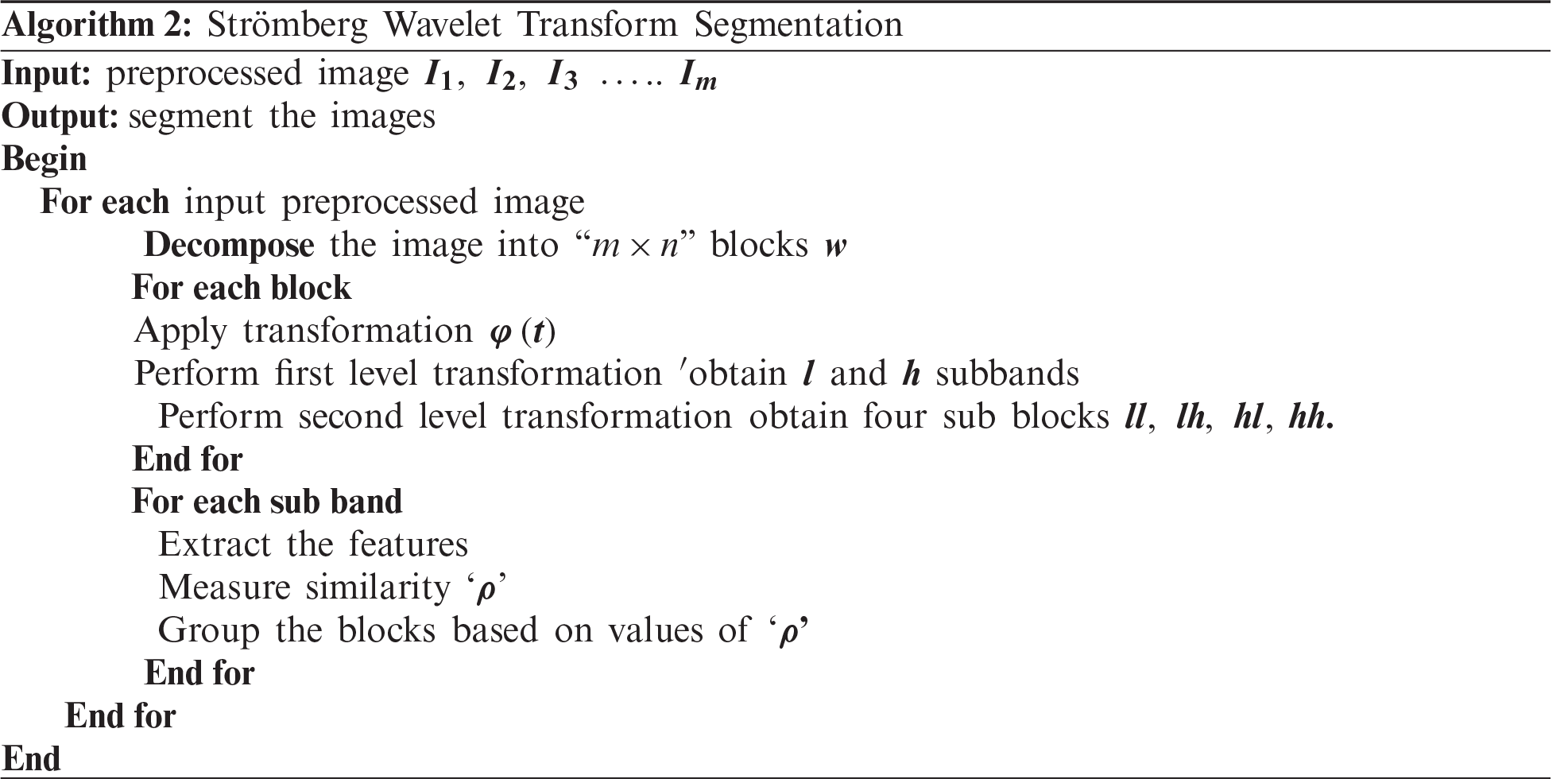
The segmentation process of the proposed method minimises the tumour detection time. The process of the Strömberg wavelet transform segmentation is described in Algorithm 2.

2.3 Maximum Entropy Classifier for Tumour Detection

The final process of the GMDSWS-MEC model is the classification to detect the brain tumour with higher accuracy. The GMDSWS-MEC model uses the maximum entropy classification technique to perform tumour detection with the extracted feature vectors.

The maximum entropy classifier, a machine learning technique and probabilistic classifier, is used to classify the images based on mutually dependent features and detect brain tumours. Fig. 5 depicts the block diagram of the maximum entropy classifier for detecting brain tumours.

The maximum entropy classifier uses the feature vector as the input, and the output of final classification is obtained with Eq. (9):

Y=arg⁡ max[D(x, M|c)], (9)

where Y indicates the output of maximum entropy classifier, arg⁡max denotes an argument of the maximum function, D(x, M|c) is the probabilistic function, which provides the values between 0 and 1, x is the input (i.e., images), c indicates the output classes (normal, tumour), and M denotes the feature matching function. The probability results are obtained based on feature matching, which is expressed as Eq. (10):

M=‖Ev−TEv‖2, (10)

where M is the feature matching function, Ev denotes an extracted feature vector, TEv denotes a disease testing feature vector, and ‖Ev−TEv‖ indicates the distance between the two feature vectors. If the distance is minimum, then the image is classified as a tumour; otherwise, the image is classified as normal. The minimum distance has a maximum probability of tumour occurrence. Therefore, the GMDSWS-MEC model accurately finds tumours in MRI images.

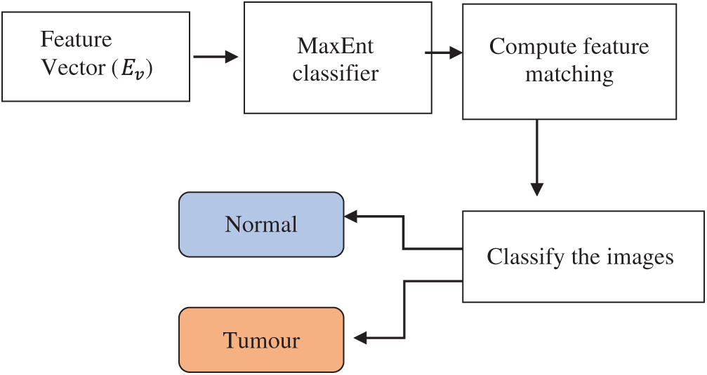
Figure 5: Block diagram of maximum entropy (MaxEnt) classifier

The description of the maximum entropy classifier is explained in Algorithm 3. The above process indicates that the maximum entropy classifier is used for tumour detection. The proposed classifier takes a feature vector as the input, which is matched with the disease features.

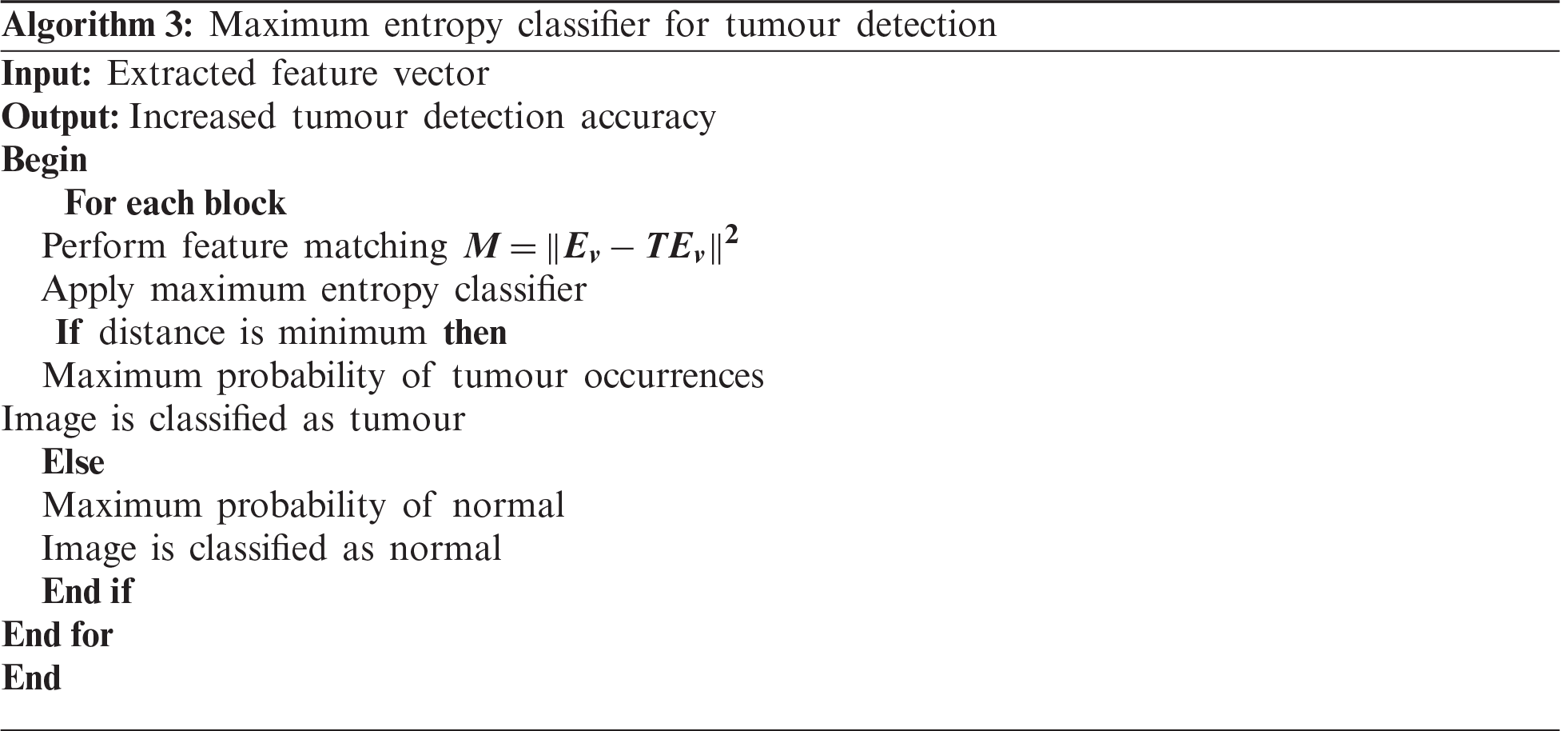
The distance function is used to find the extracted feature most similar to the testing feature. If the two features are correctly matched, then the image has a maximum probability of tumour occurrence. If the two features deviate from each other, then the image is classified as normal. As a result, the proposed classifier accurately finds the tumour with minimal error rate.

3  Experimental Setup

Using MATLAB software, experimental assessment of the proposed GMDSWS-MEC model’s ability to detect brain tumours in MRI images is performed alongside the conventional methods, that is, the PCA-NGIST with RELM classifier proposed by Gumaei et al. [1] and the PNN classifier developed by Shree et al. [2], for comparison.

3.1 Database Description

Brain MRI images of more than 25,500 patients are collected from hospitals and stored in the form of a database https://radiopaedia.org/cases/anaplastic-astrocytoma-8?lang=us. For the experimental assessment, 150 images are considered to perform statistical evaluation with various input parameters.

3.2 Parameter Explanation

To evaluate the performance of the GMDSWS-MEC model and the two conventional methods, PCA-NGIST-RELM and PNN, four quantitative metrics are used. The metrics are described below.

3.2.1 Peak Signal-to-Noise Ratio (RPS)

The peak signal-to-noise ratio is measured as the ratio of the original pixel value to the mean square error. The mean square error is measured as the difference between the size of the original image and the size of the denoised image. Therefore, the peak signal-to-noise ratio RPS and the mean square error rate mser are mathematically computed as

RPS=10∗log10⁡(M2mser), (11)

mser=[Sized−Sizeo]2, (12)

where RPS denotes the peak signal-to-noise ratio, M2 indicates the maximum possible pixel value (255), mser is the mean square error, Sized is the denoised image size, and Sizeo refers to the original image size. The measurement of RPS is obtained in the unit of decibels (dB).

3.2.2 Tumour Detection Accuracy (ACtd)

Tumour detection accuracy is an important metric used to compare the performance of the proposed algorithm against the existing methods. It refers to the ratio of the number of input MRI images that are correctly identified as tumour or normal. The formula to calculate the tumour detection accuracy is given in Eq. (13) as

ACtd=[IcdIn]∗100, (13)

where In indicates the number of images taken as input, and Icd is the number of MRI images correctly detected as tumour.

3.2.3 Error Rate (Rer)

The error rate is the ratio of the number of MRI images mistakenly identified as tumour or normal. The ratio is mathematically computed as

Rer=[ImdIn]∗100, (14)

where In is the number of MRI images taken for experimental evaluation, and Imd is the number of MRI images mistakenly detected. The error rate is expressed in the unit of percentage (%).

3.2.4 Tumour Detection Time (Ttd)

The tumour detection time is the time taken by the algorithm to detect the tumour from the given input MRI images. The time is calculated as

Ttd=In∗t(DSI), (15)

where In is the number of input MRI images, t denotes a time, and DSI is the detected single MRI image. The time for tumour detection is expressed in milliseconds (ms).

4  Performance Analysis

Experiments are conducted with 10 runs for each classification model. The performance of the GMDSWS-MEC model is compared to the state-of-the-art methods with various parameters.

Initially, the peak signal-to-noise ratio is analysed with respect to various sizes of the input MRI images taken from the database. The reported results shown in Tab. 1 reveal that the peak signal-to-noise ratio is higher and the mean square error rate is lower using the proposed method. As illustrated in Tab. 1, the input is considered as the sizes of the various MRI images

The results of the three methods are illustrated in Fig. 6. Overall, the average peak signal-to-noise ratio of the GMDSWS-MEC model is 6% and 10% better than that of the PCA-NGIST with RELM and PNN, respectively.

The reason for the improvement in peak signal-to-noise ratio with the GMDSWS-MEC model is the use of the Gamma MAP filter for pre-processing. The proposed filter is applied to remove the noisy artefacts from the input MRI images in the filter window. Therefore, the filter provides images of enhanced quality.

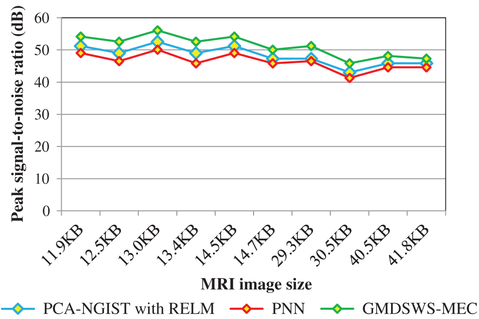
Figure 6: Graphical illustration of the peak signal-to-noise ratio

The second metric used for comparison is the tumour detection accuracy, which helps to analyse the efficiency of the proposed algorithm in detecting tumours from MRI brain images. In this scenario, the numbers of input images is considered as the input to all three methods. The input image counts for the various methods that range from 15 to 150.

Tab. 2 reports the performance results of tumour detection accuracy and error rate of the three methods. Ten results are analysed for each method, with similar counts of input. The accuracy of the GMDSWS-MEC model is high, and the error rate is minimal. As shown in Tab. 2, with the input of 15 MRI images, the GMDSWS-MEC model accurately classifies 12 images with an accuracy of 80% and an error rate of 20%. In contrast, the other two approaches classify 11 and 10 images, and the accuracies are 73% and 67%, respectively.

Next, the third metric, the error rate, is considered. The error rates of the PCA-NGIS with RELM and PNN are 27% and 33%. From the statistical analysis, the GMDSWS-MEC model outperforms the other two methods.

The higher accuracy of the GMDSWS-MEC model is a result of applying the maximum entropy classifier. The classifier provides probabilistic results by matching feature vectors. The features extracted from the input MRI images are matched with the testing disease features. If the matching is perfectly done, then the classifier effectively finds the tumour with maximum probability or classifies the image as normal. Additionally, the Gamma MAP filter is applied to obtain the noise-free image.

Therefore, the GMDSWS-MEC model performs tumour detection with enhanced-quality images, which further results in improved tumour detection accuracy and minimises the error rate.

The experimental results are compared for identifying the performance of the three classification methods. The evaluation results indicate that the accuracy of the GMDSWS-MEC model is 5% greater than PCA-NGIS with RELM and 10% greater than PNN. Moreover, based on the error rate, the GMDSWS-MEC model efficiently reduces the incorrect identification of tumour or normal images. The validation result proves that the error rate is minimised by 30% and 44% compared to the PCA-NGIS with RELM and PNN, respectively. Fig. 7 depicts the tumour detection accuracy achieved with various numbers of MRI images. The accuracy results of the three methods are represented by three different colours. The green curve is the tumour detection accuracy of the GMDSWS-MEC model, which provides the best performance.

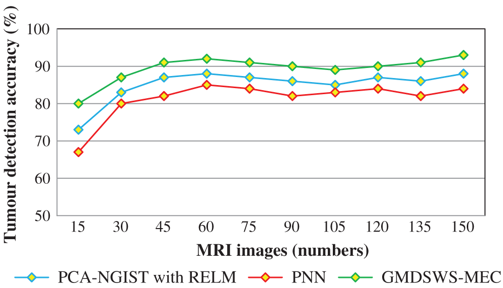
Figure 7: Graphical illustration of the tumour detection accuracy

The comparative analysis of error rate vs. number of MRI images is shown in Fig. 8. The curve indicates that the error rate of the GMDSWS-MEC model is minimised compared to PCA-NGIST with RELM and PNN.

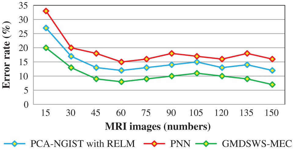
Figure 8: Graphical illustration of the error rate

Finally, the fourth metric, the tumour detection time, is considered. Tab. 3 and Fig. 9 depict the experimental results of tumour detection time of the three methods. As shown in Fig. 9, the time taken to perform the tumour detection increases as the number of images increases. This shows that the tumour detection time is directly proportional to the number of MRI images.

The tumour detection time is found to be minimised using the GMDSWS-MEC model compared to the existing methods. More specifically, the tumour detection time of the GMDSWS-MEC model is 8% less than that of PCA-NGIST with RELM and 13% less than that of PNN. This is due to the application of the Strömberg wavelet transform segmentation method to segment the input image into a number of blocks. For each sub-band, the texture, grey level intensity, shape, and colours are extracted. With the help of extracted features, the input images are classified as normal or tumour. This helps to minimise the time for tumour detection with MRI images.

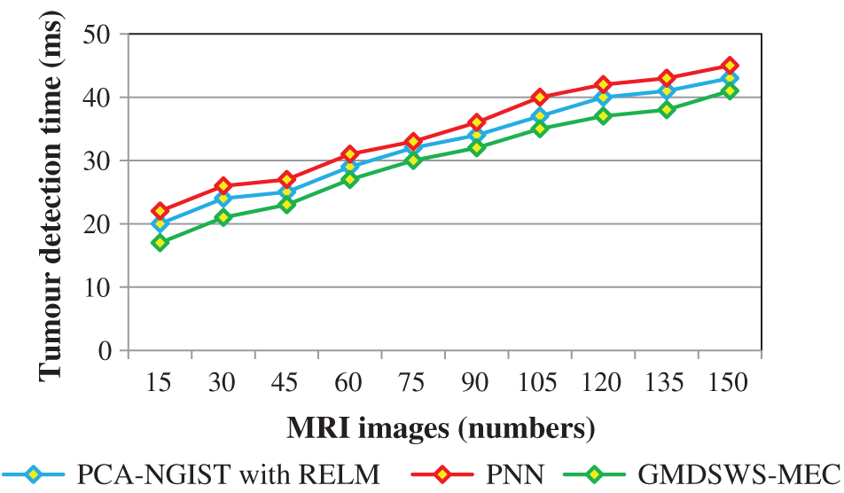
Figure 9: Graphical illustration of the tumour detection time

5  Conclusion

Efficient brain tumour detection plays a vital role in the healthcare industry. The proposed GMDSWS-MEC model employs Strömberg wavelet transformation for segmentation of brain MRI scans and Gamma MAP filter for noise removal. Segmentation is carried out to group different blocks of images based on similar feature vectors. The segmentation process of the GMDSWS-MEC model reduces the amount of time taken for tumour detection. Finally, the probabilistic classifier provides the tumour detection results by matching the feature vectors. The significant matching of features with the GMDSWS-MEC model is unique among the other techniques. Experimental analysis comparing various metrics of the GMDSWS-MEC model with two state-of-the-art methods, namely PCA-NGIST with RELM and PNN, is conducted with numerous MRI images. The results demonstrate that the GMDSWS-MEC model provides satisfactory performance in tumour detection with higher accuracy and minimal time compared to the other two methods.

Funding Statement: The authors received no specific funding for this study.

Conflicts of Interest: The authors declare that they have no conflicts of interest to report regarding the present study.

References

 1.  A. Gumaei, M. M. Hassan, R. Hassan, A. H. Alelaiwi and G. C. Fortino, “A hybrid feature extraction method with regularized extreme learning machine for brain tumor classification,” IEEE Access, vol. 7, pp. 36266–36273, 2019. [Google Scholar]

 2.  N. V. Shree and T. N. R. Kumar, “Identification and classification of brain tumor MRI images with feature extraction using DWT and probabilistic neural network,” Brain Informatics, vol. 5, pp. 23–30, 2018. [Google Scholar]

 3.  Z. Tang, S. Ahmad, P. T. Yap and D. G. Shen, “Multi-atlas segmentation of MR tumor brain images using low-rank based image recovery,” IEEE Transactions on Medical Imaging, vol. 37, no. 10, pp. 2224–2235, 2018. [Google Scholar]

 4.  S. Roy, D. N. Bhattacharyya, S. K. Bandyopadhyay and T. H. Kim, “Heterogeneity of human brain tumor with lesion identification, localization, and analysis from MRI,” Informatics in Medicine Unlocked, vol. 13, pp. 139–150, 2018. [Google Scholar]

 5.  J. Amin, M. Sharif, M. Yasminand and S. L. Fernandez, “A distinctive approach in brain tumor detection and classification using MRI,” Pattern Recognition Letters, vol. 139, pp. 118–127, 2020. [Google Scholar]

 6.  N. B. k. Bahadure, A. K. Ray and H. P. Thethi, “Image analysis for MRI based brain tumor detection and feature extraction using biologically inspired BWT and SVM,” International Journal of Biomedical Imaging, vol. 2017, no. 1, pp. 1–12, 2017. [Google Scholar]

 7.  M. M. Thaha, K. P. M. Kumar, B. S. Murugan, S. Dhanasekeran, P. Vijayakarthick et al., “Brain tumor segmentation using convolutional neural networks in MRI images,” Journal of Medical Systems, vol. 43, no. 294, pp. 1–10, 2019. [Google Scholar]

 8.  M. Sharif, J. Amin, M. Raza, M. A. Anjum, H. Afzal et al., “Brain tumor detection based on extreme learning,” Neural Computing and Applications, vol. 32, pp. 15975–15987, 2020. [Google Scholar]

 9.  A. Edalati-rad and M. Mosleh, “Improving brain tumor diagnosis using MRI segmentation based on collaboration of beta mixture model and learning automata,” Arabian Journal for Science and Engineering, vol. 44, pp. 2945–2957, 2019. [Google Scholar]

10. F. Özyurt, E. Sert and D. Avcı, “An expert system for brain tumor detection: Fuzzy C-means with super resolution and convolutional neural network with extreme learning machine,” Medical Hypotheses, vol. 134, pp. 1–8, 2020. [Google Scholar]

11. R. Rajagopal, “Glioma brain tumor detection and segmentation using weighting random forest classifier with optimized ant colony features,” International Journal of Imaging System and Technology, vol. 29, no. 7, pp. 1–7, 2019. [Google Scholar]

12. J. Amina, M. Sharif, M. Razaa, T. Z. Saba and M. A. Anjum, “Brain tumor detection using statistical and machine learning method,” Computer Methods and Programs in Biomedicine, vol. 177, no. 3, pp. 69–79, 2019. [Google Scholar]

13. A. R. Abdulraqeb, W. A. Al-Haidri, L. T. Sushkova, M. M. Abounassif, P. J. Parameaswari et al., “An automated method for segmenting brain tumors on MRI images,” Biomedical Engineering, vol. 51, no. 2, pp. 97–101, 2017. [Google Scholar]

14. M. Nasor and W. Obaid, “Detection and localization of early-stage multiple brain tumors using a hybrid technique of patch-based processing, k-means clustering and object counting,” International Journal of Biomedical Imaging, vol. 2020, no. 2, pp. 1–9, 2020. [Google Scholar]

15. F. Özyurt, E. Sert, E. Avci and E. Dogantekin, “Brain tumor detection based on convolutional neural network with neutrosophic expert maximum fuzzy sure entropy,” Measurement, vol. 147, pp. 1–7, 2019. [Google Scholar]

16. A. Bal, M. Banerjee, A. Chakrabarti and P. Sharma, “MRI brain tumor segmentation and analysis using rough-fuzzy C-means and shape based properties,” Journal of King Saud University-Computer and Information Sciences, vol. 32, pp. 1218–1237, 2018. [Google Scholar]

17. S. M. K. Hasan and M. Ahmad, “Two-step verification of brain tumor segmentation using watershed-matching algorithm,” Brain Informatics, vol. 5, no. 8, pp. 1–11, 2018. [Google Scholar]

18. G. S.Manogaran, P. M. Shakeel, A. S. Hassanein, P. M. V. Kumarand and G. N. C. Babu, “Machine learning approach-based gamma distribution for brain tumor detection and data sample imbalance analysis,” IEEE Access, vol. 7, pp. 12–19, 2018. [Google Scholar]

19. R. B. Vallabhaneni and V. Rajesh, “Brain tumour detection using mean shift clustering and GLCM features with edge adaptive total variation denoising technique,” Alexandria Engineering Journal, vol. 57, no. 4, pp. 2387–2392, 2018. [Google Scholar]

20. P. R. Lorenzo, J. Nalepaa, B. Bobek-Billewicz, P. Wawrzyniak and G. G. Mrukwa, “Segmenting brain tumors from FLAIR MRI using fully convolutional neural networks,” Computer Methods and Programs in Biomedicine, vol. 176, pp. 135–148, 2019. [Google Scholar]

21. T. Maekawa, M. Hori, Katsutoshi Murata, Thorsten Feiweierand and K. Kamiya, “Differentiation of high-grade and low-grade intra-axial brain tumors by time-dependent diffusion MRI,” Imaging Magnetic Resonance Imaging, vol. 72, pp. 34–41, 2020. [Google Scholar]

22. K. S. A. Viji and D. H. Rajesh, “An efficient technique to segment the tumor and abnormality detection in the brain MRI images using KNN classifier,” Biomedical Signal Processing and Control, vol. 24, no. 3, pp. 1944–1954, 2020. [Google Scholar]

23. J. Zhaoa, D. W. Li, Z. Kassam, J. Howey and J. Chongc, “Tripartite-GAN: Synthesizing liver contrast-enhanced MRI to improve tumor detection,” Medical Image Analysis, vol. 63, pp. 101667, 2020. [Google Scholar]

This work is licensed under a Creative Commons Attribution 4.0 International License, which permits unrestricted use, distribution, and reproduction in any medium, provided the original work is properly cited.