DOI:10.32604/cmc.2021.017995
| Computers, Materials & Continua DOI:10.32604/cmc.2021.017995 | |
| Article |
Optimal Implementation of Photovoltaic and Battery Energy Storage in Distribution Networks
1Department of Electrical Engineering, Faculty of Engineering, Aswan University, 81542 Aswan, Egypt
2College of Engineering at Wadi Addawaser, Prince Sattam Bin Abdulaziz University, 11911 Al-Kharj, Saudi Arabia
3Electrical Engineering Department, Faculty of Engineering, Minia University, 61517 Minia, Egypt
4Department of Electrical Engineering, Yeungnam University, Gyeongsan, 38541, Korea
*Corresponding Author: Sang-Bong Rhee. Email: rrsd@yu.ac.kr
Received: 20 February 2021; Accepted: 4 March 2021
Abstract: Recently, implementation of Battery Energy Storage (BES) with photovoltaic (PV) array in distribution networks is becoming very popular in overall the world. Integrating PV alone in distribution networks generates variable output power during 24-hours as it depends on variable natural source. PV can be able to generate constant output power during 24-hours by installing BES with it. Therefore, this paper presents a new application of a recent metaheuristic algorithm, called Slime Mould Algorithm (SMA), to determine the best size, and location of photovoltaic alone or with battery energy storage in the radial distribution system (RDS). This algorithm is modeled from the behavior of SMA in nature. During the optimization process, the total active power loss during 24-hours is used as an objective function considering the equality and inequality constraints. In addition, the presented function is based on the probabilistic for PV output and different types of system load. The candidate buses for integrating PV and BES in the distribution network are determined by the real power loss sensitivity factor (PLSF). IEEE 69-bus RDS with different types of loads is used as a test system. The effectiveness of SMA is validated by comparing its results with those obtained by other well-known optimization algorithms.
Keywords: Slime mould algorithm; optimization; distribution networks; renewable energy; uncertainty
Most of electrical energy around the world are coming from fossil fuel to meet the required electrical demand [1]. The utilization of fossil fuels harms the environment and lead to global warming and air pollution. Also, the electrical loads are increasing gradually due to world population growth and technology development that led to increasing in system power losses. These losses are occurred with percent 70% in the secondary and primary distribution system and with percent 30% in sub transmission and transmission lines [2]. Therefore, integrating renewable sources (RSs) in distribution networks is the best solution for decreasing the system power loss and support power to the load with clean and sustainable energy compared to fossil fuel [3]. Most types of RSs that are used in power system are hydropower, biomass, photovoltaic (PV) and wind turbine [4].
PV converts solar energy into electrical energy in a silent way, so installing PV in distribution system has increased around the world [3]. PV alone is non-dispatchable source as PV output depends on variable source (sun) [5,6]. Therefore, BES should be inserted with PV to convert PV into dispatchable source [7]. As long as PV output is low or zero during 24-hours, BES is capable of supplying active power to the system [8]. Therefore, installing PV with BES in RDS decreases the system losses, increases the system capacity, and improves the system voltage. The best locations (buses) up to fifty percent of system buses for integration PV with BES in RDS are obtained using RLSF. The presented problem formulation is the real losses of the system as single objective function.
SMA can be classified as one of recent metaheuristic algorithms that is created from the behaviors of slime moulds in nature [9]. In SMA, there are weights are used to model the negative and positive feedback of slime mould when searching for food. SMA has an efficient exploration and exploitation phases to determine the best solution with minimum search agent. SMA has a feedback behavior which enhances the characteristic of SMA to avoid the local solutions and go to the global results so far. SMA is used to obtain the optimal allocation of PV with BES in RDS. Metaheuristic algorithms are more popular because of their effectively in solving difficult problems. Many types of metaheuristic algorithms are applied to determine the optimal planning of PV with BES in RDS such as Genetic algorithm (GA) which is used to determine the sizing of BES with sizeable PV in RDS to minimize the system power loss [10], Linear programming (LP) is used to determine the energy storage dispatch for PV with BES connected in a grid [11], whale optimization algorithm (WOA) for optimal planning of BES in RDS for loss reduction has been presented in [12], grey wolf optimizer algorithm (GWO) for optimal allocation of BES in RDS to minimize the total annual cost of the system has been presented in [13], Artificial Bee Colony (ABC) for optimal placement and sizing of PV and electric vehicle in RDS for loss minimization has been presented in [14].
The main contributions of this work can be summarized in the following points:
– A new application of a recent metaheuristic algorithm called Slime Mould Algorithm (SMA) is proposed to determine the best locations and sizes of PV and BES, considering the probabilistic of PV generation and different types of system load.
– The optimal allocations of PV and BES are obtained with the aim of achieving the maximum reduction in the total active power losses.
– The obtained results show that integration of PV and BES in RDS reduces the system power loss, enhances the system voltage, and increases the system capacity.
– The simulation results also prove that integration of PV with BES gives better results than integration of PV alone in RDS.
This paper can be divided into subsection as follows: The presented problem can be formulated in Section 2, modeling of load and PV with BES is offered in Section 3, the sensitivity is discussed in Section 4, Section 5 presents the presented algorithm, Section 6 discusses the obtained results, and Section 7 presents the conclusion.
Fig. 1 represents a section of two nodes in RDS.
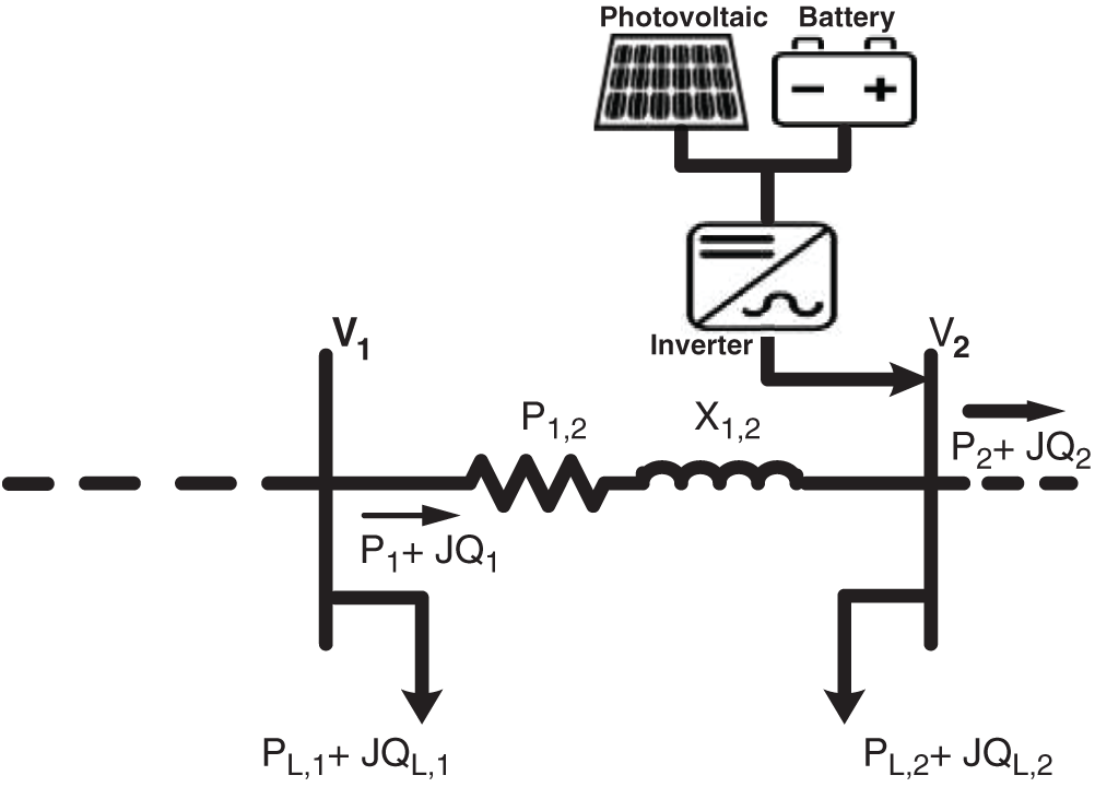
Figure 1: Representation of two buses in main feeder with PV and BES
Forward-backward sweep algorithm is presented to calculate the power flows of RDS [15]. In backward direction, the reactive and real power can be obtained as follows:
where, Pu and Pu+1 represent the active power behind bus (u) and bus (u+1), respectively. Xu, u+1 and Ru, u+1 represent the reactance and resistance of the branch among bus (u) and bus (u+1), respectively. Qu and Qu+1 are the reactive power behind bus (u) and (u+1), respectively. QL, u+1 and PL, u+1 represent the reactive and active loads at bus (u+1), respectively.
In forward direction, the voltage magnitude of bus (u+1) is obtained as follows:
here, Vu and Vu+1 represent the voltage values at bus (u) and bus (u+1), respectively.
System power flows will be changed as PV with BES will inject active power to the distribution system. Consequently, system power flow equations is updated as shown in Eqs. (4) and (5).
The presenting mathematical problem is defined as shown in Eq. (6).
where, PLoss(t) is the total active power loss at time (t).
This function is presented under equality and inequality constraints as shown next [16].
The power supplied by substation and PV with BES must be equal to the system loss and system load demand as follows:
where, Po and PL are the active power injection from substation and active load demand, respectively. Qo and QL are reactive power injection from substation and reactive load demand, respectively. PPV+BES is the power supplying by PV and BES and QLoss is the reactive loss of the system. NB and NBr are the total number of buses and branches in RDS, respectively. N is the total number PV with BES in RDS.
The bus voltage in RDS should be kept between the low and high operating voltage, as given in Eq. (9).
where, VB is the voltage magnitude of bus B that should be obtained between minimum value of VD and maximum value of VU
2.2.2 PV with BES Sizing Limits
The sizing limits of PV and BES are given as follows:
where, PPV, U and PPV, D represent the maximum and minimum magnitudes of PV output power, respectively. EBES, U and EBES, D represent the upper and lower magnitudes of energy stored in BES.
Lines current should not exceed the limit values [17].
where, IW and
3 Modeling Uncertainty for Load and PV with BES
3.1 Modeling Uncertainty for Load
The uncertainties of system loads can be modeled as different load patterns (residential, industrial and commercial loads) during 24-hours daily, as shown in Fig. 2 [18]. This model is based on a time-varying during 24-hours and voltage-dependent load [19]. Therefore, the system load modeling can be represented by Eqs. (14) and (15).
where, QB and PB represent the reactive and active power injections at bus (B), QL, B and PL, B represent the reactive and active loads at bus (B), nac is the active load voltage exponent that equal to 0.18, 1.51 and 0.92 for industrial, commercial and residential load modeling, respectively [19].
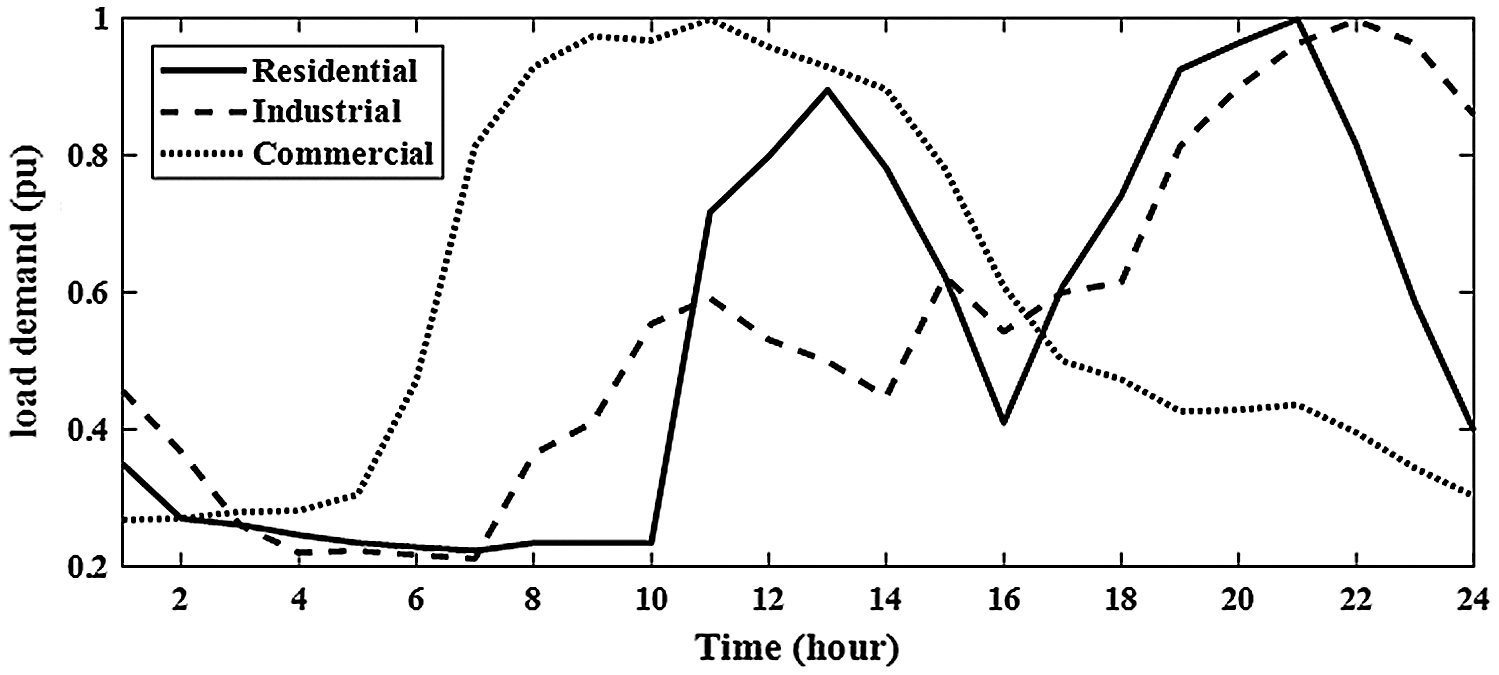
Figure 2: Modeling uncertainty for system loads during 24-hours daily
3.2 Modeling Uncertainty for PV Output
PV generates electricity from solar irradiance during 24-hours. From Fig. 3, the modeling uncertainty for PV output is created by PDF [20]. The standard deviation and mean of solar radiation are given by [21].
where, FB(r) represents the the function of Beta distribution for solar radiation (r).
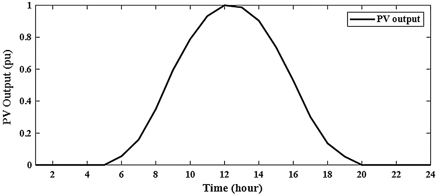
Figure 3: Modeling uncertainty for PV output during 24-hours daily
The output of PV depends on the solar irradiance and air temperature, so the specification of PV panel are given by [21]. The maximum power of PV can be determined by Eq. (18).
where, Kvo and Kcu are the voltage and current temperature coefficient in voltage per Celsius and ampere per Celsius, respectively. Tamb and Tcell are the air and cell temperature in Celsius, respectively. n and no are the total number of PV modules and the nominal temperature of cell in Celsius, respectively. Isc and Vop and are the short circuit current and the open-circuit voltage, respectively.
3.3 Battery Energy Storage Modeling
PV alone can be considered as non-dispatchable source, so BES is installed with PV to convert PV into a dispatchable source. BES is charged when PV output is more than the required output power and is discharged when PV output is zero during night or less than the required output power. The energy that is stored in BES at bus (B) during 24-hours can be determined by Eqs. (23) and (24) [20].
where,
The locations and sizes of PV with BES are obtained by the presented algorithm. The installation bus of BES is identical to the bus of PV. The discharging/charging energies of BES during a time (h) is determined by Eqs. (26) and (27) [21].
The combined energy of PV with BES E(PV+BES), u and the energy of PV EPV, u at bus (u) can be evaluated as follows:
where,
Consequently, Eq. (29) can be updated as follows:
where, n represents the PV module unit.
The high value of PV can be evaluated by Eq. (34).
where,
The BES energy is determined by Eq. (35).
4 Real Power Loss Sensitivity Factor (PLSF)
PLSF measures the sensitivity of all system buses to the active power injection and its effects on the active power loss. Therefore, this paper determines the best buses for installing PV with BES up to 50% of system buses by Eq. (36) [22]. The best bus are 57, 58, 7, 6, 61, 60, 10, 59, 55, 56, 12, 13, 14, 54, 15, 53, 8, 64, 49, 11, 9, 17, 65, 16, 5, 48, 21, 19, 41, 63, 68, 34, 20 and 62 as shown in Fig. 4.
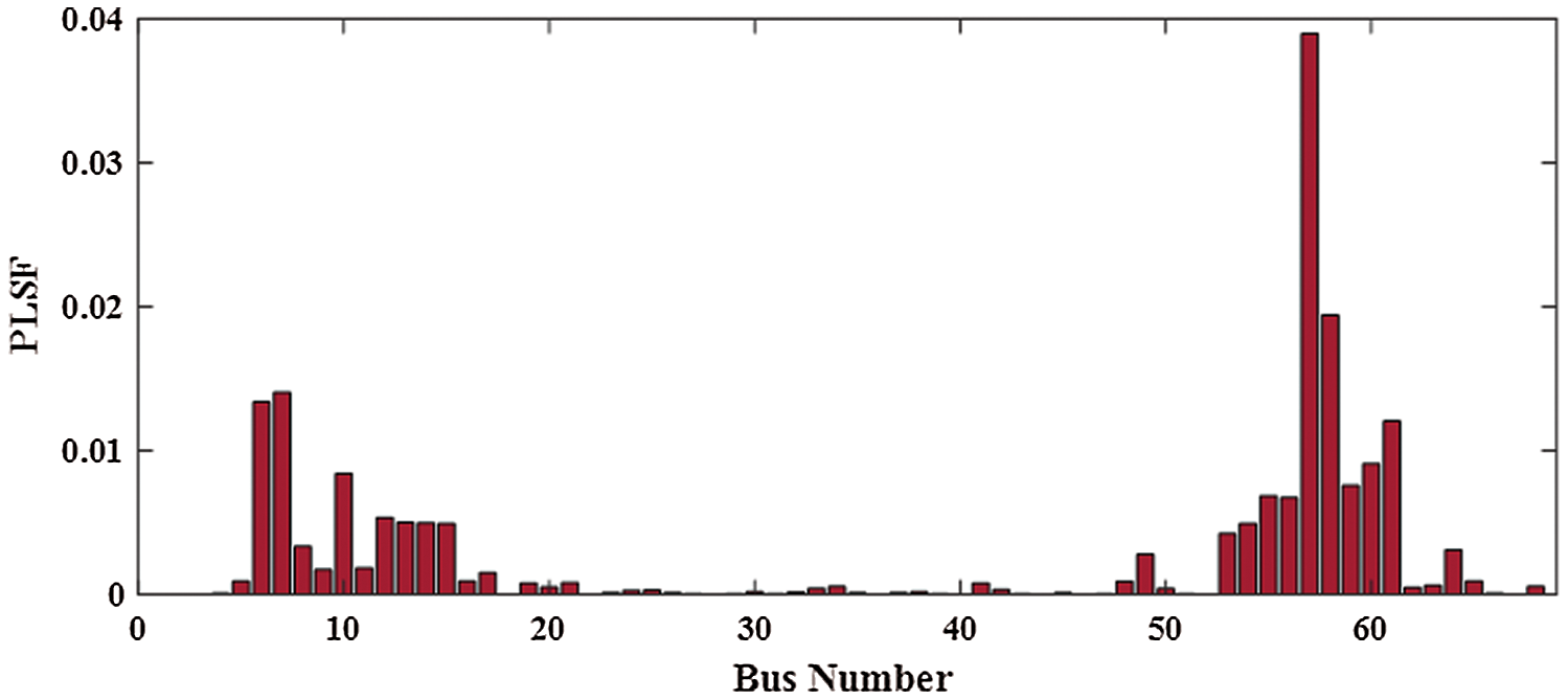
Figure 4: PLSF for IEEE 69-bus RDS
SMA can be classified as one of recent metaheuristic algorithms that is created from the behaviors of slime moulds in nature [9]. Slime mould searches for quality food through the odor in the air. The behavior mechanism of slime mould is based on contraction mode. Slime mould consists of venous tissues and the width of vein will be increased as long as this vein is closer to the higher concentration of quality food. When a vein reaches to the higher concentration of food, the biological oscillator generates waves to change the cytoplasmic flow to this vein and its width will be increased. The steps of SMA for determining the best position and size of PV with BES considering uncertainty in RDS is explained in the following steps.
Step 1 : Read system data, number of search agents (N) and maximum iteration (T).
Step 2 : Generate initial population of slime mould between the lower (lo) and upper (up) controlled variables by Eq. (37).
where, Q is the number of control variables (dimensions) and r and represents a random value between value of 0 and 1.
Step 3 : the produced population represents the slime mould position that can be formulated as follows:
where, J is the position of slime mould.
Step 4 : Evaluate the fitness for all locations of slime mould in all swarms and obtain the best and worst fitness and the best position of slime mould.
Step 5 : Calculate the weight (w) of each position of slime mould as follows:
where, S(i) is the fitness each position of slime mould for search agents and condition refer to that S(i) ranks first half of search agents
Step 6 : Update the position of slime mould as follows:
where JA and JB are the position of slime mould that are selected randomly from the search agents. DF is the best fitness and z is a parameter that equal to 0.03. e and E represent the current iteration and the final iteration, respectively vb represents a value which oscillates between (-a) and (a) and reaches to zero at the maximum iteration. vc is a value that oscillates between ( −1) and (1) and reaches to zero at the maximum iteration.
Step 7 : Back to step 4 until the final iteration is reached.
Step 8 : Obtain the best location of slime mould (sizes and positions of PV alone or with BES).
IEEE 69-bus RDS consists of sixty nine buses with reactive load of 2694.6 kvar and active load of 3801.5 kw as shown in Fig. 5 [23]. In this paper, the simulation results are obtained under base values of 10 MVA and 12.66 kv. The system constraints and the used parameter algorithm are given in Tab. 1.
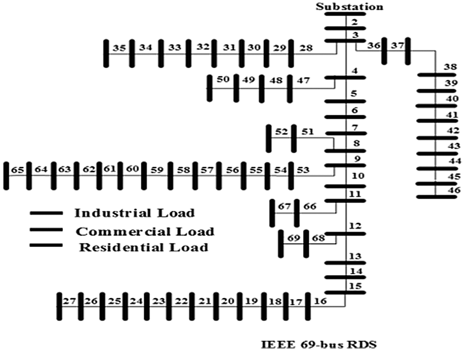
Figure 5: IEEE 69-bus RDS with different load types

Without integration PV alone or with BES in RDS, the power loss is 1867.8 kw with minimum voltage of 0.9110 pu at bus 65 during 24-hours as shown in Fig. 6. The system power loss is reduced to 1521.2 kw by integrating one PV in RDS with size of 1288.164 kw at bus 61 as shown in Fig. 7. From Fig. 8, the system power loss is reduced to 1481.7 kw by integrating two PV alone in RDS with sizes of 1216.7 kw at bus 61 and 416.3 kw at bus 17. From Fig. 9, integrating three PV alone reduces the system power loss to 1474.5 kw with sizes of 1168.9 kw, 302.2 kw and 398.5 kw at buses 61, 17 and 11, respectively. From obtained results, the reduction in real power loss by installing one, two and three PV alone in RDS are 18.6%, 20.7% and 21.1%, respectively. From Tab. 2, the total injection energies from one, two and three PV to the system are 9695.3 kwh, 12290.9 kwh and 14070.8 kwh, respectively. Installing PV with BES achieves better results than integrating PV alone in RDS as shown in Tabs. 2 and Tab. 3. Integrating one, two and three PV with BES minimize the system losses to 712.025 kw, 615.13 kw and 596.661 kw, respectively. From obtained results, the reduction in real power loss by installing one, two and three PVwith BES in RDS are 61.9%, 67.1% and 68.1%, respectively. From Figs. 10 and 11, the sizes of PV and BES for installing one PV with BES in RDS are 3797.574 kw and 2772.178 kw at bus 61, respectively. From Tab. 3, integrating one PV with BES, the total energy of PV is 28582.25 kwh and the total injection energy from PV to the grid is 10780.55 kwh. Also, the charging and discharging energies of BES by integrating one PV with BES in RDS are 17801.71 kwh and 13676.68 kwh, respectively.
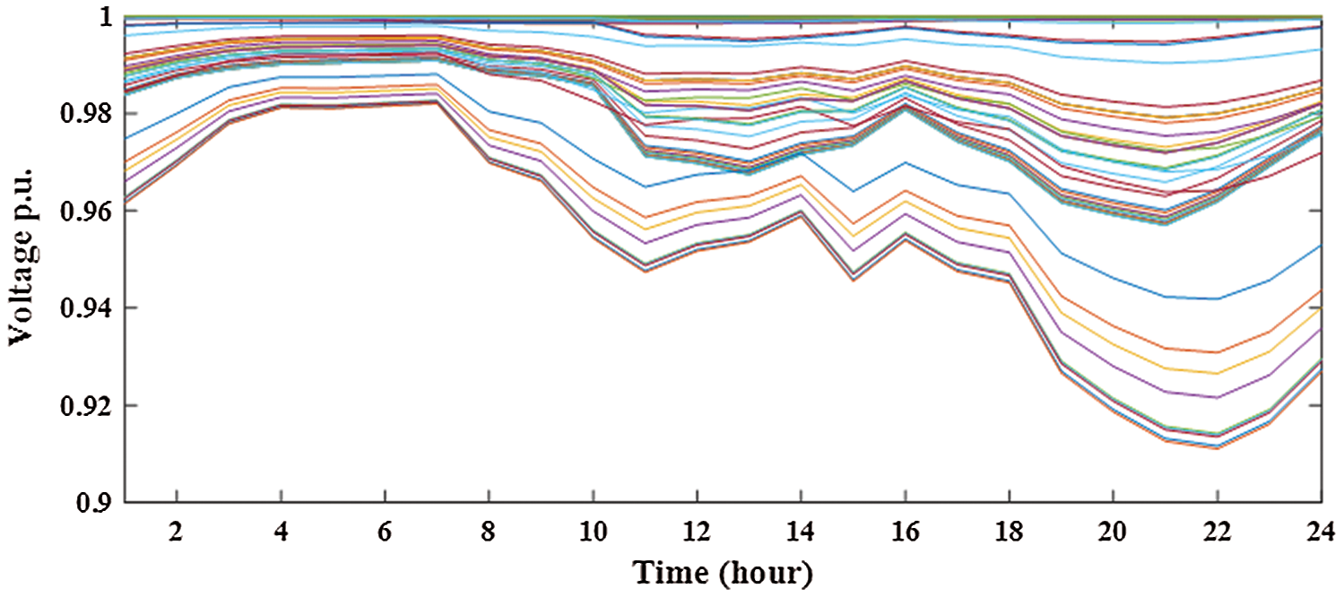
Figure 6: System voltage without integrating PV and BES in distribution network
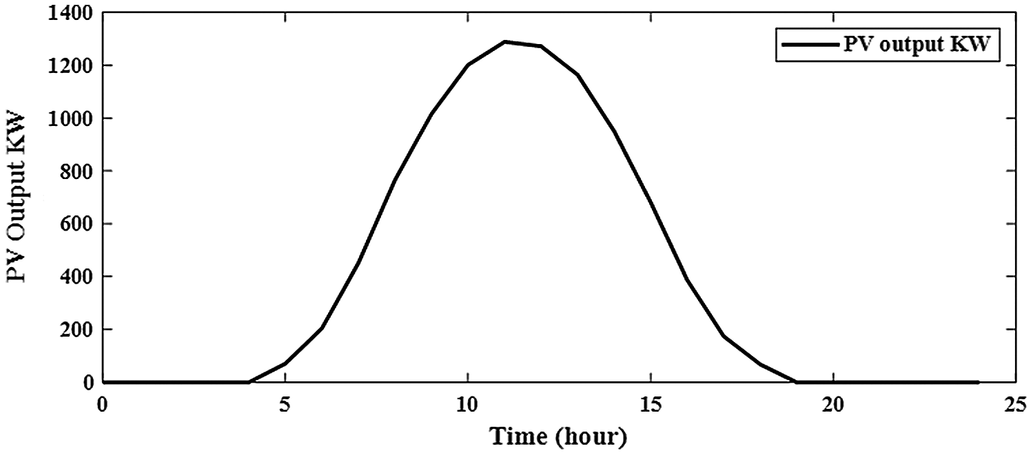
Figure 7: Output of integrating 1-PV alone in distribution network
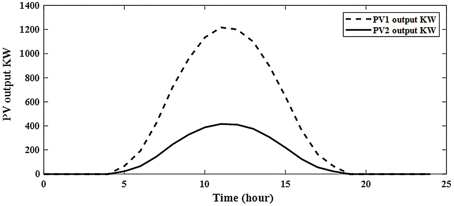
Figure 8: Output of integrating 2-PV alone in distribution network
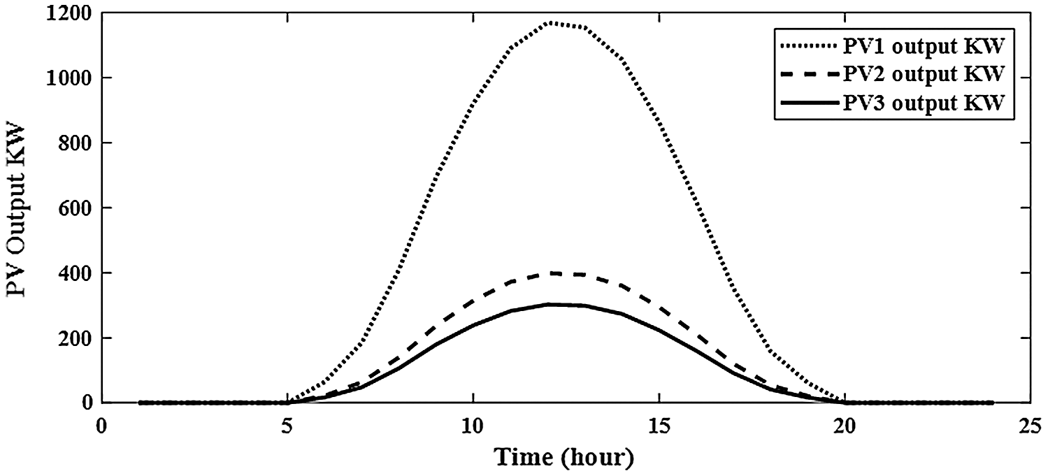
Figure 9: Output of integrating 3-PV alone in distribution network


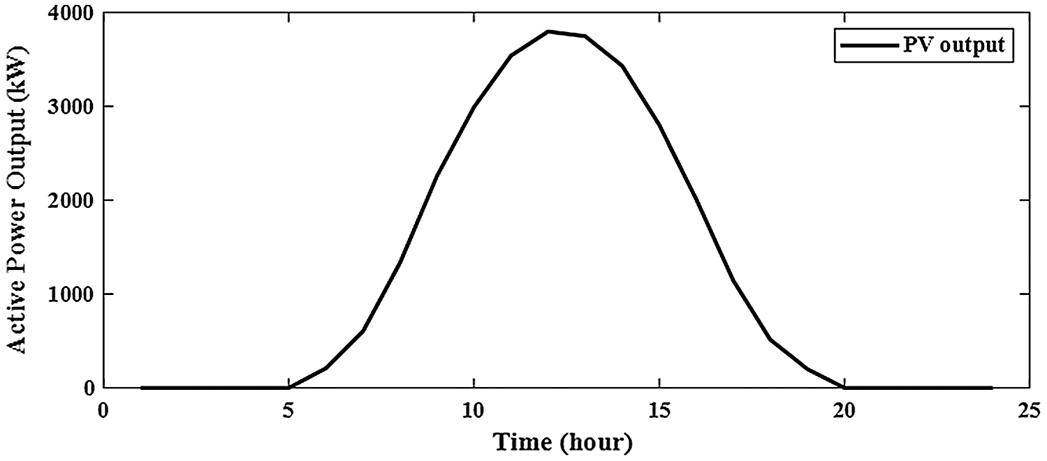
Figure 10: Output of PV for integrating 1-PV with 1-BES in distribution network

Figure 11: Output of BES for integrating 1-PV with 1-BES in distribution network
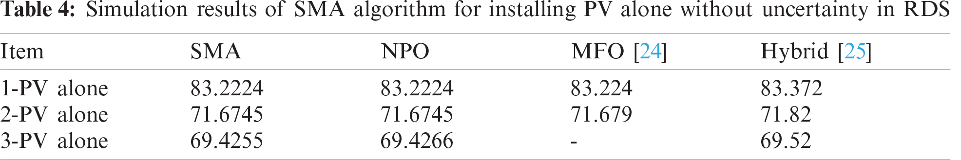
From Fig. 12, the sizes of PV for two PV with BES are 3620.606 kw and 1037.043 kw at buses of 61 and 17, respectively. From Figs. 13 and 14, the sizes of BES for two PV with BES are 2667.004 kw and 690.4277 kw at buses of 61 and 17, respectively. From Tab. 3, the charging energies of BES for two PV with BES are17021.39 kwh and 4535.169 kwh at buses 61 and 17, respectively. The discharging energies of BES for two PV with BES are13077.18 kwh and 3474.439 kwh at buses 61 and 17, respectively. The energies of PV by installing two PV with BES are 27059.54 kw and 7805.258 kw and the injection energies from PV to the grid are 10038.15 kw and 3270.089 kw at buses of 61 and 17, respectively. From Fig. 15, the sizes of PV for three PV with BES are 3499.238 kw, 745.5597 kw and 1016.864 kw at buses 61, 17 and 11, respectively. From Figs. 16–18, the sizes of BES for three PV with BES are 2602.622 kw, 499.0399 kw and 668.2362 kw at buses 61, 17 and 11, respectively. By installing three PV with BES, the energies of PV are 26336.85 kwh, 5611.419 kwh and 7653.377 kwh at buses 61, 17 and 11, respectively. Also, the injection energies from PV to the grid for three PV with BES are 9852.457 kwh, 2361.514 kwh and 3171.519 kwh at buses 61, 17 and 11, respectively. The charging energies of BES for three PV with BES are 16484.39 kw, 3249.905 kw and 4481.858 kw at buses 61, 17 and 11, respectively. From Tab. 3, the discharging energies of BES for three PV with BES are 12664.61 kw, 2489.786 kw and 3433.598 kw at buses 61, 17 and 11, respectively. The size and energy of a combination of PV and BES are greater than the size and energy of PV alone as shown in Tabs. 2 and 3. In this paper, the comparative study is presented to determine the effectivness of SMA to minimize the system losses as objective function without uncertainty. From Tab. 4, SMA is able to obtain the best results compared with other algorithms. Without uncertainty, integration of one, two and three PV alone in RDS reduces the system losses to 83.2224 kw, 71.6745 kw and 69,4255 kw, respectively. The size of one PV is 1872.7 kw at bus 61 and the sizes of two PV are 1781.6 kw at bus 61 and 531.6 kw at bus 17. From Tab. 4, the best result is obtained by integrating three PV with sizes of 1718.9 kw at bus 61, 527.1 kw at bus 11 and 380.5 kw at bus 18.
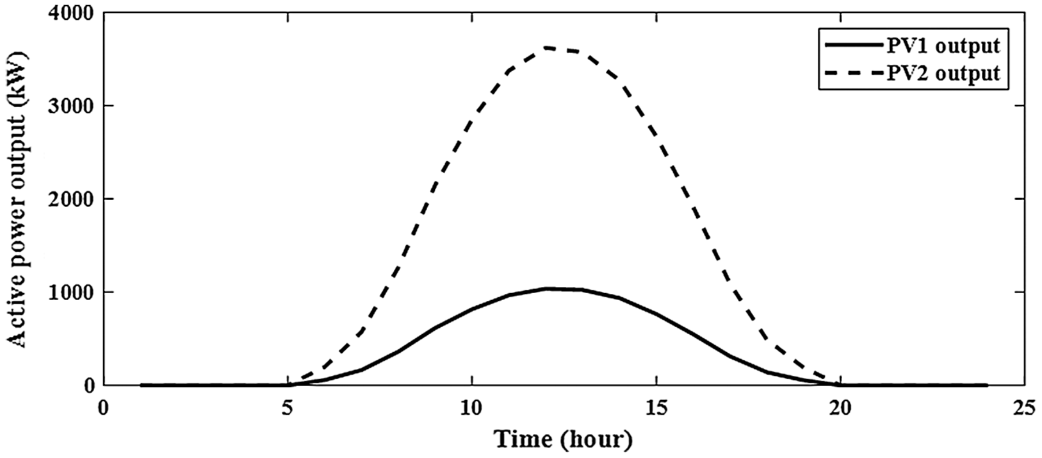
Figure 12: Output of PV for integrating 2-PV with 2-BES in distribution network
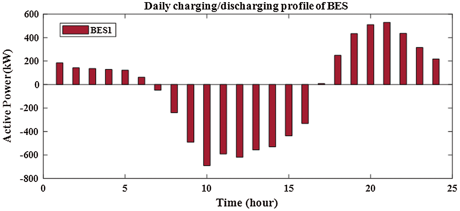
Figure 13: Output of BES1 for integrating 2-PV with 2-BES in distribution network
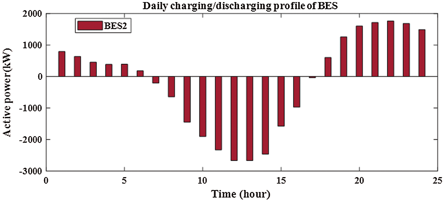
Figure 14: Output of BES2 for integrating 2-PV with 2-BES in distribution network
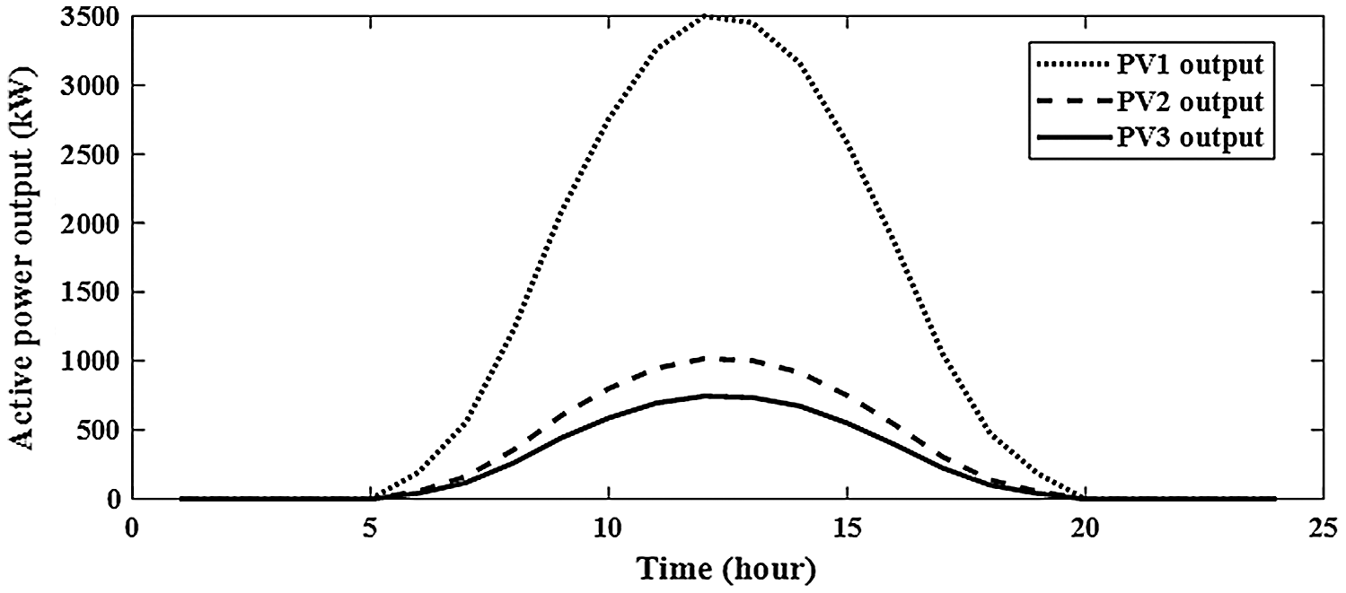
Figure 15: Output of PV for integrating 3-PV with 3-BES in distribution network
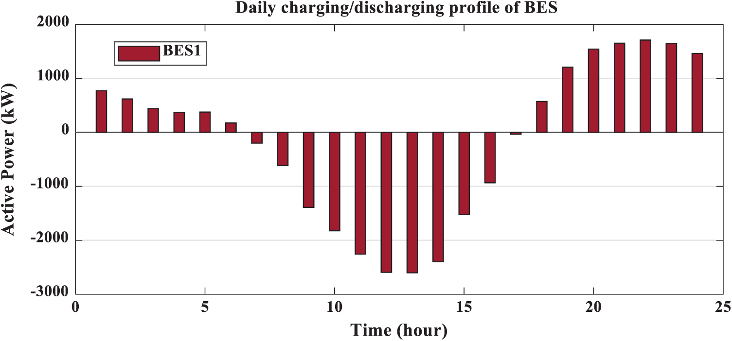
Figure 16: Output of BES1 for integrating 3-PV with 3-BES in distribution network

Figure 17: Output of BES2 for integrating 3-PV with 3-BES in distribution network
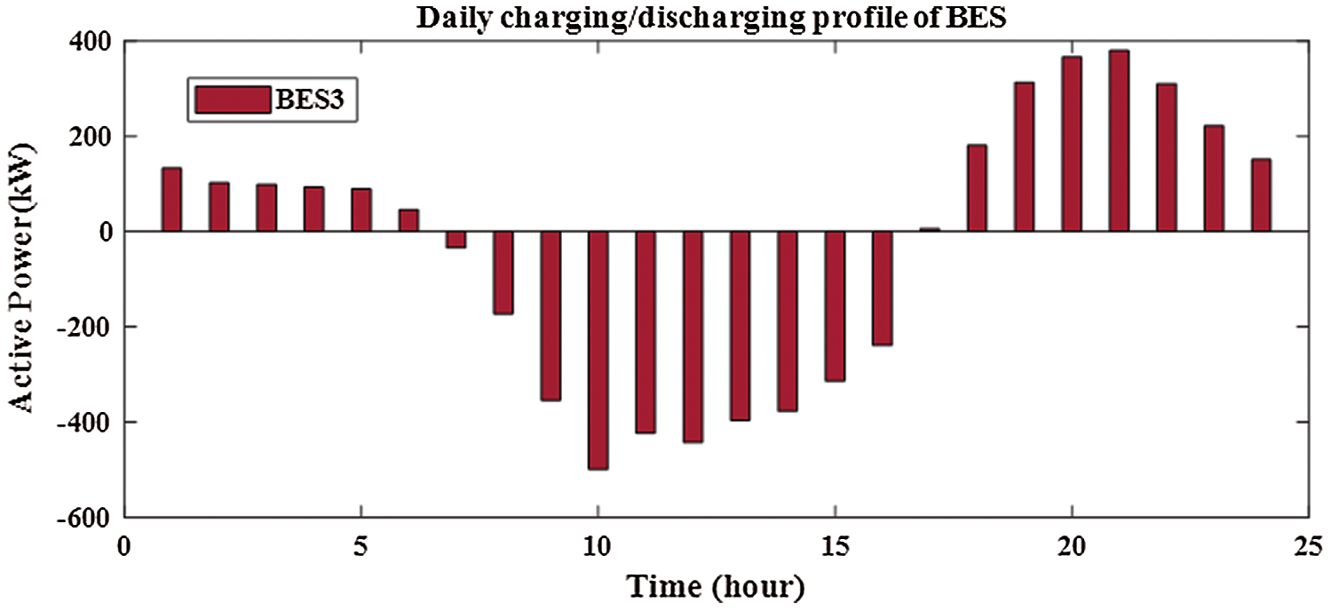
Figure 18: Output of BES3 for integrating 3-PV with 3-BES in distribution network
This paper has proposed a new application of Slime Mould Algorithm to deetermine the optimal allocation of PV alone or with BES considering uncertainty in distribution network. The simulation results proved that SMA has an effective feedback to avoid the local solution and go to the global solution so far. BES is installed with PV to convert PV from non-dispatchable source into dispatchable source. Therefore, BES is used to inject energy to the grid when PV output is low or during the night. The total active power loss during 24-hours is used as single objective function under uncertainty for PV output and system load. The system load is modeled for three types of load that can be defined as residential, industrial and commercial loads. PLSF is used to determine the best buses for installing PV and BES in RDS. From obtained results, the reduction in real power loss by installing one, two and three PV alone in RDS are 18.6%, 20.7% and 21.1%, respectively. Also, the reduction in real power loss by installing one, two and three PVwith BES in RDS are 61.9%, 67.1% and 68.1%, respectively. From simulation results, installing multiple PV alone or with BES achieves superiorsolutions than installing one PV alone or with BES in RDS. Also, integration of PV with BES achieves superior solutions than installing PV alone in distribution network. Integration of PV and BES reduces the system power loss, increases the system capacity and enhances the system voltage.
Funding Statement: This work was supported by “Development of Modular Green Substation and Operation Technology” of the Korea Electric Power Corporation (KEPCO).
Conflicts of Interest: The authors declare that they have no conflicts of interest to report regarding the present study.
1. F. Martins, C. Felgueiras, M. Smitkova and N. Caetano, “Analysis of fossil fuel energy consumption and environmental impacts in european countries,” Energies, vol. 12, no. 6, pp. 964, 2019. [Google Scholar]
2. V. R. VC, “Optimal renewable resources placement in distribution networks by combined power loss index and whale optimization algorithms,” Journal of Electrical Systems and Information Technology, vol. 5, no. 2, pp. 175–191, 2018. [Google Scholar]
3. Z. Abdmouleh, A. Gastli, L. Ben-Brahim, M. Haouari and N. A. Al-Emadi, “Review of optimization techniques applied for the integration of distributed generation from renewable energy sources,” Renewable Energy, vol. 113, pp. 266–280, 2017. [Google Scholar]
4. J. Paska, P. Biczel and M. Kłos, “Hybrid power systems–an effective way of utilising primary energy sources,” Renewable Energy, vol. 34, no. 11, pp. 2414–2421, 2009. [Google Scholar]
5. A. Raheem, “Renewable energy deployment to combat energy crisis in Pakistan,” Energy, Sustainability and Society, vol. 6, no. 1, pp. 1–13, 2016. [Google Scholar]
6. M. Rizwan, G. Mujtaba, S. A. Memon, K. Lee and N. Rashid, “Exploring the potential of microalgae for new biotechnology applications and beyond: A review,” Renewable and Sustainable Energy Reviews, vol. 92, pp. 394–404, 2018. [Google Scholar]
7. M. Yang and X. Huang, “Ultra-short-term prediction of photovoltaic power based on periodic extraction of PV energy and LSH algorithm,” IEEE Access, vol. 6, pp. 51200–51205, 2018. [Google Scholar]
8. A. K. Arani, G. Gharehpetian and M. Abedi, “Review on energy storage systems control methods in microgrids,” International Journal of Electrical Power & Energy Systems, vol. 107, pp. 745–757, 2019. [Google Scholar]
9. S. Li, H. Chen, M. Wang, A. A. Heidari and S. Mirjalili, “Slime mould algorithm: A new method for stochastic optimization,” Future Generation Computer Systems, vol. 111, pp. 300–323, 2020. [Google Scholar]
10. J.-H. Teng, S.-W. Luan, D.-J. Lee and Y.-Q. Huang, “Optimal charging/discharging scheduling of battery storage systems for distribution systems interconnected with sizeable PV generation systems,” IEEE Transactions on Power Systems, vol. 28, pp. 1425–1433, 2012. [Google Scholar]
11. Nottrott, A., J. Kleissl and B. Washom, “Energy dispatch schedule optimization and cost benefit analysis for grid-connected, photovoltaic-battery storage systems,” Renewable Energy, vol. 55, pp. 230–240, 2013. [Google Scholar]
12. L. A. Wong, V. K. Ramachandaramurthy, S. L. Walker, P. Taylor and M. J. Sanjari, “Optimal placement and sizing of battery energy storage system for losses reduction using whale optimization algorithm,” Journal of Energy Storage, vol. 26, pp. 100892, 2019. [Google Scholar]
13. A. Fathy and A. Y. Abdelaziz, “Grey wolf optimizer for optimal sizing and siting of energy storage system in electric distribution network,” Electric Power Components and Systems, vol. 45, pp. 601–614, 2017. [Google Scholar]
14. M. Dixit, P. Kundu and H. R. Jariwala, “Optimal placement of photo-voltaic array and electric vehicles in distribution system under load uncertainty,” in 2017 IEEE Power & Energy Society General Meeting, Chicago, IL, USA, pp. 1–5, 2017. [Google Scholar]
15. U. Eminoglu and M. H. Hocaoglu, “Distribution systems forward/backward sweep-based power flow algorithms: A review and comparison study,” Electric Power Components and Systems, vol. 37, no. 1, pp. 91–110, 2008. [Google Scholar]
16. H. Abdel-Mawgoud, S. Kamel, M. Ebeed and A.-R. Youssef, “Optimal allocation of renewable DG sources in distribution networks considering load growth,” in 2017 Nineteenth Int. Middle East Power Systems Conf., Cairo, Egypt, IEEE, pp. 1236–1241, 2017. [Google Scholar]
17. M. Aman, G. Jasmon, A. Bakar and H. Mokhlis, “A new approach for optimum simultaneous multi-DG distributed generation units placement and sizing based on maximization of system loadability using HPSO (hybrid particle swarm optimization) algorithm,” Energy, vol. 66, pp. 202–215, 2014. [Google Scholar]
18. E. Lopez, H. Opazo, L. Garcia and P. Bastard, “Online reconfiguration considering variability demand: Applications to real networks,” IEEE Transactions on Power Systems, vol. 19, no. 1, pp. 549-553, 2004. [Google Scholar]
19. S. G. Casper, C. O. Nwankpa, R. W. Bradish, H.-D. Chiang, C. Concordia et al., “Bibliography on load models for power flow and dynamic performance simulation,” IEEE Transactions on Power Systems, vol. 10, no. 1, pp. 523-538, 1995. [Google Scholar]
20. H. Abdel-Mawgoud, S. Kamel, M. Khasanov and T. Khurshaid, “A strategy for PV and BESS allocation considering uncertainty based on a modified Henry gas solubility optimizer,” Electric Power Systems Research, vol. 191, pp. 106886, 2021. [Google Scholar]
21. D. Q. Hung, N. Mithulananthan and R. Bansal, “Integration of PV and BES units in commercial distribution systems considering energy loss and voltage stability,” Applied Energy, vol. 113, pp. 1162–1170, 2014. [Google Scholar]
22. K. Muthukumar and S. Jayalalitha, “Optimal placement and sizing of distributed generators and shunt capacitors for power loss minimization in radial distribution networks using hybrid heuristic search optimization technique,” International Journal of Electrical Power & Energy Systems, vol. 78, pp. 299–319, 2016. [Google Scholar]
23. J. Savier and D. Das, “Impact of network reconfiguration on loss allocation of radial distribution systems,” IEEE Transactions on Power Delivery, vol. 22, no. 4, pp. 2473–2480, 2007. [Google Scholar]
24. H. Abdel-Mawgoud, S. Kamel, M. Ebeed and M. M. Aly, “An efficient hybrid approach for optimal allocation of DG in radial distribution networks,” in 2018 Int. Conf. on Innovative Trends in Computer Engineering, Aswan, Egypt, IEEE, pp. 311–316, 2018. [Google Scholar]
25. S. Kansal, V. Kumar and B. Tyagi, “Hybrid approach for optimal placement of multiple DGs of multiple types in distribution networks,” International Journal of Electrical Power & Energy Systems, vol. 75, pp. 226–235, 2016. [Google Scholar]
 | This work is licensed under a Creative Commons Attribution 4.0 International License, which permits unrestricted use, distribution, and reproduction in any medium, provided the original work is properly cited. |