Computers, Materials & Continua DOI:10.32604/cmc.2021.016713
Article

A Mixture Model Parameters Estimation Algorithm for Inter-Contact Times in Internet of Vehicles

Cheng Gong1,2, Xinzhu Yang1, Wei Huangfu3,4,* and Qinghua Lu5

1School of Computer and Communication Engineering, University of Science and Technology Beijing, Beijing, 100083, China
2Beijing Advanced Innovation Center for Materials Genome Engineering, School of Computer and Communication Engineering, University of Science and Technology Beijing, 100083, China
3Shunde Graduate School of University of Science and Technology Beijing, Foshan City, 528300, Guangdong, China
4Beijing Engineering and Technology Center for Convergence Networks and Ubiquitous Services, University of Science and Technology Beijing, Beijing, 100083, China
5Commonwealth Scientific and Industrial Research Organization, Canberra, 2600, Australia
*Corresponding Author: Wei Huangfu. Email: huangfuwei@ustb.edu.cn
Received: 08 January 2021; Accepted: 09 February 2021

Abstract: Communication opportunities among vehicles are important for data transmission over the Internet of Vehicles (IoV). Mixture models are appropriate to describe complex spatial-temporal data. By calculating the expectation of hidden variables in vehicle communication, Expectation Maximization (EM) algorithm solves the maximum likelihood estimation of parameters, and then obtains the mixture model of vehicle communication opportunities. However, the EM algorithm requires multiple iterations and each iteration needs to process all the data. Thus its computational complexity is high. A parameter estimation algorithm with low computational complexity based on Bin Count (BC) and Differential Evolution (DE) (PEBCDE) is proposed. It overcomes the disadvantages of the EM algorithm in solving mixture models for big data. In order to reduce the computational complexity of the mixture models in the IoV, massive data are divided into relatively few time intervals and then counted. According to these few counted values, the parameters of the mixture model are obtained by using DE algorithm. Through modeling and analysis of simulation data and instance data, the PEBCDE algorithm is verified and discussed from two aspects, i.e., accuracy and efficiency. The numerical solution of the probability distribution parameters is obtained, which further provides a more detailed statistical model for the distribution of the opportunity interval of the IoV.

Keywords: Internet of vehicles; opportunistic networks; inter-contact times; mixture model; parameters estimation

1  Introduction

The concept of the Internet of Vehicles (IoV) is closely related to the Internet of Things (IoT) [1–5]. It takes vehicles as the objects of information perception and control. With the help of the new generation of information and communication technologies, the IoV realizes the network connections among the vehicles, people, roads, and service platforms. Thus improve the vehicle driving experience, traffic efficiency, and social traffic service level. The IoV is one of the important branches of the opportunity network [6]. Since vehicles are usually in motion, the instantaneous opportunity communication formed when two vehicles meet is an important way of data transmission in the IoVs. The statistical model of inter-contact times is one of the basic problems of the IoVs [7].

Communication opportunity interval is affected by many factors, including but not limited to vehicle movement model and location distribution, vehicle density, broad geographic distribution, communication accessibility, etc. The previous scholars mainly considered establishing the vehicle movement model and mine the statistical model of communication opportunity interval through theory or simulation. In a Random Waypoint Mobility (RWM) model [8], it was found through simulation that the inter-contact time interval of moving points obeyed exponential distribution [9]. Based on the RWM model and a Random Direction Mobility (RDM) model [10], it was proved that in a finite boundary movement space, the inter-contact time interval was an exponential distribution, while in the unbounded condition, the inter-contact time interval was an approximate power-law distribution [11].

With the development of big data technology, more scholars tended to collect the actual spatial-temporal data sets of vehicle movement, and then used big data mining techniques to determine the statistical model of the data [12,13]. References [14–17] analyzed the inter-contact time interval extracted from the movement trajectory data of buses and taxis in Beijing and Shanghai, respectively. Reference [14] held that the inter-contact time interval of the taxi approximately follows the exponential distribution. References [15,16] both believed that it was a segmented distribution. Only reference [17] proposed that it was the mixture normal distribution. Although the above conclusions based on spatial-temporal big data were not consistent, most of them adopted single statistical distribution or segmented statistical distribution for data analysis. In fact, the IoV are affected by many factors. The sample data of the vehicle movement trajectory is complex and changeable, which may come from a population with different properties. Therefore, a single statistical distribution is difficult to describe the characteristics of actual data. However, the segmented distribution model to describe the vehicle inter-contact time interval is essentially a superficial description of the overall sampled data, so it is difficult to express the complex composition contained in the data.

For the mixture statistical distribution of spatial-temporal big data, a parameter estimation algorithm with low computational complexity based on Bin Count (BC) and Differential Evolution (DE) (PEBCDE) is proposed. BC is used to count all data in a small number of intervals, and a small number of calculated values are used as statistics for the next step of parameter estimation. DE is used to solve nonlinear optimization problems similar to the Expectation Maximization (EM) algorithm [18]. Due to the adoption of BC and DE algorithms, although the accuracy is lower than the EM algorithm, a faster parameter estimation of the statistical model for vehicle inter-contact times is realized. Based on this characteristic, the PEBCDE algorithm proposed in this paper can be used for the online calculation of vehicle-mounted systems. The real-time data received by the vehicles are further calculated to improve the model and obtain more accurate parameter estimation results. In addition, BC parameters can be adjusted to control the accuracy of the algorithm, to optimize the balance between calculated amount and accuracy.

The rest of this paper is arranged as follows. Section 2 describes the related work. Sections 3 and 4 introduce the system model and the algorithm. Analysis and simulation results will be described and displayed in Section 5. Section 6 gives the conclusions of this paper and an outlook for future work.

2  Related Work

For the estimation of a high-dimensional latent variable model, a novel semi-stochastic variance-reduced gradient designed for the Q-function in the EM algorithm was proposed [19]. Compared with the state-of-the-art algorithm, the new algorithm had a certain reduction in the overall computational complexity. Reference [20] modified the EM algorithm, by attaching a truncation step to the expectation step (E-step) and maximization step (M-step), the convergence rate was effectively improved. According to the modified algorithm, the article also gave a decorrelated score statistic about the low dimensional components of the high dimensional parameters.

Reference [21] focused on global convergence rates for stochastic EM methods. In a sufficient statistics space, the EM method can be studied as a scaled-gradient method. On this basis, the author introduced a new incremental version. For a particular model, such as a mixture model of two Gaussians, it had been researched [22]. The article proved the convergence of the sequence of iterates in that model. The author also studied the initial parameter settings. Inspired by variance reduced stochastic gradient descent algorithms, Variance Reduced Stochastic EM (sEM-vr) algorithm was developed [23]. The sEM-vr computed the full batch expectation as a control variate, which reduced the variance of minibatch. Comparing with other gradient-based and Bayesian algorithms, this algorithm achieved a faster convergence speed. Given low-rank mixture regression and regression with missing covariates, it specialized in a general framework [24]. Using the state-of-the-art high-dimensional prescriptions to regular the M-step did not guarantee balance. Aregularization method was proposed considering optimization and statistical error.

The actual spatial-temporal big data often have missing or hidden variables, the traditional methods are difficult to accurately estimate the parameters, and the data may come from different populations. The single distribution model cannot accurately reflect the nature of the data, and it is difficult to mine the effective information of the data. A more reasonable approach is to explore the mixture distribution model of data [25]. The mixture distribution model is a combination of several different statistical distributions according to a certain probability. It is a new combination model combining the properties and characteristics of multiple branches. The mixture distribution model can simulate a large amount of data effectively and make the data distribution model more accurate.

At present, the EM algorithm is usually used for the parameter estimation of mixture statistical distribution modeling [26,27]. It is one of the classical algorithms in the field of data mining and solves the problem that the maximum likelihood estimation is difficult to optimize due to the hidden variables in the actual statistical model. However, the EM algorithm needs to iterate several times to achieve the ideal effect, and each iteration process requires the participation of all data. Therefore, the algorithm has high computational complexity and it is difficult to adapt to the massive spatiotemporal big data scene. Besides, the addition of probability is introduced into the mixture distribution, which calculates logarithmic likelihood very complicated and difficult to obtain closed solutions. As a result, every step of EM iteration becomes a sub-problem of nonlinear optimization, and the computational complexity of EM is increased.

In this paper, BC and DE are introduced to reduce the computational complexity of mixture distribution parameter estimation. Bin counting and DE based on a small amount of data are used to replace the EM algorithm with a large number of data to realize the optimization of the opportunity interval distribution model of the IoVs.

3  System Model

In this paper, based on the longitude and latitude trajectory data of Beijing taxis in May 2010, the algorithm of data cleaning and extraction of inter-contact times interval is presented [16]. Assume that a large sample set X={x1,x2,…,xN} of data has been obtained, where the sample data xi is the time interval in seconds between a communication opportunity and a previous communication opportunity for the same car. Suppose the probability density function f(x) of the mixture statistical model is given by

f(x)=∑i=1kαifi(x),(1)

where, k denotes the number of branches, fi(x) denotes the probability density function of the ith branch, and αi denotes the corresponding weight coefficient with ∑i=1kαi=1, 0≤αi≤1.

The EM algorithm is widely used in parameter estimation of mixture models. The likelihood function can be simplified by introducing suitable potential data. It first assumes that the known observed data of the total sample number N is X, and the potential data is Y={y1,y1,…,yi,…,yn}, where yi={yi1,yi2,…,yik} is a binarization vector. In yi, only one element is 1, and the remaining elements are 0, indicating which branch of the sampled data ti comes from k branches of the mixture distribution. If yi is generated from the pth branch, then yip = 1 and the other elements are 0. In general, Y is unknown. The EM algorithm assumes the existence of complete data set {X,Y} and estimates the unknown parameter θ in the model through continuous iterative optimization of Step E and Step M. The steps are as follows.

(1) Set the initial value θ(0).

(2) Step E: Calculate the conditional expectation of the likelihood function based on the complete data set of the hidden variable Y, denoted as the auxiliary function Q.

Q(θ;θ(m))=EY[lnf(X,Y;θ∣X,θ(m))],(2)

where θ(m) denotes the unknown statistical parameter of the mth iteration.

(3) Step M: Evaluate θ(m+1) to satisfy

Q(θ(m+1);θ(m))= maxQ(θ;θ(m)).(3)

The operations of Step E and Step M above are iterated alternately until ∥θ(m+1)-θ(m)∥ is sufficiently small, and the last θ is the parameter estimate of the mixture distribution model. The main purpose of the EM algorithm is to provide a simple iterative algorithm to calculate the posterior density function. Because the algorithm is simple and stable, it is often used to estimate the parameters of mixture statistical models. However, the EM algorithm is easy to fall into local optimal, which involves all the data in the data set. The time complexity is proportional to the amount of data. When the amount of data is large, the calculation speed is slow.

The basic flow of a parameter estimation algorithm based on BC and DE proposed in this paper is as follows: (1) First, the total sample data is segmented according to a certain interval, and the number of sampled data in each segment is counted. The statistical probability of each segment is calculated by the mixture distribution probability density function (including parameters), and the probability of event occurrence is calculated by multinomial distribution; (2) the event probability calculated in the previous step is taken as the objective function, and the parameter value at the maximum of the objective function is iterated through DE algorithm.

4  Design of the PEBCDE Algorithm

4.1 Segment and Calculate the Maximum Probability Objective Function

Suppose the probability density function of the total data set is f(x), and there are N data points. The data is divided into m segments, also referred to as bins. As shown in Fig. 1, the number of data values in interval [t0,t1] is n1, the number of data values in interval [t1,t2] is n2, and so on, the number of data values in interval [tm-1,tm] is nm. It is assumed that the above interval segmentation can be determined according to prior knowledge or user demands, and the interval can be uniformly divided or non-uniformly divided.

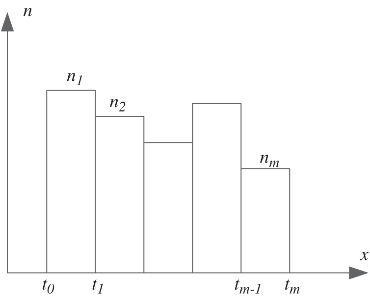
Figure 1: Segmental statistical schematic diagram of the sampled data

If special cases such as the existence of impulse function in probability distribution are not considered, then the probability of data points in the interval [ti-1,ti] is definite integral as

Pi(θ)=∫ti-1tif(x;θ)dx.(4)

The probability that ni out of N data points are in the interval [ti-1,ti] is CNni⋅Pi(θ)ni⋅(1-Pi(θ))N-ni.

According to the multinomial distribution, the occurrence probability P is exactly given as

P(n1,n2,…,nm,θ)={N!n1!⋯nk!P1(θ)n1⋯Pm(θ)nm,∑i=1mni=N0,else.(5)

The time complexity of this step is O(N), and the sampled data needs to be traversed. In the subsequent operation, only the statistic {n1,n2,…,nm} needs to be considered. Here, m is small compared with N, so the scale of data to be processed is greatly reduced. In this step, data within the same interval cannot be distinguished due to interval statistics. Therefore, if the interval is too large, the accuracy of the algorithm will be affected.

4.2 Solve the Estimated Parameters by DE

DE algorithm is a heuristic parallel search method based on group difference. In this step, DE algorithm is used to solve the estimated parameters so that Eq. (5) can obtain the maximum value. First, we initialize the population. In the solution space, M individuals are generated randomly and uniformly, and each individual is composed of K chromosomes. As the 0th generation population, the definition is as follows,

Zi(0)={zi,1(0),zi,2(0),…,zi,K(0)},i=1,2,…,M.(6)

Mutation operation:

In the gth iteration, individuals Zp1(g), Zp2(g) and Zp3(g) are randomly selected from the population for the individual Zi(g)={zi,1(g),zi,2(g),…,zi,K(g)}, and p1≠p2≠p3≠i. Then, the dth dimensional position updating formula is

Hi(g)=Zp1(g)+F⋅(Zp2(g)-Zp3(g)),(7)

where F denotes the scaling factor used to control the influence of the difference factor.

Crossover operation:

Crossover operation increases the diversity of population as follows,

Vi,j(g)={Hi,j(g),rand(0,1)≤crzi,j(g),else,(8)

where cr∈[0,1] denotes the crossover probability.

After completing the mutation and crossover operation, Vi(g) or Xi(g) is selected as Xi(g+1) according to the evaluation function.

Xi(g+1)={Vi(g),iff(Vi(g))<f(Xi(g))Xi(g),else.(9)

The flow of DE algorithm is shown in Fig. 2.

The size of the statistic values that DE algorithm needs to process at each step is m, much smaller than N. Therefore, the algorithm is fast in solving the problem and is very suitable for solving the probability distribution type where it is difficult to find the closed solution. When the number of iterations and individuals are fixed, the time complexity of DE algorithm is only related to the number of segments m, which is close to O(m). This is independent of the overall data size N and greatly reduces the running time. At the same time, parameter estimation for the mixture statistical model of big data can be more accurate.

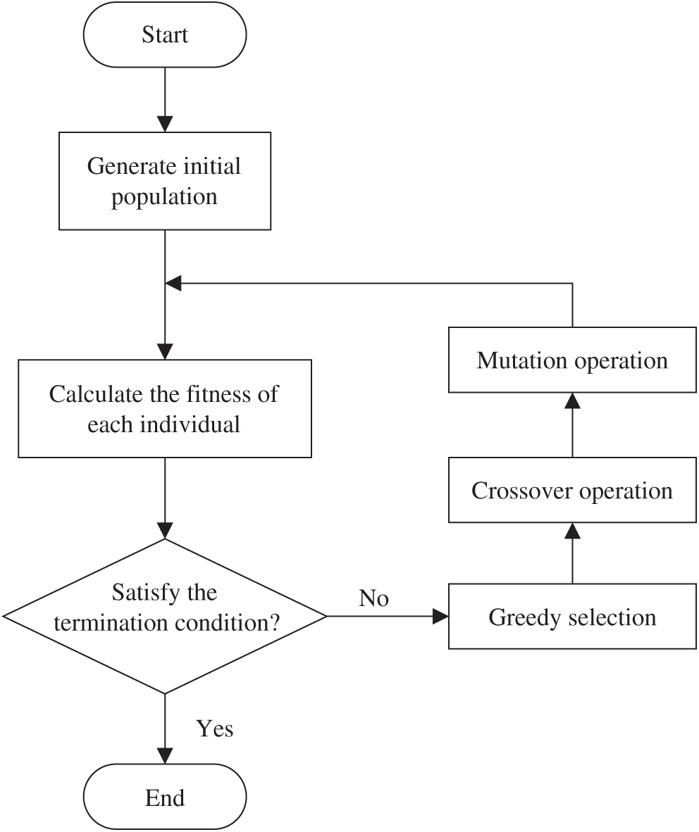
Figure 2: The flow of DE algorithm

5  Performance Analysis

This section analyzes and verifies the effectiveness of the proposed algorithm in the system model. Firstly, the correctness of the algorithm is verified and the accuracy of the algorithm is analyzed. Correctness is verified by comparing the similarity between the given model data and the evaluation model data. The accuracy of the algorithm is observed by modeling and analyzing the ideal data. Based on ensuring the effectiveness and availability of the algorithm, we further apply the algorithm to the actual data set to analyze and verify the actual effect of the PEBCDE algorithm on the movement trajectory data of Beijing taxis. Then, we compare the operation efficiency of the traditional EM algorithm and the proposed PEBCDE algorithm under different parameters, and summarize the performance of the algorithm as a whole.

The simulation experiment is implemented in Python (version 3.7.3) and on an AMD RyzenTM7 3700X processor with 3.60 GHz CPU 16 GB RAM running on the platform Microsoft Window 10.

5.1 Correctness and Accuracy Verification

In this subsection, the simulated data obey a Gaussian mixture distribution with N=1×103, and its probability density function is set as f(x)=α112πσ1 exp(-(x-μ1)22σ12)+(1-α1)12πσ2 exp(-(x-μ2)22σ22). A distribution-based statistical modeling algorithm is used to estimate the parameters of the statistical model. First, let us divide the data into m = 500 bins. In the DE algorithm, the scaling factor is 0.7, and the crossover probability is 0.5. The initial positions are uniformly distributed in the solution space, and the parameters of the mixture Gaussian distribution can be well estimated after about 100 iterations. Simulation parameters are shown in Tab. 1.

The parameters of the statistical model obtained by the PEBCDE algorithm are α1′=0.2717, μ1′=2.0062, σ1′=0.7034, μ2′=3.9583, σ2′=0.6199. Comparing the newly generated data of the model obtained by the PEBCDE algorithm with the data of the original model, the Complementary Cumulative Distribution Function (CCDF) is obtained. The results are shown in Fig. 3. It can be seen that the distribution functions of the two models are similar. In order to better evaluate the effect of the model generated by the algorithm, Goodness of Fit is introduced. The calculation results show that the KS test statistic is 0.017 and the p-value is 0.932, which proves the correctness of the algorithm.

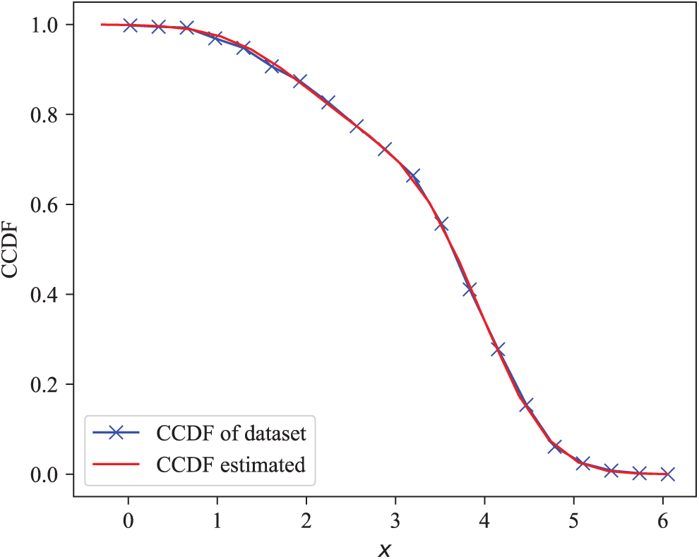
Figure 3: Modeling and comparison of simulation data

The specific iteration of some parameters is shown in Fig. 4. The solid lines represent the actual value of parameters, and the lines with markers represent the value change of the estimated parameter. Each parameter oscillates around the actual value and converges.

Figure 4: The convergence of mean values of both branches per iteration

In the initial stage of data processing, the PEBCDE algorithm needs to segment all the data. The difference in the number of bins leads to different degrees of information loss of part of the raw data, resulting in the different effects on the calculation accuracy. However, the process can also be speeded up, allowing users to adjust the accuracy of calculations to suit their specific needs. Kolmogorov Smirnov (KS) test is used to evaluate the accuracy of the model obtained by the algorithm. The results are shown in Fig. 5. It can be clearly seen that the accuracy of the algorithm has been improved with the increase of the number of bins. It is important to note that the more the number of bins is, the better the algorithm performs. Therefore, after convergence, the KS statistical result with 32 bin is slightly higher than that with 8 bin. This shows that when the number of bins reaches a certain degree, the basically accurate results based on the segmented data can be achieved.

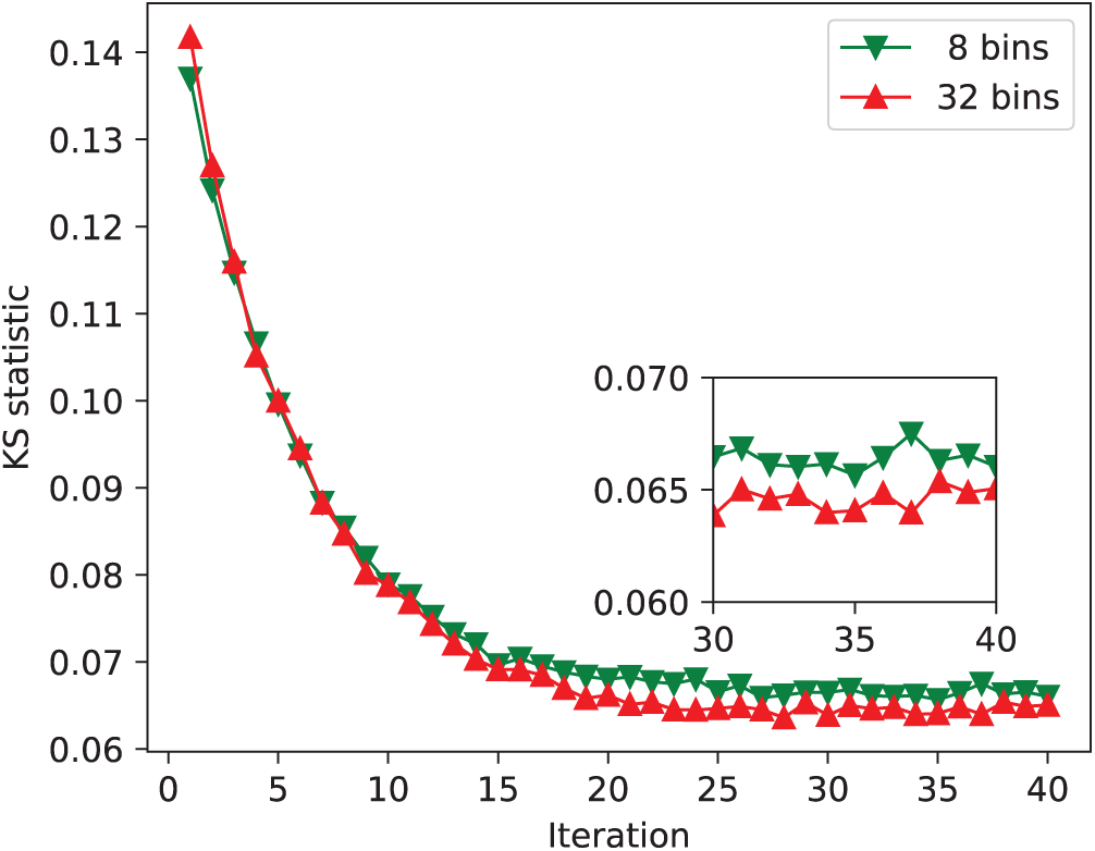
Figure 5: Comparison of KS statistics with different bin counts

5.2 Analysis of Actual Taxi Data

Based on the latitude and longitude trajectory data of Beijing taxis in May 2010, this subsection conducted statistical modeling for the time interval of the IoV communication opportunities. Taking as an example the trajectories of, 100 taxis which were randomly selected from all the data sets, we analyzed the statistical model in the case of the number of vehicles mentioned above.

Through multiple tests and analysis, we believe that the communication opportunity interval between vehicles obeys the mixture of lognormal distribution. The statistical model of different vehicle densities can be fitted with the Gaussian mixture distribution of different parameters. Fig. 6 showed the KS statistics of the actual values under different bin counts and algorithms. All the fitted parameters of the Gaussian mixture distribution passed KS test, and the fitting conditions were good.

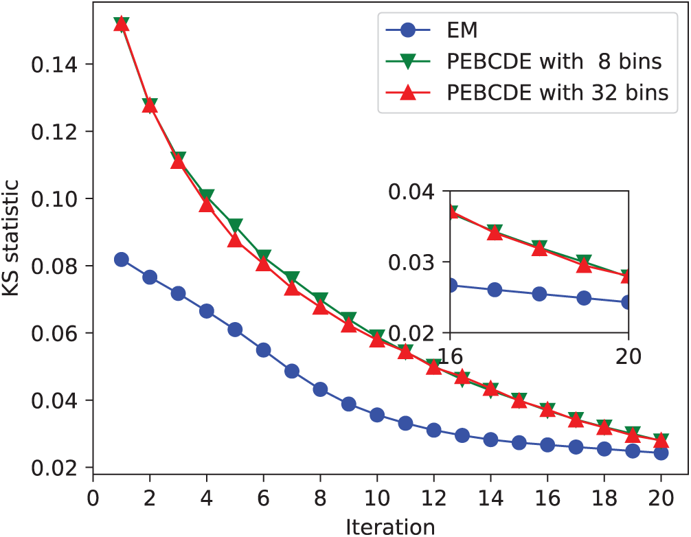
Figure 6: Taxi real communication opportunity interval modeling comparison

If the time span of a single iteration is used as the unit, the EM algorithm had the fastest initial speed. After more than 10 iterations, the EM algorithm basically converged, and a relatively ideal result was obtained. By comparison of the results of the PEBCDE algorithm with 8 and 32 bins, it holds that the greater the number of bins is, the faster the PEBCDE algorithm was converges. Then, similar to the EM algorithm, it fell into the near optimal solution after a number of iterations. Here after about 20 iterations, the near optimal solution was obtained.

5.3 Complexity Analysis

The EM algorithm requires all data in the data set to participate in the calculation. When the amount of data is very large, the calculation speed is slow and it is difficult to deal with massive big data scene. This subsection analyzes the operation efficiency of the EM algorithm and the proposed PEBCDE algorithm.

When the EM algorithm is used for parameter estimation of Gaussian mixture model, the responsiveness of sub-model k to the observed data yj needs to be calculated during step E. The number of calculations is the dimension N of the observed data. Considering that the number of iterations is Ni, the time complexity of the algorithm is O(N*Ni). The PEBCDE algorithm needs to use all the observed data in the initial interval division stage. Then, the size of data used in the next step is the number of intervals, i.e., m. When the number of iterations is Ni, the time complexity of the algorithm is O(N+m*Ni). In the case of the same number of iterations, the complexity of the PEBCDE algorithm is less than that of the EM algorithm due to m≪N.

Firstly, let us set the size of the data volume to 1000 and 100000, respectively, to obtain the running times of the EM algorithm and the PEBCDE algorithm. As shown in Fig. 7, when the amount of data was small, EM algorithm runs fast. However, when the amount of data increased to a certain extent, EM algorithm runs slowly. The running time of the PEBCDE algorithm only increase with the increase of the number of segments because the second step, i.e., DE algorithm, is independent of the data size and only related to the number of segments. Thus PEBCDE is highly efficient for mixture statistical modeling of big data.

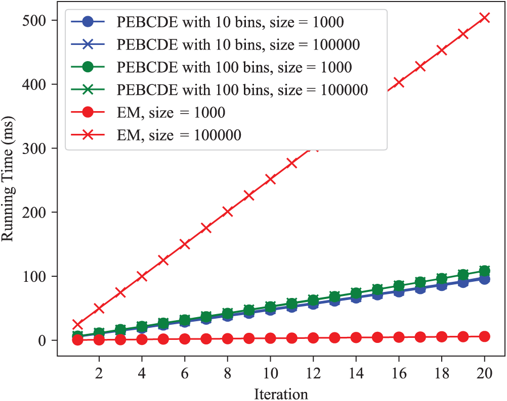
Figure 7: The comparison of running time with different algorithms

6  Conclusion

In this paper, the PEBCDE algorithm based on BC and DE is proposed to overcome the disadvantages of the EM algorithm in parameter estimation of big data mixture model. Through modeling and analysis of simulation data and instance data, the PEBCDE algorithm is verified from two aspects of accuracy and efficiency. The research shows that the computational complexity of the PEBCDE algorithm is significantly reduced. As the increase of data volume, every iteration round of the EM algorithm needs all the data, while the PEBCDE algorithm only needs to traverse all the data once. Therefore, when the amount of data is large, the running time of the PEBCDE algorithm is far less than that of the EM algorithm.

It is worth noting that the PEBCDE algorithm sacrifices precision to some extent compared with the EM algorithm. This is because differences between data within the same interval are ignored after interval calculation. Therefore, the first few moments of the data can be obtained by improving the PEBCDE algorithm combining moment estimation in the first step, and then applied to DE algorithm in the second stage, to further improve the accuracy of this algorithm.

Acknowledgement: We gratefully acknowledge anonymous reviewers who read drafts and made many helpful suggestions.

Funding Statement: This work was supported by the Fundamental Research Funds for the Central Universities (Grant No. FRF-BD-20-11A), and the Scientific and Technological Innovation Foundation of Shunde Graduate School, USTB (Grant No. BK19AF005).

Conflicts of Interest: The authors declare that they have no conflicts of interest to report regarding the present study.

References

 1.  W. Zhang and X. Xi, “The innovation and development of internet of vehicles,” China Communication, vol. 13, no. 5, pp. 122–127, 2016. [Google Scholar]

 2.  B. Mohammed and D. Naouel, “An efficient greedy traffic aware routing scheme for internet of vehicles,” Computers, Materials & Continua, vol. 60, no. 3, pp. 959–972, 2019. [Google Scholar]

 3.  C. Gong, F. Lin, X. Gong and Y. Lu, “Intelligent cooperative edge computing in internet of things,” IEEE Internet of Things Journal, vol. 7, no. 10, pp. 9372–9382, 2020. [Google Scholar]

 4.  H. Hui, C. Zhou, S. Xu and F. Lin, “A novel secure data transmission scheme in industrial internet of things,” China Communication, vol. 17, no. 1, pp. 73–88, 2020. [Google Scholar]

 5.  L. Zhang, W. Cao, X. Zhang and H. Xu, “MAC2: Enabling multicasting and congestion control with multichannel transmission for intelligent vehicle terminal in internet of vehicles,” International Journal of Distributed Sensor Networks, vol. 14, no. 8, pp. 1–20, 2018. [Google Scholar]

 6.  P. Guan and J. Wu, “Effective data communication based on social community in social opportunistic networks,” IEEE ACCESS, vol. 7, pp. 12405–12414, 2019. [Google Scholar]

 7.  E. Hernández-Orallo, J. C. Cano, C. T. Calafate and P. Manzoni, “New approaches for characterizing inter-contact times in opportunistic networks,” Ad Hoc Networks, vol. 52, no. 10, pp. 160–172, 2016. [Google Scholar]

 8.  A. Pramanik, B. Choudhury, T. S. Choudhury, W. Arif and J. Mehedi, “Simulative study of random waypoint mobility model for mobile ad hoc networks,” in 2015 Global Conf. on Communication Technologies, Thuckalay, India, pp. 112–116, 2015. [Google Scholar]

 9.  G. Sharma and R. R. Mazumdar, “Scaling laws for capacity and delay in wireless ad hoc networks with random mobility,” in 2004 IEEE Int. Conf. on Communications (IEEE Cat. No. 04CH37577Paris, France, pp. 3869–3873, 2004. [Google Scholar]

10. G. Carofiglio, C.-F. Chiasserini, M. Garetto and E. Leonardi, “Route stability in MANETs under the random direction mobility model,” IEEE Transactions on Mobile Computing, vol. 8, no. 9, pp. 1167–1179, 2009. [Google Scholar]

11. H. Cai and D. Y. Eun, “Crossing over the bounded domain: from exponential to power-law inter-meeting time in mobile ad hoc networks,” IEEE/ACM Transactions on Networking, vol. 17, no. 5, pp. 1578–1591, 2009. [Google Scholar]

12. G. Nguyen, S. Dlugolinsky, M. Bobák, V. Tran, A. L. García et al., “Machine learning and deep learning frameworks and libraries for large-scale data mining: a survey,” Artificial Intelligence Review, vol. 52, no. 1, pp. 77–124, 2019. [Google Scholar]

13. H. Zhou, G. Sun, S. Fu, X. Fan, W. Jiang et al., “A distributed approach of big data mining for financial fraud detection in a supply chain,” Computers, Materials & Continua, vol. 64, no. 2, pp. 1091–1105, 2020. [Google Scholar]

14. H. Zhu, M. Li, L. Fu, G. Xue, Y. Zhu et al., “Impact of traffic influxes: Revealing exponential intercontact time in urban vanets,” IEEE Transactions on Parallel and Distributed Systems, vol. 22, no. 8, pp. 1258–1266, 2010. [Google Scholar]

15. Y. Li, D. Jin, P. Hui, L. Su and L. Zeng, “Revealing contact interval patterns in large scale urban vehicular ad hoc networks,” ACM SIGCOMM Computer Communication Review, vol. 42, no. 4, pp. 299–300, 2012. [Google Scholar]

16. W. Huangfu, X. Yang, H. Wang and X. Hu, “Modeling the statistical distribution of the inter-contact times for communication opportunities in vehicle networks,” Journal of Beijing University of Posts & Telecommunications, vol. 42, no. 3, pp. 37–43, 2019. [Google Scholar]

17. X. Zhang, J. Kurose, B. N. Levine, D. Towsley and H. Zhang, “Study of a bus-based disruption-tolerant network: Mobility modeling and impact on routing,” in Proceedings of the 13th Annual ACM Int. Conf. on Mobile Computing and Networking, Montréal Québec Canada, pp. 195–206, 2007. [Google Scholar]

18. T. Chen and M. Yeh, “Optimized pid controller using adaptive differential evolution with meanof-pbest mutation strategy,” Intelligent Automation & Soft Computing, vol. 26, no. 3, pp. 407–420, 2020. [Google Scholar]

19. R. Zhu, L. Wang, C. Zhai and Q. Gu, “High-dimensional variance-reduced stochastic gradient expectation-maximization algorithm,” in Proc. of the 34th Int. Conf. on Machine Learning, Sydney, NSW, Australia, pp. 4180–4188, 2017. [Google Scholar]

20. Z. Wang, Q. Gu, Y. Ning and H. Liu, “High dimensional EM algorithm: Statistical optimization and asymptotic normality,” in Advances in Neural Information Processing Systems 28: Annual Conf. on Neural Information Processing Systems 2015, Montreal, Quebec, Canada, pp. 2521–2529, 2015. [Google Scholar]

21. B. Karimi, H.-T. Wai, E. Moulines and M. Lavielle, “On the global convergence of (fast) incremental expectation maximization methods,” in Advances in Neural Information Processing Systems 32: Annual Conf. on Neural Information Processing Systems 2019, Vancouver, BC, Canada, pp. 2833–2843, 2019. [Google Scholar]

22. J. Xu, D. J. Hsu and A. Maleki, “Global analysis of expectation maximization for mixtures of two gaussians,” in Advances in Neural Information Processing Systems 29: Annual Conf. on Neural Information Processing Systems 2016, Barcelona, Spain, pp. 2676–2684, 2016. [Google Scholar]

23. J. Chen, J. Zhu, Y. W. Teh and T. Zhang, “Stochastic expectation maximization with variance reduction,” in Advances in Neural Information Processing Systems 31: Annual Conf. on Neural Information Processing Systems 2018, Montréal, Canada, pp. 7978–7988, 2018. [Google Scholar]

24. X. Yi and C. Caramanis, “Regularized EM algorithms: A unified framework and statistical guarantees,” in Advances in Neural Information Processing Systems 28: Annual Conf. on Neural Information Processing Systems 2015, Montreal, Quebec, Canada, pp. 1567–1575, 2015. [Google Scholar]

25. A. J. A. Nelder and R. W. M. Wedderburn, “Generalized linear models,” Journal of the Royal Statistical Society Series A (General), vol. 135, no. 3, pp. 370–384, 1972. [Google Scholar]

26. G. J. McLachlan and T. Krishnan, The EM Algorithm and Extensions. vol. 382. Hoboken, New Jersey, United States: John Wiley & Sons, 2007. [Google Scholar]

27. F. Mallouli, “Robust em algorithm for iris segmentation based on mixture of gaussian distribution,” Intelligent Automation & Soft Computing, vol. 25, no. 2, pp. 243–248, 2019. [Google Scholar]

This work is licensed under a Creative Commons Attribution 4.0 International License, which permits unrestricted use, distribution, and reproduction in any medium, provided the original work is properly cited.