Computers, Materials & Continua DOI:10.32604/cmc.2021.015524
Article

Classification of Epileptic Electroencephalograms Using Time-Frequency and Back Propagation Methods

Sengul Bayrak1,2,*, Eylem Yucel2, Hidayet Takci3 and Ruya Samli2

1Department of Computer Engineering, Halic University, Istanbul, 34445, Turkey
2Department of Computer Engineering, İstanbul University—Cerrahpasa, Istanbul, 34320, Turkey
3Department of Computer Engineering, Sivas Cumhuriyet University, Sivas, 58140, Turkey
*Corresponding Author: Sengul Bayrak. Email: bayraksengul@ieee.org
Received: 25 November 2020; Accepted: 20 January 2021

Abstract: Today, electroencephalography is used to measure brain activity by creating signals that are viewed on a monitor. These signals are frequently used to obtain information about brain neurons and may detect disorders that affect the brain, such as epilepsy. Electroencephalogram (EEG) signals are however prone to artefacts. These artefacts must be removed to obtain accurate and meaningful signals. Currently, computer-aided systems have been used for this purpose. These systems provide high computing power, problem-specific development, and other advantages. In this study, a new clinical decision support system was developed for individuals to detect epileptic seizures using EEG signals. Comprehensive classification results were obtained for the extracted filtered features from the time-frequency domain. The classification accuracies of the time-frequency features obtained from discrete continuous transform (DCT), fractional Fourier transform (FrFT), and Hilbert transform (HT) are compared. Artificial neural networks (ANN) were applied, and back propagation (BP) was used as a learning method. Many studies in the literature describe a single BP algorithm. In contrast, we looked at several BP algorithms including gradient descent with momentum (GDM), scaled conjugate gradient (SCG), and gradient descent with adaptive learning rate (GDA). The most successful algorithm was tested using simulations made on three separate datasets (DCT_EEG, FrFT_EEG, and HT_EEG) that make up the input data. The HT algorithm was the most successful EEG feature extractor in terms of classification accuracy rates in each EEG dataset and had the highest referred accuracy rates of the algorithms. As a result, HT_EEG gives the highest accuracy for all algorithms, and the highest accuracy of 87.38% was produced by the SCG algorithm.

Keywords: Extracranial and intracranial electroencephalogram; signal classification; back propagation; finite impulse response filter; discrete cosine transform; fractional Fourier transform; Hilbert transform

1  Introduction

Epilepsy is one of the most common neurological disorders in the world [1]. This disorder occurs as epileptic seizures because of the sudden change in electrical activity in the brain [2]. Epileptic seizures were systematically classified by the International League Against Epilepsy (ILAE) [3]. However, there are many unknown parameters for seizures, and it is hard to diagnose the disorder. The information about epilepsy in electroencephalogram (EEG) signals can be used for the diagnosis and treatment of epilepsy [4,5]. However, there are some challenges to using EEG signals. Analysis of the EEG signals is typically performed manually, and there may be subjective consequences [4]. EEG signals are affected by artifact noise that results from activities such as chewing, sweating, blinking, coughing, and other actions. Computer-aided models are used to evaluate, analyze, and classify epileptic EEG signals with high accuracy rates to help reduce these artifacts [6].

The use of databases is an important approach to the analysis of EEGs. In the literature, different computer-aided models using different EEG signal databases have been proposed. A summary of the studies using the BONN EEG database in the literature is presented in Tab. 1.

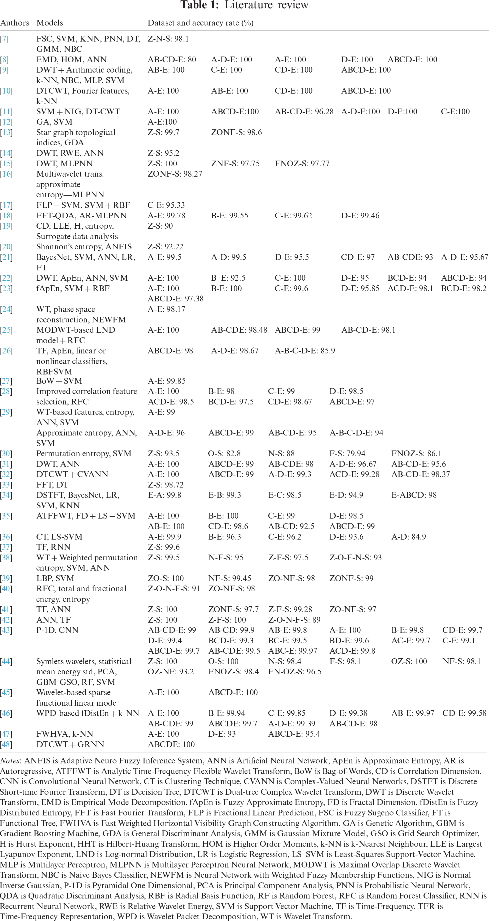
The most commonly used models in the BONN database studies are artificial neural networks (ANN), support vector machine (SVM), k-nearest neighbors (k-NN), and recursive flow classification (RFC) (Tab. 1). They obtained 100% accuracy rates with various datasets such as A-D-E, A-E, ABCD-E, D-E [8], AB-E, C-E, CD-E, ABCD-E [9], A-E, AB-E, CD-E, ABCD-E [10], ABCD-E, A-E, A-D-E, D-E, C-E [11], A-E [12], Z-S [15], A-E, C-E [22], A-E, B-E [23], and A-E [25]. ANN is an information processing system inspired by biological nervous systems that can perform computations at a very high speed if implemented on dedicated hardware. It can adapt itself to learn the knowledge of input signals [15,16,22,38,42]. The SVM classifier is the selected hyperplane that maximizes margins, namely the distance to the nearest training set. Maximizing the margins increases the generalization capabilities of the SVM algorithm in classification, but SVM has relatively low execution speed [29,37,38,43]. k-NN is a simple model that appoints a feature vector to a class according to its nearest neighbor or neighbors [9,10]. The RFC algorithm works by generating multiple decision trees at the training time and subtracting the average estimate of individual trees [25,28].

There are some studies in which these methods achieve 100% success. However, the reported studies do not have the same datasets. The accuracy rate obtained for the method recommended for the problem of classifying Z, O and N, F, S signals, which is needed by clinical experts in our study, is 87.38%. It is the method with the second-best classification accuracy in the literature for this data set. The best result is 99.5% obtained by Ullah et al. [43]. This was obtained from the P-1D analysis combination with a convolutional neural network (CNN). Although the classification accuracies are close in value for these two experiments, the time-frequency features applied in the proposed method are much simpler and have lower computation costs compared to those in other studies. This makes the system developed in the current work more suitable for real-time seizure detection in clinical epilepsy diagnostics.

In this study, three ANN back propagation (ANN-BP) algorithms were used to classify EEG signals to determine the best feature extractor and algorithm. The steps in our study can be summarized as follows. (i) Finite impulse response (FIR) filtering was used for the preprocessing to remove noise from the EEG signals;

(ii) The time-frequency domain features were extracted by discrete continuous transform (DCT), fractional Fourier transform (FrFT), and Hilbert transform (HT);

(iii) The features were obtained from the DCT_EEG, FrFT_EEG, and HT_EEG datasets;

(iv) DCT_EEG, FrFT_EEG, and HT_EEG were classified with the gradient descent with momentum (GDM), scaled conjugate gradient (SCG), and gradient descent with adaptive learning rate (GDA) training algorithms for the extracranial and the intracranial EEG signals; and

(v) Classification accuracy rates were compared for the training algorithms according to the best time-frequency features.

The rest of the paper is organized as follows. The methods of the proposed models are described step by step in Section 2. The experimental results are given in Section 3, and the conclusions of the study are presented in Section 4.

2  Materials and Methods

In this study, the extracranial and intracranial EEG signals were used for classifying the features of the significant time-frequency EEG signals from the ANN-BP algorithms.

2.1 Dataset

The analyzed EEG signals were obtained from the publicly available BONN database [49]. The sampling rate of the EEG signals was 173.61 Hz, and the spectral band of the dilution system is in the range 0.5–85 Hz. The input dataset consisted of five sets {Z, O, N, F, S}, each containing 100 single-channel EEG segments of 23.6 s duration; each data segment contained 4097 samples. In this study, EEG signals, apart from the different recording electrodes, were used for diagnosis epilepsy where the sets of {Z, O} and {N, F, S} were recorded extracranially and intracranially, respectively. The signal classification modeling steps were preprocessing, feature extraction, and classification. {Z, O} sets were taken from surface EEG signal records of five healthy volunteers with open and closed eyes. Signals were measured in two groups at seizure intervals from the hippocampal formation of five patients in the epileptogenic region {F} and the opposite half-sphere of the brain {N}. {S} contained selected seizure activity from all recording areas displaying ictal activity.

2.2 Preprocessing

Preprocessing is a crucial step for the removal of artifacts from EEG signals before extracting significant signal features. Therefore, in this study the FIR filtering method was used to remove artifacts.

FIR filtering has a non-recursive impulse response that has a finite duration of h[n]. The transfer function H[z] of FIR filtering, which contains only zeros and no poles, is always stable. The impulse response is usually an interruption of the infinite impulse response h∞[n] or a finite time section with a window [50]. In the FIR filter, input x[n] and output y[n] are defined by Eqs. (1) and (2).

H(z)=Y(z)/X(z)=∑n=0N-1h[n]z-n (1)

y[n]=∑k=0N-1h[k]x[n-k] (2)

In this study, the structure of the FIR filter for preprocessing shows that the impulse response of Eq. (3) is 4097 points.

h∞[n]=(0.5)nu[n](3)

So, h[n]=h∞(n)R4097[n] was obtained as Eqs. (4) and (5).

R4097[n]=u(n)-u[n-4097] (4)

h[n]=(0.5)nR4097[n] (5)

The FIR filtering structure is shown in Fig. 1.

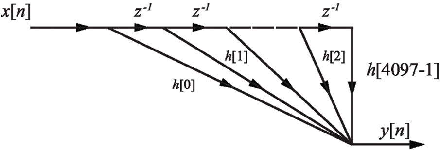
Figure 1: The FIR filtering structure for set of EEG signals

The Kaiser window is crucial for reducing spectral leakage in the analysis of EEG signals that concentrate most of the energy in the amplitude. It is almost optimal, and it depends on the parameter β, which controls its form as described by Eq. (6).

w[n]=I0(1-(2n/N)-1)2I0(β),0≤n≤N(6)

I0 shows the zero order Bessel function, which is measured using the power series expansion as in Eq. (7) described earlier [50].

I0(x)=1+∑k=1∞{(x/2)kk!}2(7)

2.3 Feature Extraction

In this study, significant features for extracranial and intracranial EEG signals were extracted by the time-frequency domain using DCT, FrFT, and HT. These extractions helped to describe significant features of EEG signal components that tend to be complex and chaotic structures. Three datasets were extracted by the time-frequency methods, and three different ANN-BP training algorithms were applied to compare classification accuracy rates.

2.3.1 DCT

DCT is given as an even function f(t) ( t = 0 axis). The results of even functions are the real spectrum. (2N-2) samples are given as x[0],x[1],…,x[2N-3] through even symmetry about n = N −1 as shown in Fig. 2 [51].

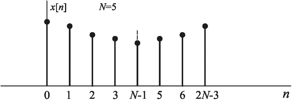
Figure 2: Symmetry EEG signals

x[1]=x[2N-3],x[2]=x[2N-4],…,x[N-2]=x[N]; x[0] and x[N-1] are unique as shown in Eq. (8).

x[k]=x[0]+(-1)kx[N-1]+2∑n=1N-2x[n]cosπN-1nk(8)

2.3.2 FrFT

The purpose of FrFT is transferring signals from the time domain to the frequency domain and to determine the most significant features for the EEG signals. The FrFT of EEG signals, f(t), is given by Eq. (9):

Fa(jω)=∫-∞∞Aajπ[cotαω2/(4π2)-2cscα(ω/2π)t+cotαt2]f(t)dt(9)

where Aa=1-j cot α changes with ω=2πf; ω describes the variable in the transform domain as described in Eq. (10).

Fa(f)=Aajπcotαf2∫−∞∞e−j2π2cscαft+jπωtαt2]f(t)dt(10)

The variable parameter α changes α times π/2, which rotates angle changes from 0 to 2π. In this study, the value of α changed in the interval as 0.1 and 1 the fractional transform is the usual Fourier transform as Eq. (11) as in [52].

Fa(f)=1+j tan αe-jπtan αf2(11)

2.3.3 HT

h(t) is a real impulse response, which is shown in Eq. (12).

H(jω)=HR(jω)+jHI(jω)(12)

H(jω) has been concluded from either HR(jω) or HI(jω). H(jω) is a rational function. Therefore, H(s)=N(s)D(s). H(s) is analytic, and there is no pole in the right half plane.

In this study, it was extracted from filtered EEG signals time-domain HT relations where there were no poles on the jω axis followed by the case of poles on the axis.

D(s) is called a ‘Hurwitz’ polynomial, and it has no zeros for Re(s)>0 [53]. The filtered EEG signals were decomposed 4097 points. The sequence in Fig. 3 represents the EEG signals of a patient as described in Eq. (13).

he[n]=(1/2)[h[n]+h[-n]](13)

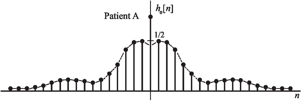
Figure 3: An example EEG signals sequence

2.4 Classification of ANN-BP Training Algorithms

ANN-BP training algorithms are the most widely used algorithms for weight-updating strategies in classification processes [54,55]. The following components were implemented for the training phase of this study: the fully connected Multi-Layer Perceptron (MLP) models for classifying the extracranial {Z, O} and the intracranial {N, F, S} signals.

The EEG datasets obtained from time-frequency methods (DCT, FrFT, and HT) were classified by ANN-BP algorithms.

Initially, the weights (ω) and the biases (b) were set, and the three EEG signal datasets X(4097×500) were given as input. The outputs were the extracranial and intracranial EEG signals with {Z, O, N, F, S} according to momentum (μ). Finally, the output signals were calculated using Eq. (14):

yJ=ϕ(∑i=14097ωjixi+bj)(14)

Three basic training algorithms (GDM, SCG, GDA) were used to show the best classification performances with the effective time-frequency feature descriptor method.

2.4.1 GDM Algorithm

The GDM algorithm allows the neural network model to respond to both local degradation and recent trends on the error surface. The momentum performs as a low-pass filter, which allows the minor features to be ignored on the error surface of the neural network. The learning rate (lr) is the simple gradient descent parameter, and the (μ) parameter describes the amount of momentum. ANN-BP is used to calculate performance (perf) derivatives based on X ’s performance, which is dependent on (ω) and (b) parameters in Eq. (15), and each parameter is set with respect to GDM [56]:

dX=μ×dXprev+lr×(1-μ)×dperf/dX(15)

where dXprev is the previous change according to the (ω) or (b) parameters. The GDM algorithm helps reach the local minimum value faster in the neural network. Momentum is where a temporal element was added to the equation to update the parameters of a neural network. (dX) is the objection function that is being optimized. Essentially, (dX) is the saved gradient calculations or updates to be used in all subsequent updates of a parameter, which is (ω), (b), or activation.

2.4.2 SCG Algorithm

The SCG can train any network as long as its weight and net input. SCG is an effective and fully automated optimization approach for the supervised learning algorithm that represents performance benchmarked against that of the standard ANN-BP. It does not add any user-dependent parameters that are crucial for its success. The algorithm avoids time consuming line search as per the learning iteration and uses a step-size scaling mechanism. The training step size equals the minimum quadratic polynomial fitted to E′(ω^k)Tp^k,E′(ω^k),E′((ω^k)+αk+p^k) [57]. The SCG algorithm is indicated below:

—   Choose the weight vector (ω^1) and scalars 0<σ≤104,0<λ1≤10-6,λ¯1=0.

—   Set p^1=-E′(ω^1),k=1 and success = true.

—   If the success is equal to true, then calculate the second order information as δk=p^kTŝk.

—   If δk≤0, then make the Hessian matrix positive definite as λk=λ¯k.

—   Calculate the step size as αk=μk/δk.

—   Calculate the comparison parameter. Δk=2δk[E(ω^k)-E(ω^k+αkp^k)]/μk2.

—   If Δk≥0, then the successful reduction in error is calculated [82].

—   If the Δk<0.25, then the scale parameter is increased.

—   If the steepest descent direction is not equal to 0, then set k = k + 1 .

2.4.3 GDA Algorithm

The output and error rate of the GDA algorithm are calculated in the neural network model. In each epoch, the new (ω) and (b) parameters are calculated by using the current learning rate. Next, new outputs and errors are calculated. The GDA neural network model, weight, input, and transfer functions are trained by the derivative functions. Each parameter is set according to gradient descent as in Eq. (16).

dX=lr×dperf/dX(16)

In each epoch, the learning rate increases by the lr factor if the performance decreases towards the target [58]. In Eq. (16), ANN-BP is used to calculate performance (perf) derivatives based on X ’s performance, which is dependent on (ω) and (b) parameters. GDA provides a simple approach to change the learning rate over time. It is important to accommodate the differences in the datasets, as it may receive small or large updates depending on how the learning rate is defined. As the learning rate decreases, GDA takes smaller and smaller steps to get faster, because the local minimum value is not exceeded by the large steps.

2.5 Statistical Parameters

Our proposed models were evaluated by computing the statistical parameters of Cohen’s Kappa coefficient and receiver operating characteristic (ROC).

The Kappa Test is a statistical method that measures the reliability of compliance between two or more observers. If the test is between two observers, it is called cohenKappa. Since the variable in which compliance is evaluated is categorical, the applied statistic is non-parametric. Two different probabilities Pr(a) and Pr(e) are calculated when working out the cohenKappa. Pr(a) is the ratio of the observed accuracy to the sum of the two classifiers, and Pr(e) is the probability of this agreement occurring with the expected accuracy. The formula to find cohenKappa is shown in Eq. (17) [59]:

cohenKappa=Pr(a)- Pr(e)1- Pr(e)(17)

An earlier study [59] presented the following comments about the results of the two observers to analyze the obtained cohenKappa values that can be between −1 and +1:

<0: harmony depends only on chance;

0.01–0.20: insignificant compliance;

0.21–0.40: poor compliance;

0.41–0.60: moderate compliance;

0.61–0.80: good fit;

0.81–1.00: very good level of the fit.

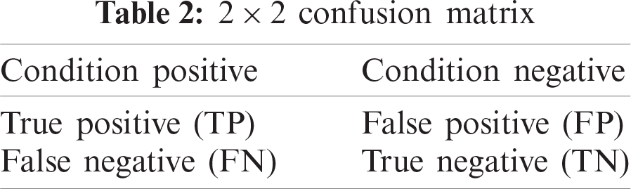
An ROC curve is a graphical plot that shows the classification ability for binary classification. The ROC curve is constructed by plotting the false positive rate (FPR) versus the true positive rate (TPR) for the various threshold settings. Tab. 2 describes TPR and FPR whose formulation is given in Eq. 18 [60].

TPR=∑ TP∑ ConditionPositive;FPR=∑ FP∑ ConditionNegative(18)

The ROC curve can be generated by plotting the cumulative distribution function of the detection probability in the y-axis versus the cumulative distribution function of the false-alert probability on the x-axis. ROC analysis includes tools to perceive models that may be optimal and to reject sub-optimal models independently from the cost case or the class distribution.

3  Experimental Results

In this study, the experiments were performed by using three different EEG signals datasets obtained using the DCT, FrFT, and HT for extracting the significant time-frequency EEG signal features. The experimental research consisted of the following steps:

Step 1: Removing artifacts and noises from signals using the FIR filter;

Step 2: Extracting significant filtered signal features from the time-frequency methods by the DCT, FrFT, and HT;

Step 3: Classifying the extracranial and intracranial signals from the ANN-BP algorithms using the GDM, SCG, and GDA models;

Step 4: Comparing the classification accuracy rates of the models. The structure of the proposed model is shown in Fig. 4. In this study, the Kaiser window was appropriate for reducing the artifacts and noise when convolved by the ideal filter response, leading to a wider transition region selected as 3. The filtered EEG signals, which were the input data, were the values of (4097×500)(n,…,N(1,…,4097)).

The flowchart for obtaining the DCT_EEG dataset is shown in Fig. 5a, and the DCT type was initialized as 1. DCT was obtained as a (4097×500) matrix and can reconstruct a sequence from only a few DCT coefficients accurately. In this study, DCT is important for general data reduction. The flowchart for obtaining the FrFT_EEG dataset is shown in Fig. 5b. Fα(jω) rotated the signals, f(t), and projected into the line of angle, α, in the time-frequency domain. In this study, the value of α could be changed in the interval 0.1–1, and the fractional transform was the usual Fourier transform. This process contributed to the FrFT-based decomposition algorithm when applied to signals. The flowchart for obtaining the HT_EEG dataset is shown in Fig. 5c. The changes of the FFT coefficients corresponded to negative frequencies with zeros, and they were calculated as the inverse FFT value of the result.

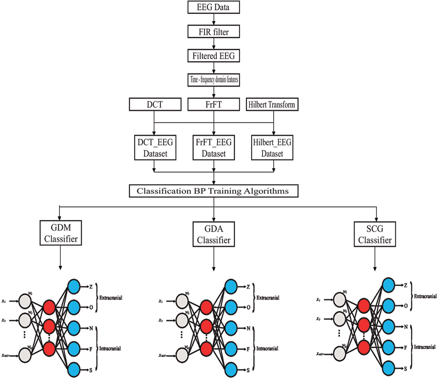
Figure 4: The structure of the proposed model

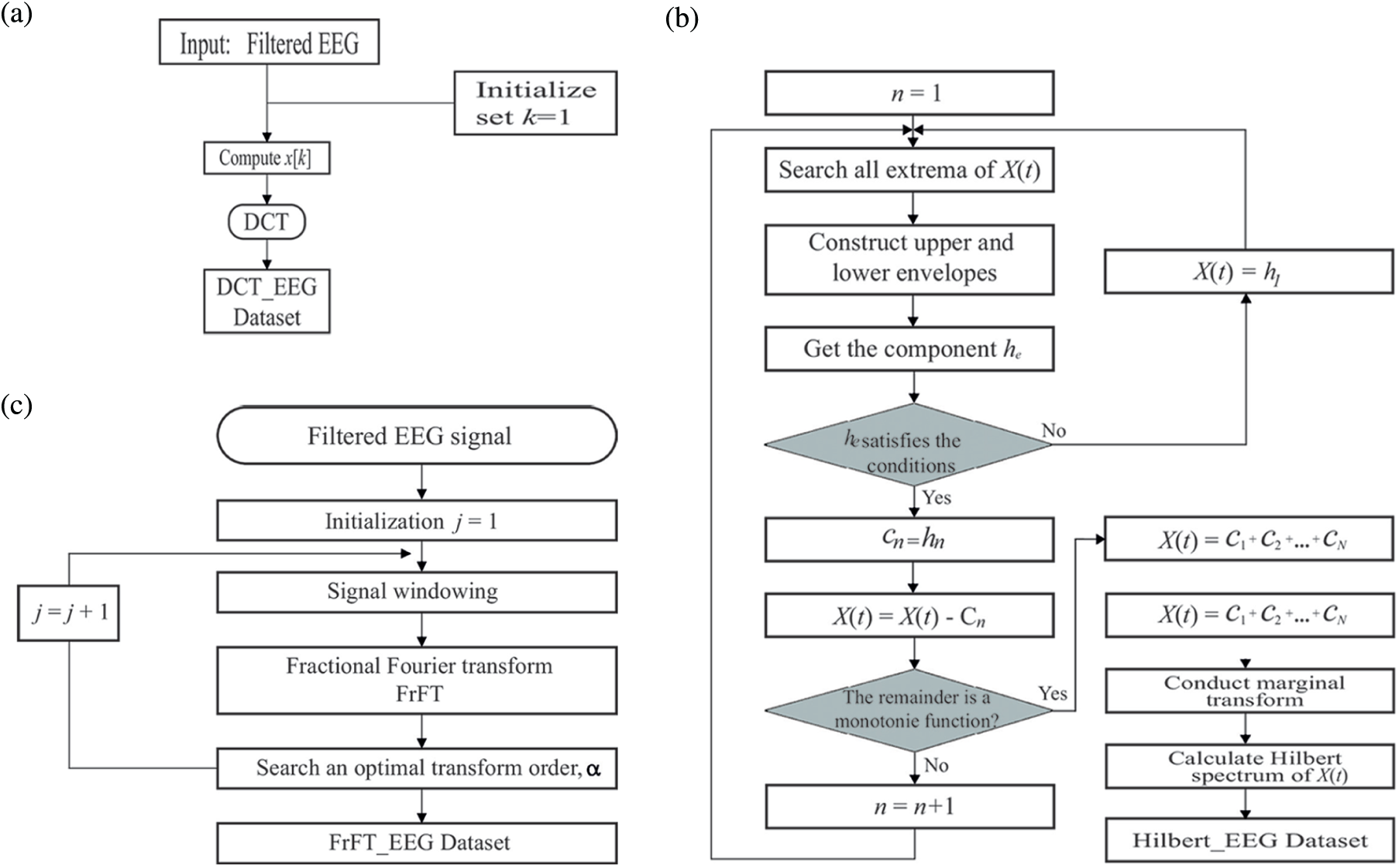
Figure 5: Flowchart of obtaining the DCT_EEG (a), FrFT_EEG (b), HT_EEG (c)

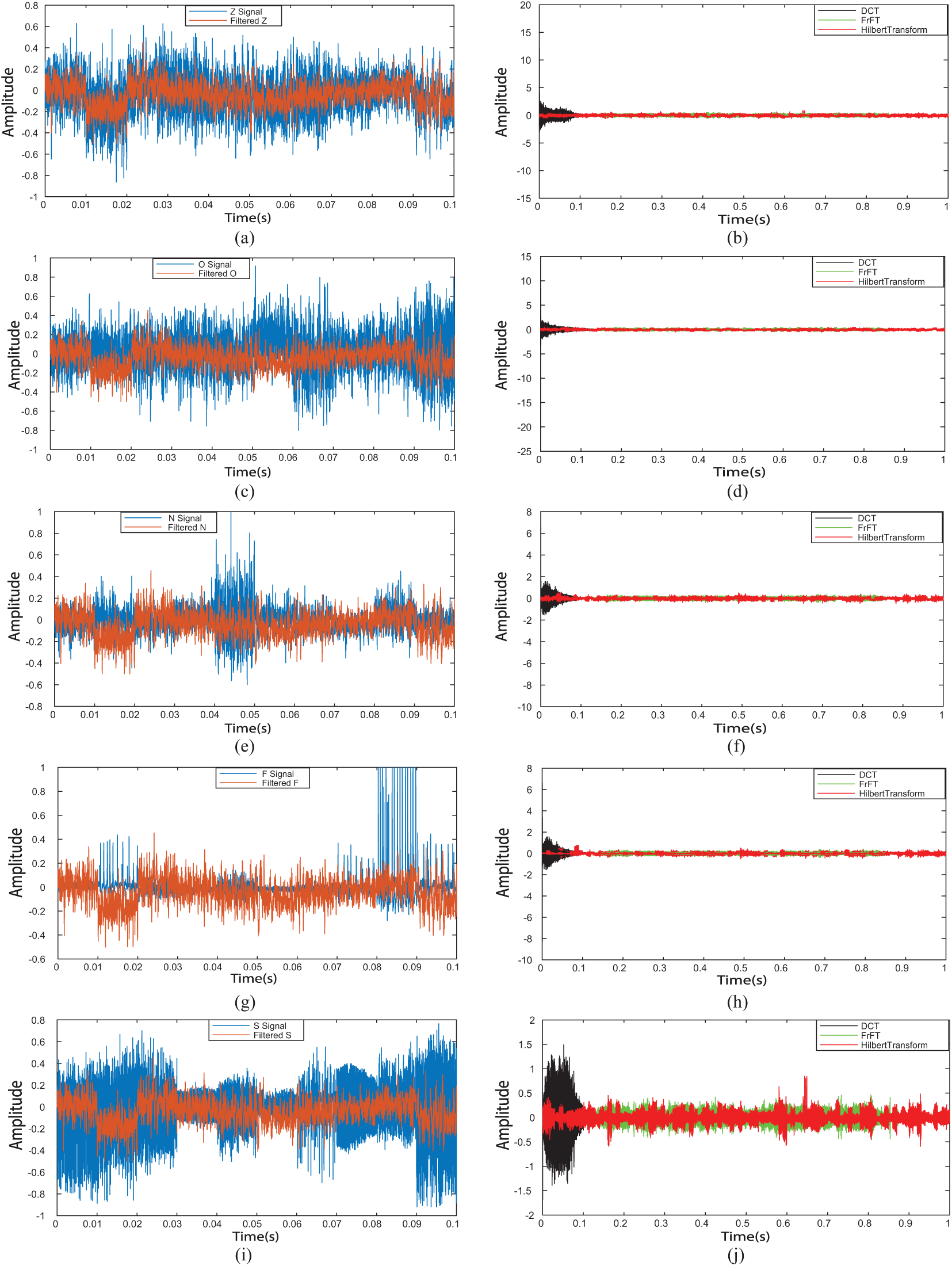
Figure 6: Filtered EEG signals and time frequency analysis EEG signals. (a) Filtered Z signal, (b) time-frequency analysis for Z signal, (c) filtered O signal, (d) time-frequency analysis for O signal, (e) filtered N signal, (f) time-frequency analysis for N signal, (g) filtered F signal, (h) time-frequency analysis for F signal, (i) filtered S signal, (j) time-frequency analysis for S signal

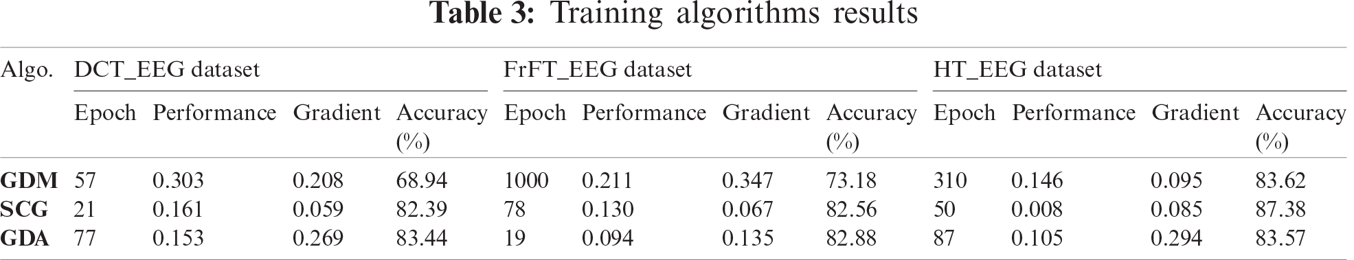
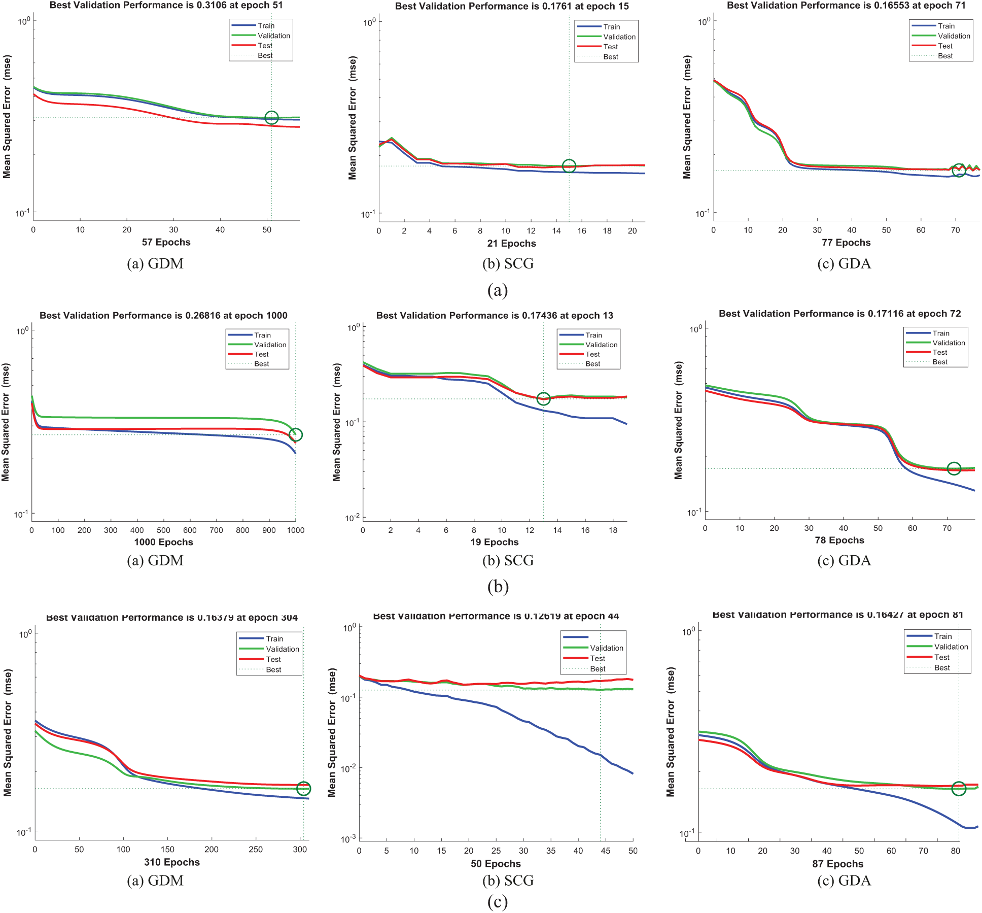
Figure 7: The classification performances of DCT_EEG, FrFT_EEG, HT_EEG datasets (a) DCT_EEG dataset classification performance (b) FrFT_EEG dataset classification performance (c) HT_EEG dataset classification performance

In this study, DCT_EEG, FrFT_EEG, and HT_EEG were obtained according to the following steps.

Step 1: DCT_EEG, FrFT_EEG, and HT_EEG datasets were obtained from the extracranial {Z, O} and the intracranial {N, F, S} EEG signals, which are shown in Figs. 6b, 6d, 6f, 6h and 6j by the black line, green line, and red line, respectively.

Step 2: Classification for the extracranial and the intracranial EEG signal datasets were trained by the ANN-BP training algorithms of GDM, SCG, and GDA. All the three training algorithms were stopped when any of the following conditions occurred: reaching the maximum number of epochs, exceeding the maximum duration, minimizing performance to the goal, and dropping below the minimum gradient.

Step 3: The options for the neural network architecture of the proposed GDM, SCG, and GDA training algorithms for choosing the right optimizer with the correct parameters are as follows: (i) Ten hidden layers were created with the sigmoid transfer function. (ii) The training epochs, (lr), minimum gradient, and the momentum coefficient were set at 1000, 0.01, 1e −05, and 0.5, respectively. (iii) The classification performances of all three algorithms were compared according to their mean squared error (mse) results. The outputs were EEG signals, specifically {Z, O, N, F, S}. DCT_EEG, FrFT_EEG, and HT_EEG datasets had the dimensions of (4097×500), and they had been randomly divided 70% for training, 15% for testing, and 15% for validation. All the ANN-BP training results for the training algorithm are shown in Tab. 3. The time-frequency method was HT. HT was the most successful significant signal feature descriptor for all three training algorithms in comparison with DCT and FrFT methods.

The training, test, and validation performance results of the algorithms are shown in Figs. 7a, 7b, and 7c. The validation performances were increased more than the maximum validation time since the last decrease during the experimental processes of this study.

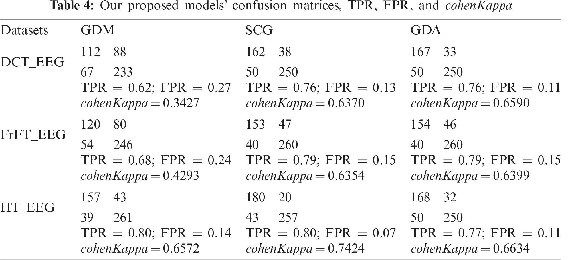
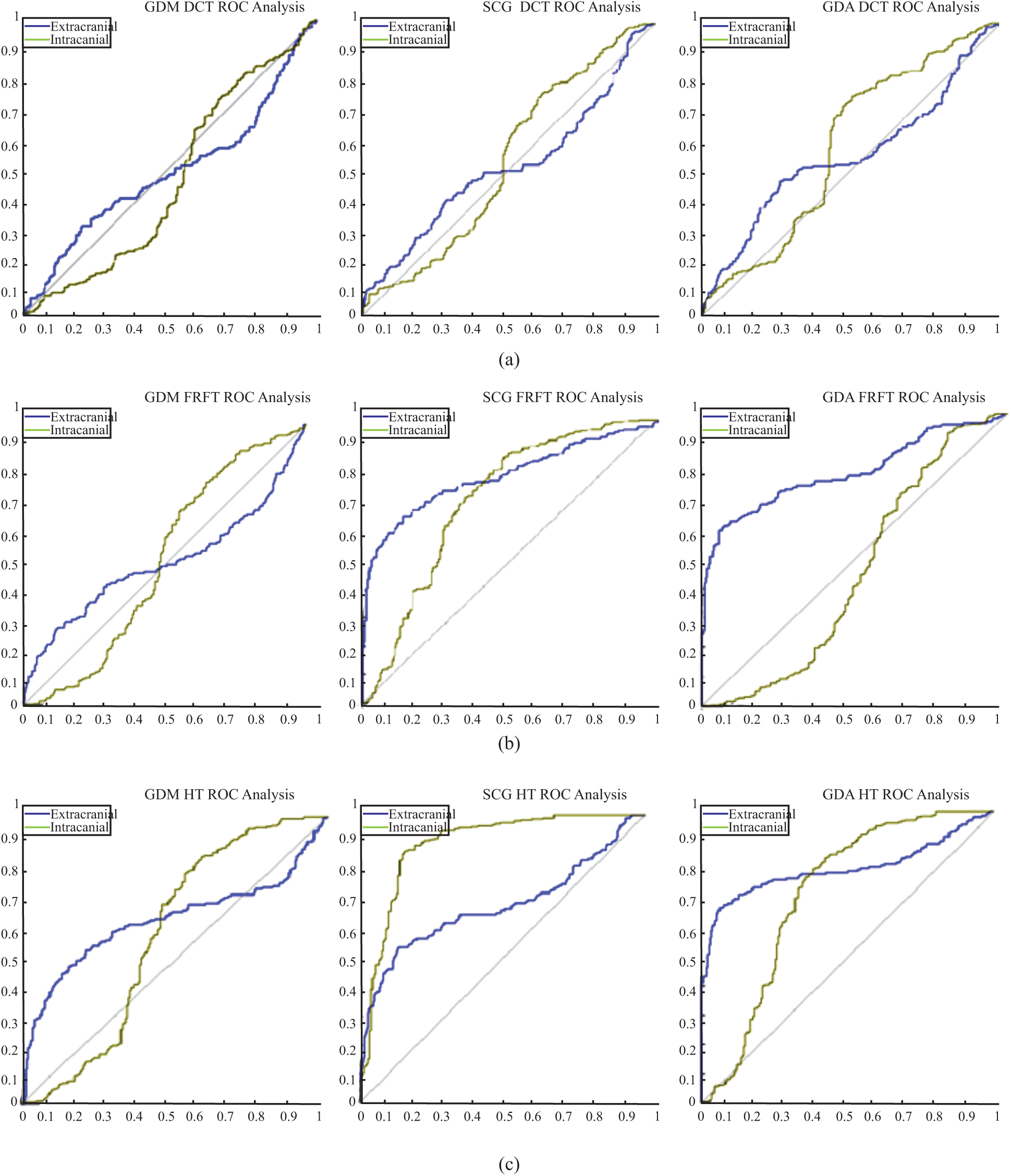
Figure 8: ROC analyses results (a) ROC analysis for the DCT_EEG dataset (b) ROC analysis for the FrFT_EEG dataset (c) ROC analysis for the HT_EEG dataset

3.1 Comparison with Other Work

The results of the proposed method were compared with other methods in the literature. In our study, the experimental results were compared with their classification accuracy rates and statistical analysis results. Hence, the proposed methods listed in Tab. 1 were used to test their performances for classifying {Z, O, N, F, S} or {A, B, C, D, E} signals. This study selects the distinct and significant features in Z, O (or AB) and N, F, S (or CDE) classification by time frequency methods as in earlier studies [25,31,43,46]. No other study has been found in the literature comparing datasets obtained from three time-frequency methods together. The popular ANN-BP algorithms were applied to the datasets comprising distinct and significant time-frequency domain features. Lastly, the points that distinguished our proposed models from other studies are as follows: (i) our model discovered a way to classify extracranial signals {Z, O} and intracranial signals {N, F, S}; (ii) different datasets were obtained by the time frequency methods DCT, FrFT, and HT; (iii) the proposed methods were compared with the ANN-BP algorithms; (iv) HT was shown to be a promising way for both EEG signal processing and classification. The proposed method had some limitations, and our experiments need to be analyzed carefully in this context. First, this study was cross-sectional in terms of the BONN database and the nature of the EEGs in the database. We assessed the respondent of the brain perception of the patient for the cases at a specific time. We had to work under certain conditions that were defined by the database we used.

3.2 Evaluation of the Analysis

The cohenKappa values according to the ANN-BP algorithms are shown in Tab. 4. For the DCT_EEG dataset, the classification agreement between the two classes was weakly compatible for the GDM algorithm. However, the GDA algorithm fit well into the classification agreement. For the FrFT_EEG dataset, the classification agreement between the two classes was moderate compliance for the GDM algorithm. Alternatively, SCG and GDA algorithms fit well into the classification agreement. The HT_EEG dataset fit well into the classification agreement for all three algorithms. The diagonal divided the ROC area. Points on the diagonal represented good classification results; bad results were represented by the points below the line. The confusion matrices, TPR, FPR, and cohenKappa for our proposed model are shown in Tab. 4. The predictions of the proposed model in this study resulted from 200 extracranial signals and 300 intracranial signals instances.

The plots of the nine confusion matrices mentioned earlier in the ROC curves are shown in Fig. 8. The result of method SCG for the HT_EEG dataset clearly showed the best prediction compared with other models and datasets. The result of GDA for the HT_EEG dataset lies on the diagonal line (gray line), and the accuracy of GDA is 83.57% as shown in Tab. 4.

4  Conclusion

In this study, a novel clinical decision support system was developed for the diagnosis of epilepsy using extracranial and intracranial EEG signals. The main contribution of this study is that it proposes a brand-new computer vision-based approach for the measurement of EEG signals in epileptic individuals. Significant features were extracted using the time-frequency methods of DCT, FrFT, and HT. The extracted features were fed into the GDM, SCG, and GDA training algorithms. HT gave the best classification accuracy rates compared with DCT and FrFT methods with values of 87.38%, 83.62%, and 83.57%, respectively, for the three algorithms. The most distinctive time-frequency features were obtained using the significant EEG signal properties obtained from HT when applied to the SCG training algorithm. In future work, various features can be used to extract more efficient epilepsy-related properties, and will be tested for effectiveness. In particular, it is planned to use fractal-related, wavelet-related, and entropy-related features. In addition, more EEG signals data will be used to re-validate the novel learning algorithms, and other advanced machine learning algorithms will be validated with the ANN-BP training algorithms.

Funding Statement: This study was supported by The Scientific Technological Research Council of Turkey (TÜBITAK) under the Project No. 118E682.

Conflicts of Interest: The authors declare that they have no conflicts of interest to report regarding the present study.

References

 1.  S. Supriya, S. Siuly and Y. Zhang, “Automatic epilepsy detection from EEG introducing a new edge weight method in the complex network,” Electronics Letters, vol. 52, no. 17, pp. 1430–1432, 2016. [Google Scholar]

 2.  H. Jiang, Z. Wang, R. Jiao and S. Jiang, “Picture-induced EEG signal classification based on CVC emotion recognition system,” Computers, Materials & Continua, vol. 65, no. 2, pp. 1453–1465, 2020. [Google Scholar]

 3.  E. N. G. E. L. Jerome Jr, “ILAE commission report: A proposed diagnostic scheme for people with epileptic seizures and with epilepsy: Report of the ILAE task force on classification and terminology,” Epilepsia: Journal of the International League Against Epilepsy, vol. 42, no. 6, pp. 796–803, 2001. [Google Scholar]

 4.  L. Hirsch and R. Brenner, EEG basics: In Atlas of EEG in Critical Care, 1st ed. Malaysia: John Wiley & Sons Press, pp. 1–54, 2010. [Google Scholar]

 5.  E. Kabir and Y. Zhang, “Epileptic seizure detection from EEG signals using logistic model trees,” Brain Informatics, vol. 3, no. 2, pp. 93–100, 2016. [Google Scholar]

 6.  R. San-Segundo, M. Gil-Martín, L. F. D’Haro-Enríquez and J. M. Pardo, “Classification of epileptic EEG recordings using signals transforms and convolutional neural networks,” Computers in Biology and Medicine, vol. 109, no. 4, pp. 148–158, 2019. [Google Scholar]

 7.  U. R. Acharya, S. V. Sree, A. P. C. Alvin and J. S. Suri, “Use of principal component analysis for automatic classification of epileptic EEG activities in wavelet framework,” Expert System with Applications, vol. 39, no. 10, pp. 9072–9078, 2012. [Google Scholar]

 8.  S. M. Alam and M. I. Bhuiyan, “Detection of seizure and epilepsy using higher order statistics in the EMD domain,” IEEE Journal Biomedical Health Information, vol. 17, no. 2, pp. 312–318, 2013. [Google Scholar]

 9.  H. U. Amin, M. Z. Yusoff and R. F. Ahmad, “A novel approach based on wavelet analysis and arithmetic coding for automated detection and diagnosis of epileptic seizure in EEG signals using machine learning techniques,” Biomedical Signal Processing and Control, vol. 56, no. 101707, pp. 1–10, 2020. [Google Scholar]

10. G. Chen, “Automatic EEG seizure detection using dual-tree complex wavelet-Fourier features,” Expert System with Applications, vol. 41, no. 5, pp. 2391–2394, 2014. [Google Scholar]

11. A. B. Das, M. I. H. Bhuiyan and S. M. S. Alam, “Classification of EEG signals using normal inverse Gaussian parameters in the dual-tree complex wavelet transform domain for seizure detection,” Signal Image and Video Processing, vol. 10, no. 2, pp. 259–266, 2016. [Google Scholar]

12. J. S. Saini and R. Dhiman, “Genetic algorithms tuned expert model for detection of epileptic seizures from EEG signatures,” Application Soft Computing, vol. 19, no. 2, pp. 8–17, 2014. [Google Scholar]

13. E. Fernandez-Blanco, D. Rivero, J. Rabuñal, J. Dorado, A. Pazos et al., “Automatic seizure detection based on star graph topological indices,” Journal Neuroscience Methods, vol. 209, no. 2, pp. 410–419, 2012. [Google Scholar]

14. L. Guo, D. Rivero, J. A. Seoane and A. Pazos, “Classification of EEG signals using relative wavelet energy and artificial neural networks,” in Proc. of the First ACM/SIGEVO Summit on Genetic and Evolutionary Computation, Shanghai, China, pp. 177–183, 2009. [Google Scholar]

15. L. Guo, D. Rivero, J. Dorado, J. R. Rabunal and A. Pazos, “Automatic epileptic seizure detection in EEGs based online length feature and artificial neural networks,” Journal Neuroscience Methods, vol. 191, no. 1, pp. 101–109, 2010. [Google Scholar]

16. L. Guo, D. Rivero and A. Pazos, “Epileptic seizure detection using multiwavelet transform based approximate entropy and artificial neural networks,” Journal Neuroscience Methods, vol. 193, no. 1, pp. 156–163, 2010. [Google Scholar]

17. V. Joshi, R. B. Pachori and A. Vijesh, “Classification of ictal and seizure-free EEG signals using fractional linear prediction,” Biomedical Signal Processing Control, vol. 9, no. 5, pp. 1–5, 2014. [Google Scholar]

18. J. H. Kang, Y. G. Chung and S. P. Kim, “An efficient detection of epileptic seizure by differentiation and spectral analysis of electroencephalograms,” Computers in Biology and Medicine, vol. 66, pp. 352–356, 2015. [Google Scholar]

19. N. Kannathal, U. R. Acharya, C. M. Lim and P. K. Sadasivan, “Characterization of EEG: A comparative study,” Computer Methods and Programs in Biomedicine, vol. 80, no. 1, pp. 17–23, 2005. [Google Scholar]

20. N. Kannathal, M. L. Choo, U. R. Acharya and P. K. Sadasivan, “Entropies for detection of epilepsy in EEG,” Computer Methods and Programs in Biomedicine, vol. 80, no. 3, pp. 187–194, 2005. [Google Scholar]

21. Y. Kaya, M. Uyar, R. Tekin and S. Yıldırım, “1D-local binary pattern-based feature extraction for classification of epileptic EEG signals,” Applied Mathematics and Computation, vol. 243, no. 6, pp. 209–219, 2014. [Google Scholar]

22. Y. Kumar, M. L. Dewal and R. S. Anand, “Epileptic seizures detection in EEG using DWT-based ApEn and artificial neural network,” Signal Image and Video Processing, vol. 8, no. 7, pp. 1323–1334, 2014. [Google Scholar]

23. T. S. Kumar, V. Kanhangad and R. B. Pachori, “Classification of seizure and seizure-freeEEG signals using local binary patterns,” Biomedical Signal Processing and Control, vol. 15, no. 9, pp. 33–40, 2015. [Google Scholar]

24. S. H. Lee, J. S. Lim, J. K. Kim, J. Yang and Y. Lee, “Classification of normal and epileptic seizure EEG signals using wavelet transform, phase-space reconstruction, and Euclidean distance,” Computer Methods and Programs in Biomedicine, vol. 116, no. 1, pp. 10–25, 2014. [Google Scholar]

25. M. Li, W. Chen and T. Zhang, “Application of MODWT and log-normal distribution model for automatic epilepsy identification,” Biocybernetics and Biomedical Engineering, vol. 37, no. 4, pp. 679–689, 2017. [Google Scholar]

26. S. F. Liang, H. C. Wang and W. L. Chang, “Combination of EEG complexity and spectral analysis for epilepsy diagnosis and seizure detection,” EURASIP Journal on Advances in Signal Processing, vol. 1, pp. 1–15, 2010. [Google Scholar]

27. J. Martinez-del-Rincon, M. J. Santofimia, X. Toro, J. Barba, F. Romero et al., “Non-linear classifiers applied to EEG analysis for epilepsy seizure detection,” Expert Systems with Applications, vol. 86, no. 4, pp. 99–112, 2017. [Google Scholar]

28. M. Mursalin, Y. Zhang, Y. Chen and N. V. Chawla, “Automated epileptic seizure detection using improved correlation-based feature selection with random forest classifier,” Neurocomputing, vol. 241, no. 10, pp. 204–214, 2017. [Google Scholar]

29. A. S. M. Murugavel and S. Ramakrishnan, “Hierarchical multi-class SVM with ELM kernel for epileptic EEG signal classification,” Medical & Biological Engineering & Computing, vol. 54, no. 1, pp. 149–161, 2016. [Google Scholar]

30. N. Nicolaou and J. Georgiou, “Detection of epileptic electroencephalogram based on permutation entropy and support vector machines,” Expert Systems with Applications, vol. 39, no. 1, pp. 202–209, 2012. [Google Scholar]

31. U. Orhan, M. Hekim and M. Ozer, “EEG signals classification using the k-means clustering and a multilayer perceptron neural network model,” Expert Systems with Applications, vol. 38, no. 10, pp. 13475–13481, 2011. [Google Scholar]

32. M. Peker, B. Sen and D. Delen, “A novel method for automated diagnosis of epilepsy using complex-valued classifiers,” IEEE Journal of Biomedical and Health Informatics, vol. 20, no. 1, pp. 108–118, 2016. [Google Scholar]

33. K. Polat and S. Gunes, “Classification of epileptiform EEG using a hybrid system based on decision tree classifier and fast Fourier transform,” Applied Mathematics and Computation, vol. 187, no. 2, pp. 1017–1026, 2007. [Google Scholar]

34. K. Samiee, P. Kovács and M. Gabbouj, “Epileptic seizure classification of EEG time-series using rational discrete short-time Fourier transform,” IEEE Transactions on Biomedical Engineering, vol. 62, no. 2, pp. 541–552, 2015. [Google Scholar]

35. M. Sharma, R. B. Pachori and U. R. Acharya, “A new approach to characterize epileptic seizures using analytic time-frequency flexible wavelet transform and fractal dimension,” Pattern Recognition Letters, vol. 94, no. 7, pp. 172–179, 2017. [Google Scholar]

36. L. Y. Siuly and P. Wen, “Clustering technique-based least square support vector machine for EEG signal classification,” Computer Methods and Programs in Biomedicine, vol. 104, no. 3, pp. 358–372, 2011. [Google Scholar]

37. V. Srinivasan, C. Eswaran and N. Sriraam, “Approximate entropy-based epileptic EEG detection using artificial neural networks,” IEEE Transactions on Information Technology in Biomedicine, vol. 11, no. 3, pp. 288–295, 2007. [Google Scholar]

38. N. S. Tawfik, S. M. Youssef and M. Kholief, “A hybrid automated detection of epileptic seizures in EEG records,” Computers & Electrical Engineering, vol. 53, no. 7, pp. 177–190, 2016. [Google Scholar]

39. A. K. Tiwari, R. B. Pachori, V. Kanhangad and B. K. Panigrahi, “Automated diagnosis of epilepsy using key-point-based local binary pattern of EEG signals,” IEEE Journal of Biomedical and Health Informatics, vol. 21, no. 4, pp. 888–896, 2017. [Google Scholar]

40. M. G. Tsipouras, “Spectral information of EEG signals with respect to epilepsy classification,” EURASIP Journal on Advances in Signal Processing, vol. 10, pp. 1–17, 2019. [Google Scholar]

41. A. T. Tzallas, M. G. Tsipouras and D. I. Fotiadis, “Automatic seizure detection based on time-frequency analysis and artificial neural networks,” Computational Intelligence and Neuroscience, vol. 2007, no. 4, pp. 1–13, 2007. [Google Scholar]

42. A. T. Tzallas, M. G. Tsipouras and D. I. Fotiadis, “Epileptic seizure detection in EEGs using time-frequency analysis,” IEEE Transactions on Information Technology in Biomedicine, vol. 13, no. 5, pp. 703–710, 2009. [Google Scholar]

43. I. Ullah, M. Hussain, E. U. H. Qazi and H. Aboalsamh, “An automated system for epilepsy detection using EEG brain signals based on deep learning approach,” Expert Systems with Applications, vol. 107, no. 4, pp. 61–71, 2018. [Google Scholar]

44. X. Wang, G. Gong and N. Li, “Automated recognition of epileptic EEG States using a combination of symlet wavelet processing, gradient boosting machine, and grid search optimizer,” Sensors, vol. 19, no. 219, pp. 1–18, 2019. [Google Scholar]

45. S. Xie and S. Krishnan, “Wavelet-based sparse functional linear model with applications to EEGs seizure detection and epilepsy diagnosis,” Medical & Biological Engineering & Computing, vol. 51, no. 1–2, pp. 49–60, 2013. [Google Scholar]

46. T. Zhang, W. Chen and M. Li, “Fuzzy distribution entropy and its application in automated seizure detection technique,” Biomedical Signal Processing and Control, vol. 39, no. 12, pp. 360–377, 2018. [Google Scholar]

47. G. Zhu, Y. Li and P. P. Wen, “Epileptic seizure detection in EEGs signals using a fast weighted horizontal visibility algorithm,” Computer Methods and Programs in Biomedicine, vol. 115, no. 2, pp. 64–75, 2014. [Google Scholar]

48. P. Swami, T. K. Gandhi, B. K. Panigrahi, M. Tripathi and S. Anand, “A novel robust diagnostic model to detect seizures in electroencephalography,” Expert Systems with Applications, vol. 56, pp. 116–130, 2016. [Google Scholar]

49. R. G. Andrzejak, K. Lehnertz, F. Mormann, C. Rieke, P. David et al., “Indications of nonlinear deterministic and finite-dimensional structures in time series of brain electrical activity: Dependence on recording region and brain state,” Physical Review E, vol. 64, no. 6, pp. 061907, 2001. [Google Scholar]

50. F. Taylor, Finite Impulse Response Filters in Digital Filters Principles and Applications with MATLAB, 1st ed. Canada: John Wiley & Sons Press, pp. 53–70, 2011. [Google Scholar]

51. L. Jing, L. Jingbing, C. Jieren, M. Jixin, S. Naveed et al., “A novel robust watermarking algorithm for encrypted medical image based on DTCWT-DCT and chaotic map,” Computers, Materials & Continua, vol. 61, no. 2, pp. 889–910, 2019. [Google Scholar]

52. Z. Wang, Q. Wang, J. Liu, Z. Liang and J. Xu, “New SARimaging algorithm via the optimal time-frequency transform domain,” Computers, Materials & Continua, vol. 65, no. 3, pp. 2351–2363, 2020. [Google Scholar]

53. A. Bhattacharyya, V. Gupta and R. B. Pachori, “Automated identification of epileptic seizure EEG signals using empirical wavelet transform based Hilbert marginal spectrum,” in Proc. of the Twenty Second Int. Conf. on Digital Signals Processing, London, UK, pp. 1–5, 2017. [Google Scholar]

54. S. Bayrak, E. Yucel and H. Takci, “Classification of extracranial and intracranial EEG signals by using finite impulse response filter through ensemble learning,” in Proc. of the Twenty Seventh Signals Processing and Communications Applications Conf., Sivas, Turkey, pp. 1–4, 2019. [Google Scholar]

55. C. Anitescu, E. Atroshchenko, N. Alajlan and T. Rabczuk, “Artificial neural network methods for the solution of second order boundary value problems,” Computers, Materials & Continua, vol. 59, no. 1, pp. 345–359, 2019. [Google Scholar]

56. S. Ruder, “An overview of gradient descent optimization algorithms,” arXiv preprint arXiv: 1609.04747, 2016. [Google Scholar]

57. M. F. Møller, “A scaled conjugate gradient algorithm for fast supervised learning,” Neural Networks, vol. 6, no. 4, pp. 525–533, 1993. [Google Scholar]

58. R. Battiti, “First-and second-order methods for learning: Between steepest descent and Newton’s method,” Neural Computation, vol. 4, no. 2, pp. 141–166, 1992. [Google Scholar]

59. J. R. Landis and G. G. Koch, “An application of hierarchical kappa-type statistics in the assessment of majority agreement among multiple observers,” Biometrics, vol. 33, no. 2, pp. 363–374, 1977. [Google Scholar]

60. T. Fawcett, “An introduction to ROC analysis,” Pattern Recognition Letters, vol. 27, no. 8, pp. 861–874, 2006. [Google Scholar]

This work is licensed under a Creative Commons Attribution 4.0 International License, which permits unrestricted use, distribution, and reproduction in any medium, provided the original work is properly cited.