Computers, Materials & Continua DOI:10.32604/cmc.2021.018320
Article

Support Vector Machine Assisted GPS Navigation in Limited Satellite Visibility

Dah-Jing Jwo*, Jia-Chyi Wu and Kuan-Lin Ho

Department of Communications, Navigation and Control Engineering, National Taiwan Ocean University, Keelung, 202301, Taiwan
*Corresponding Author: Dah-Jing Jwo. Email: djjwo@mail.ntou.edu.tw
Received: 02 March 2021; Accepted: 04 April 2021

Abstract: This paper investigates performance improvement via the incorporation of the support vector machine (SVM) into the vector tracking loop (VTL) for the Global Positioning System (GPS) in limited satellite visibility. Unlike the traditional scalar tracking loop (STL), the tracking and navigation modules in the VTL are not independent anymore since the user’s position can be determined by using the information from other satellites and can be predicted on the basis of the states of the user. The method proposed in this paper makes use of the SVM to bridge the GPS signal and prevent the error growth due to signal outage. Similar to the neural network, the SVM is motivated by its ability to approximate an unknown nonlinear input-output mapping through supervised training. The SVM is employed for predicting adequate numerical control oscillator (NCO) inputs, i.e., providing better prediction of residuals for the Doppler frequency and code phase in order to maintain regular operation of the navigation system. When the navigation processing is in good condition, the SVM is at the training stage, and the output information from the discriminator and navigation filter is adopted as the inputs. Other machine learning (ML) algorithms such as the radial basis function neural network (RBFNN) and the Adaptive Network-Based Fuzzy Inference System (ANFIS) are employed for comparison. Performance evaluation for the SVM assisted architecture as compared to the RBFNN- and ANFIS-assisted methods and the un-assisted VTL will be carried out and the performance evaluation during GPS signal outage will be presented. The proposed design is very useful for navigation during the environment of limited satellite visibility to effectively overcome the problem in the environment of GPS outage.

Keywords: Global positioning system; support vector machine; machine learning; vector tracking loop; signal outage

1  Introduction

The Global Positioning System (GPS) is a satellite-based navigation system [1,2] that provides a user with the proper equipment access to useful and accurate positioning information anywhere on the globe. Generally, the GPS receiver accomplishes the following two major functions: the tracking of pseudo-range and the solution of navigation information. The signal tracking tries to adjust the local signal to have the same code phase with the received satellite signal. Traditional GPS receivers track signals from different satellites independently. Each tracking channel measures the pseudo-range and pseudo-range rate, respectively, and then sends the measurements to the navigation processor, which solves for the user’s position, velocity, clock bias and clock drift (PVT). Blockage and reflections from buildings and other large, solid objects can lead to GPS accuracy problems. Recently, several researchers have studied a vector tracking loop (VTL) [3–11], such as a vector delay lock loop (VDLL) and a vector frequency lock loop (VFLL), and the combination of both, called VDFLL, to obtain an improved tracking performance in the GPS receiver. Vector tracking loops integrate the tracking loops and navigation processor, such that each tracking loop update is also based on information from other tracking loops. For the vector tracking loop GPS, the tasks of signal tracking and navigation state estimation are no longer separate processes. The vector tracking loop architectures provide several important advantages as compared to the scalar tracking loops. One of the merits is that the tracking loop can be assisted positioning when satellite signal outage.

In the last years, the field of machine learning (ML) is expanding and many new technologies are growing using these principles. The first applications of ML have been related to data mining, text categorization, and pattern/facial recognition. This new learning algorithm can be seen as an alternative training technique for polynomial, radial basis function and multi-layer perceptron (MLP) classifiers. The neural networks (NNs) [11–14] have been studied since Rosenblatt first applied the single-layer perceptron to pattern classification learning in the late 1950s. They are trainable, dynamic systems that can estimate input-output functions and have been applied to a wide variety of problems since they are model-free estimators, i.e., without a mathematical model. An NN is a network structure consisting of a number of nodes connected through directional links. The importance of a NN includes the way a neuron is implemented and how their interconnection/topology is made.

Unlike the MLP networks, the radial basis function neural network (RBFNN) [11,15,16] has simple architecture of only three layers: input, hidden and output layers. In an RBFNN, only a single layer of nodes with radically symmetric basis activation functions is needed to achieve a smooth approximation to an arbitrary real nonlinear function. An adaptive neuro-fuzzy inference system or adaptive network-based fuzzy inference system (ANFIS) [15–20] is a kind of artificial neural network that is based on Takagi-Sugeno fuzzy inference system. As a combination of the Takagi-Sugeno fuzzy inference and neural network, the ANFIS can construct an input-output mapping based on both human knowledge (in the form of fuzzy if-then rules) and stipulated input-output data pairs. The purpose is to approximate unknown function or nonlinear input-output mapping through supervised training. They have been applied to wide variety of problems, for instance, approximate unknown function, the classification, the grade estimation, the design of the control system, since they are model-free estimator, i.e., without a mathematical model.

Since the 1990s there has been a significant activity in the theoretical development and applications of Support Vector Machine (SVM) [21–25], which is a supervised learning model that divides the data into regions separated by a linear boundary that divides the different features. Among the various existing algorithms, the so-called SVM is one of the most recognized for classification and regression that permit the creation of systems which, after training from a series of examples, can successfully predict the output at an unseen location performing an operation known as induction. The paper makes use of the SVM to bridge the GPS signal and prevent the error growth due to signal outage and the results will be compared with the RBFNN- and ANFIS- based methods [11].

The remainder of this paper is organized as follows. In Section 2, preliminary background on GPS navigation filter with vector tracking architecture is reviewed. The machine learning algorithms is briefly reviewed in Section 3. The system model for GPS vector tracking loop assisted by machine learning module is introduced in Section 4. In Section 5, illustrative examples are presented to evaluation of the effectiveness and for performance comparison due to various ML algorithms. Conclusions are given in Section 6.

2  GPS Navigation Filter with Vector Tracking Architecture

The traditional scalar tracking loop (STL) processes signals from each satellite separately. Specifically, a delay lock loop (DLL) is used to track the code phase of the incoming pseudorandom code and a carrier tracking loop, such as a frequency lock loop (FLL) or a phase lock loop (PLL), is used to track the carrier frequency or phase. The tracking results from different channels are then combined to estimate the navigation solutions. The drawback of STL is that it neglects the inherent relationship between the navigation solutions and the tracking loop status. In that sense, a STL is more like an open loop system and provides poor performance when scintillation, interference, or signal outages occur.

The vector tracking loop (VTL) provides a deep level of integration between signal tracking and navigation solutions in a GNSS receiver and results in several important improvements over the traditional STL such as increased interference immunity, robust dynamic performance, and the ability to operate at low signal power and bridge short signal outages. The architecture of the vector tracking loop (VTL) can be different depending on its implementation. The tracking input is not directly connected to the tracking control input rather the discriminator output is used in estimating pseudoranges. The extended Kalman filter (EKF) [26] in turn predicts the code phases. In VTL all channels are processed together in one processor which is typically an EKF. Therefore, even if the signals from some satellites are very weak the receiver can track them from the navigation results of the other satellite. VTL is a very attractive technique as it can provide tracking capability in degraded signal environment. Fig. 1 shows the system architectures for scalar tracking loop and vector tracking loop.

The conventional VTL based on the discriminator consists of correlator, discriminator and NCO. The loop filter is removed in each channel. The VTL discriminator outputs of each channel are passed to the navigation filter. These are used as the measurement of the navigation filter. The Doppler frequency and the pseudoranges are calculated from the estimated user position and velocity of the navigation filter. In general, it is known that the VTL based on the discriminator gives users an accurate position and Doppler frequency than the scalar vector tracking loop. The VTL based on the discriminator cannot deal with several problems, such as a rejection of channel with a low quality signal, high dynamic situation and others. The system architecture of the VTL is shown as in Fig. 1. The integrity check algorithms are used to detect the possible error in each channel to prevent the spreading of the error.

The EKF is used for estimation of the navigation states in GPS receivers. The process model and measurement model for the EKF can be written as

where the state vector xk∈ℜn, process noise vector wk∈ℜn, measurement vector zk∈ℜm, and measurement noise vector vk∈ℜm. Both the vectors wk and vk are zero mean Gaussian white sequences having zero crosscorrelation with each other:

where E[⋅] represents expectation, and superscript “T” denotes matrix transpose, Qk is the process noise covariance matrix, Rk is the measurement noise covariance matrix.

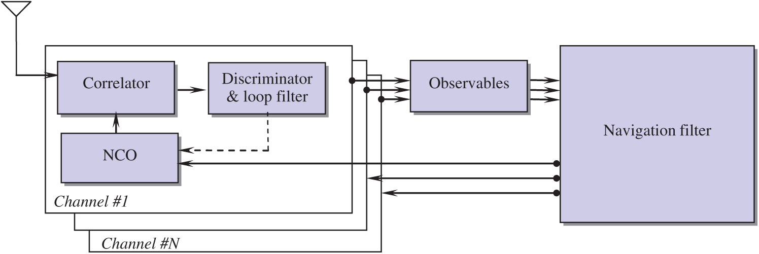
Figure 1: The system architecture of a vector tracking loop

The discrete-time extended Kalman filter algorithm is summarized as follow:

•   Correction steps/measurement update equations:

Kk=Pk−HkT[HkPk−HkT+Rk]−1(1)

x^k=x^k−+Kk[zk−hk(x^k−)](2)

Pk=[I−KkHk]Pk−(3)

•   Prediction steps/time update equations:

x^k+1−=fk(x^k)(4)

Pk+1−=ΦkPkΦkT+Qk(5)

The Kalman filter algorithm starts with an initial condition value, x^0− and P0−. When new measurement zk becomes available with the progression of time, the estimation of states and the corresponding error covariance would follow recursively ad infinity. The linear approximation equations for system and measurement matrices are obtained through the relations

Φk≈∂fk∂xk|xk=x^k−;Hk≈∂hk∂xk|xk=x^k−(6)

Further detailed discussion can be referred to Brown et al. [26].

3  Machine Learning Algorithms

In this section, three machine learning algorithms adopted in this paper are briefly reviewed, including the RBFNN, ANFIS and SVM. The RBFNN has simple architecture of only three layers: input, hidden and output layers. The ANFIS is a combination of the Sugeno fuzzy inference and neural network to approximate unknown function or nonlinear input-output mapping through supervised training. A SVM is a supervised learning model that divides the data into regions separated by a boundary that divides the different features.

3.1 The Radial Basis Function Neural Network

The RBFNN possesses an equivalent structure to the so-called optimal Bayesian equalization solution, and it can provide the conditional density function (CODF) of the transmitted symbols. Fig. 2 shows the architecture of a typical RBFNN. The overall response of the RBF network F(x) using Gaussian function φj(x) can be formulated as

F(x)=∑j=1Jwjφj(x)+b=∑j=0Jwjφj(x)(7)

and

ϕj(x)=exp⁡(−‖x−mj‖22σj2)(8)

where x is the input pattern; mj=1,…,N represents the centers of the RBF network, which have the same dimensionality as the input vector ; ‖⋅‖ denotes the Euclidean norm; ϕj(·) is the Gaussian (basis) function of the j-th neuron; σ is a positive constant representing the width of the RBF; wj is the weight of the RBF network; and b is the bias; p is the number of inputs; J is the number of neurons in the hidden layer (also the number of centers for the RBF).

[1φ1(x1)⋯φJ(x1)1φ1(x2)⋮⋮⋮⋱⋮1φ1(xN)⋯φJ(xN)]N×(J+1)[bw1⋮wJ](J+1)×1=[d1d2⋮dN]N×1(9)

where N is the number of training pattern. The above equation can be written in the simplified form

ΦW=d(10)

The weigh vector W is calculated by the pseudoinverse matrix method

W=(ΦTΦ)−1ΦTd(11)

And the output of the RBF network is given by

F(x)=∑j=1JWj⋅φj(12)

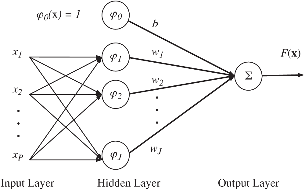
Figure 2: Architecture of a radial basis function neural network (RBFNN)

3.2 The Adaptive Network-based Fuzzy Inference System

Proposed by Jang in 1993 [15], the adaptive network-based fuzzy inference system (ANFIS) is a multilayer feed-forward network where each node performs a particular node function on incoming signals, in which Takagi and Sugeno’s type fuzzy inference is employed. The ANFIS employed in the present work has the architecture as shown in Fig. 3, which is composed of five layers given as follows:

Layer 1: Calculate membership value for premise parameter

O1i=μAi(x)for i=1,2;O1i=μBi−2(y)for i=3,4;(13)

μAi(x) and μBi−2(y): any appropriate parameterized membership functions.

O1i: the membership grade of a fuzzy set and it specifies the degree to which the given input x(y) satisfies the quantifier A.

Layer 2: Firing strength of rule

O2i=μAi(x)∗μBi(y)i=1,2(14)

Each node output represents the firing strength of a fuzzy control rule.

Layer 3: Normalize firing strength

O3i=w¯i=wiw1+w2for i=1,2(15)

Outputs of this layer are called normalized firing strengths.

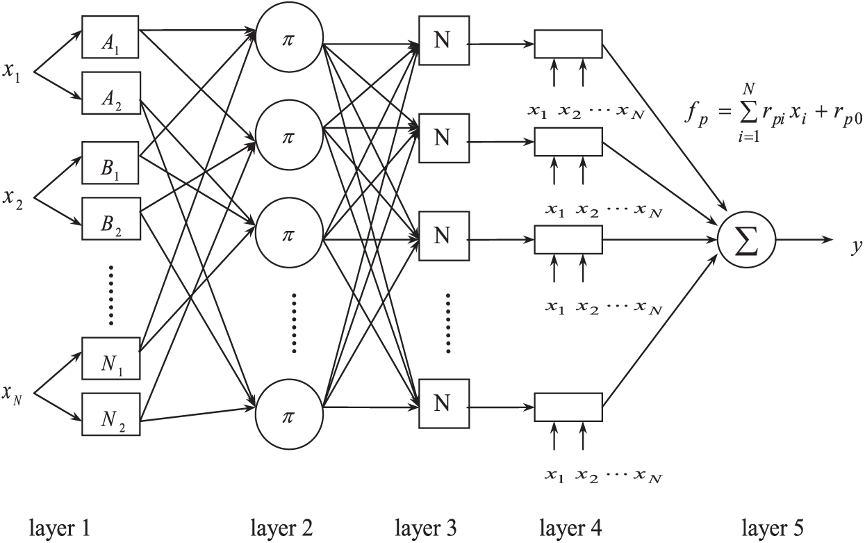
Figure 3: The adaptive network-based fuzzy inference system (ANFIS) architecture

Layer 4: Consequent parameters

O4i=w¯ifi=w¯i(pix+qiy+ri)(16)

Layer 5: Overall output

O5i=∑iw¯ifi=w¯1f1+w¯2f2(17)

3.3 The Support Vector Machine

A support vector machine is a supervised learning model that divides the data into regions separated by a boundary. There are two approaches for the SVM optimization, the linear and the non-linear kernels, depending on the nature of the problem. The main idea behind the technique is to separate the classes with a surface that maximizes the margin between them. They map the input (x) into a high-dimensional feature space (z=ϕ(x)) and construct an optimal decision boundary called the separating hyperplane. In general, SVMs find a classification function that separates data classes, with the largest margin, using a hyperplane. The principal difference between all machine learning algorithms regardless of the application, is the mathematical operation involved in calculating the optimal separating hyperplane. Fig. 4 shows a binary classification example of linear SVM. The linear boundary here divides the red triangles from the blue circles. If the training data is linearly separable, two parallel hyperplanes can be selected that separate the two classes of data, so that the distance between them is as large as possible. The region bounded by these two hyperplanes is called the margin, and the maximum-margin hyperplane is the hyperplane that lies halfway between them. The samples/data points on the margin are called support vectors.

A hyperplane can be written as the set of points x satisfying wTx−b=0, where w is the (not necessarily normalized) normal vector to the hyperplane. The parameter b/‖w‖ determines the offset of the hyperplane from the origin along the normal vector w. With a normalized or standardized dataset, these hyperplanes can be described by the equations wTx−b=1 (anything on or above this boundary is of one class, with label 1) and wTx−b=−1 (anything on or below this boundary is of the other class, with label −1). Geometrically, the distance between these two hyperplanes is 2/‖w‖ so to maximize the distance between the planes we want to minimize ‖w‖.

For SVMs with L1 soft-margin formulation, this is done by solving the primal problem:

minw,b,ξ12‖w‖2+12C∑i=1Nξi(18)

subject to

The parameter C is a penalty factor to control the trade-off between training error and generalization ability and its value is chosen by means of a validation set. The problem of the Lagrange dual form is:

max∑i=1Nαi−12∑i,j=1Nαiαjyiyjk(xi,xj)(19)

with constraints

where k(xi,xj)=φ(xi), in which φ(xj) is a kernel function of the nonlinear mapping implementation. A number of commonly used kernel functions include: linear, Gaussian, polynomial, RBF, and sigmoid kernels. To obtain a good performance, some parameters in SVMs have to be chosen carefully. These parameters include the regularization parameter C, which determines the trade-off between minimizing the training error and minimizing model complexity and parameter (d, σ or γ) of the kernel function.

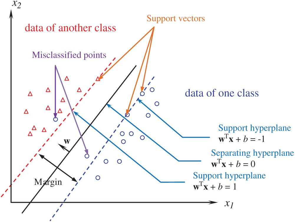
Figure 4: A binary classification example of linear support vector machine (SVM)

4  Vector Tracking Loop Assisted by Machine Learning Module

When selecting extended Kalman filtering as the navigation state estimator in the GPS receiver, using b and d to represent the GPS receiver clock bias and drift, the differential equation for the clock error is written as b˙=d+ub and d˙=ud, where ub∼N(0,Sf) and ud∼N(0,Sg) are independent Gaussianly distributed white sequences. The dynamic process of the GPS receiver in lower dynamic environment can be represented by the PV (Position-Velocity) model. In such case, we consider the GPS navigation filter with three position states, three velocity states, and two clock states, so that the state to be estimated is a 8×1 vector. The process model is assumed to be linear given by

where x1, x3, x5 represent the east, north, and vertical position; x2, x4, x6 represent the east, north, and vertical velocity; x7 and x8 represent the receiver clock offset and drift errors, respectively. The process noise covariance matrix is as follows:

Qk=[QeQnQuQt](20)

where

If only the pseudorange observables are available, the linearized measurement equation based on n observables can be written as

[ρ1ρ2⋮ρn]−[ρ^1ρ^2⋮ρ^n]⏟Zk=[hx(1)0hy(1)0hz(1)010hx(2)0hy(2)0hz(2)010⋮⋮⋮⋮⋮⋮⋮⋮hx(n)0hy(n)0hz(n)010]⏟Hk[x1x2x3x4x5x6x7x8]+[vρ1vρ2⋮vρn](21)

where (hx,ihy,ihz,i) is the line-of-sight unit vector, (x^uy^uz^u) represent the user position and (xiyizi) represent the satellite position. If the measurement equation for the navigation filter is composed of pseudorange and range-rate observables, the measurement matrix Hk is an (n×8) matrix

In order to further improve the tracking performance in degraded signal environment, the machine learning mechanism is used to aid the Kalman filter in the application of tracking loop design. Fig. 5a provides the ML assisted vector tracking loop for the environment of signal outage. The innovation can be written as

υk=zk−z^k−=zk−hk(x^k−)(22)

The trace of innovation covariance matrix can be obtained through the relation: υkTυk=tr(υkυkT). When the signal is in good condition, the ML is in the training stage, where the input data employed for the training stage is ε given by

εk=υkTυkm(23)

at the current and past 100 time epochs. The output is the υk at the next time epoch. The training procedure for the ML is shown as in Fig. 5b.

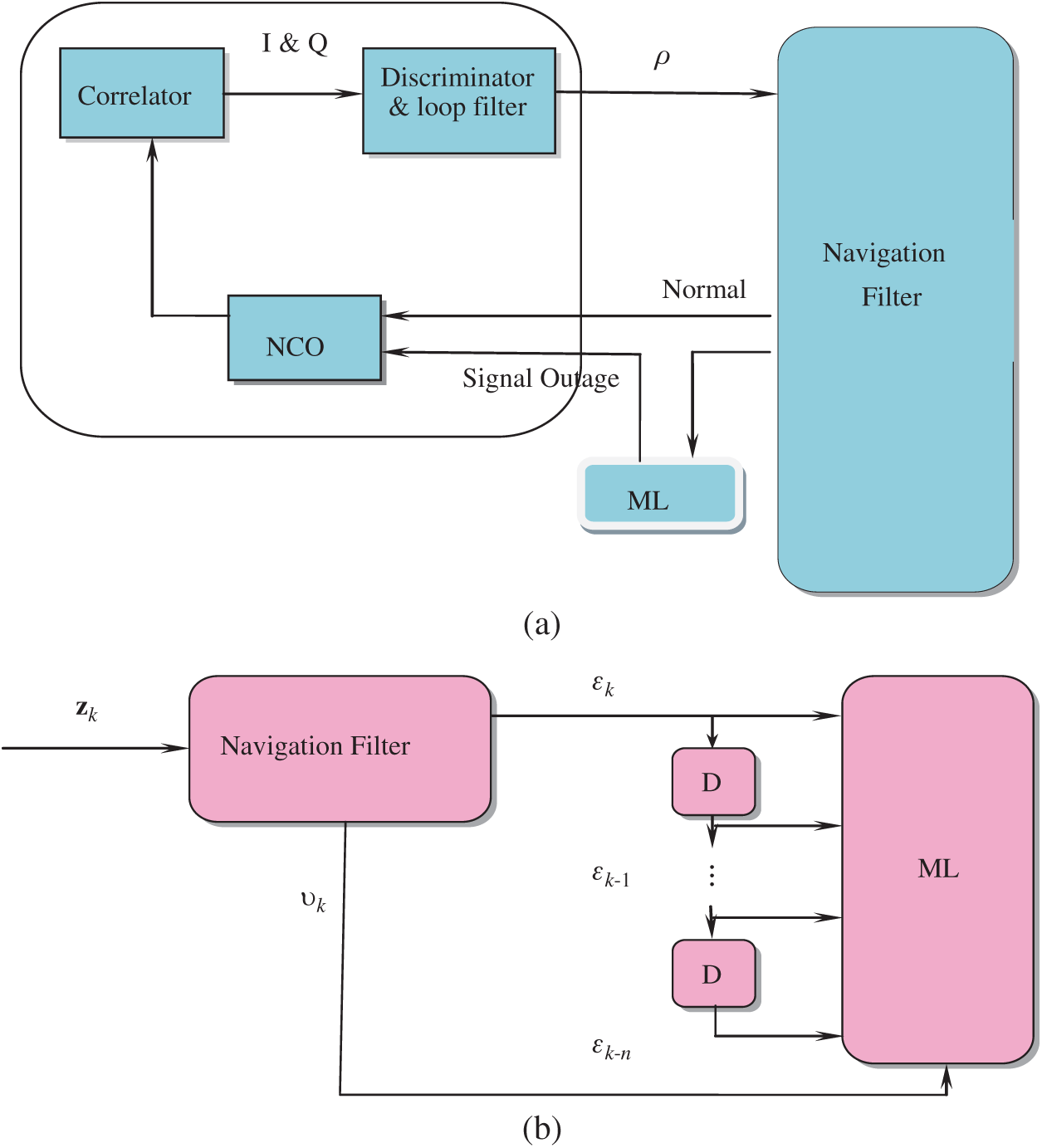
Figure 5: (a) The vector tracking loop assisted by the machine learning (ML) module; and (b) the training procedure for the ML

5  Illustrative Examples

Simulation experiments had been carried out to evaluate the navigation performance for the proposed approach, i.e., with ML aiding for overcoming the problem of signal outage, in comparison with the standard VTL designs. The computer codes were developed by the authors using the Matlab® software. The commercial software Satellite Navigation (SatNav) toolbox for Matlab® by GPSsoft LLC. Reference [27] was employed for generating the satellite positions and pseudoranges. A simulated vehicle trajectory originating from the position of North 25.1492 degrees and East 121.7775 degrees at an altitude of 100 m. This is equivalent to [−3042329.2\enskip4911080.2\enskip2694074.3]T m in the WGS-84 ECEF coordinate system. The location of the origin is defined as the (0, 0, 0) m location in the local tangent East-North-Up (ENU) frame.

The test trajectory is shown in Fig. 6. Shown in Fig. 7, the satellite constellation at the initial time of simulation involves 9 SV’s available in the open sky, where the satellites are numbered with a space vehicle identifier (SV ID). The skyplots for the three scenarios are indicated by three blocks. In Scenario 1, the GPS signals are available on the west where there are 4 satellites available. In this scenario, signal outage at two time intervals has been assumed, including 125–165 s and 245–285 s, respectively. In Scenario 2, the GPS signals are available on the south where there are 4 satellites available on the south, while in Scenario 3, one satellite signal (i.e., SV 6) was blocked out and the case where only 3 GPS signals available are involved. The measurement noise variances rρi are assumed a priori known, which is set as 9 m2. Let each of the white-noise spectral amplitudes that drive the random walk position states be Sp=1.0 (m/sec2)/rad/sec. In addition, let the clock model spectral amplitudes be Sf=0.4 (10−18)sec and Sg=1.58 (10−18)sec−1. These spectral amplitudes were used to find the Qk parameters in Eq. (20).

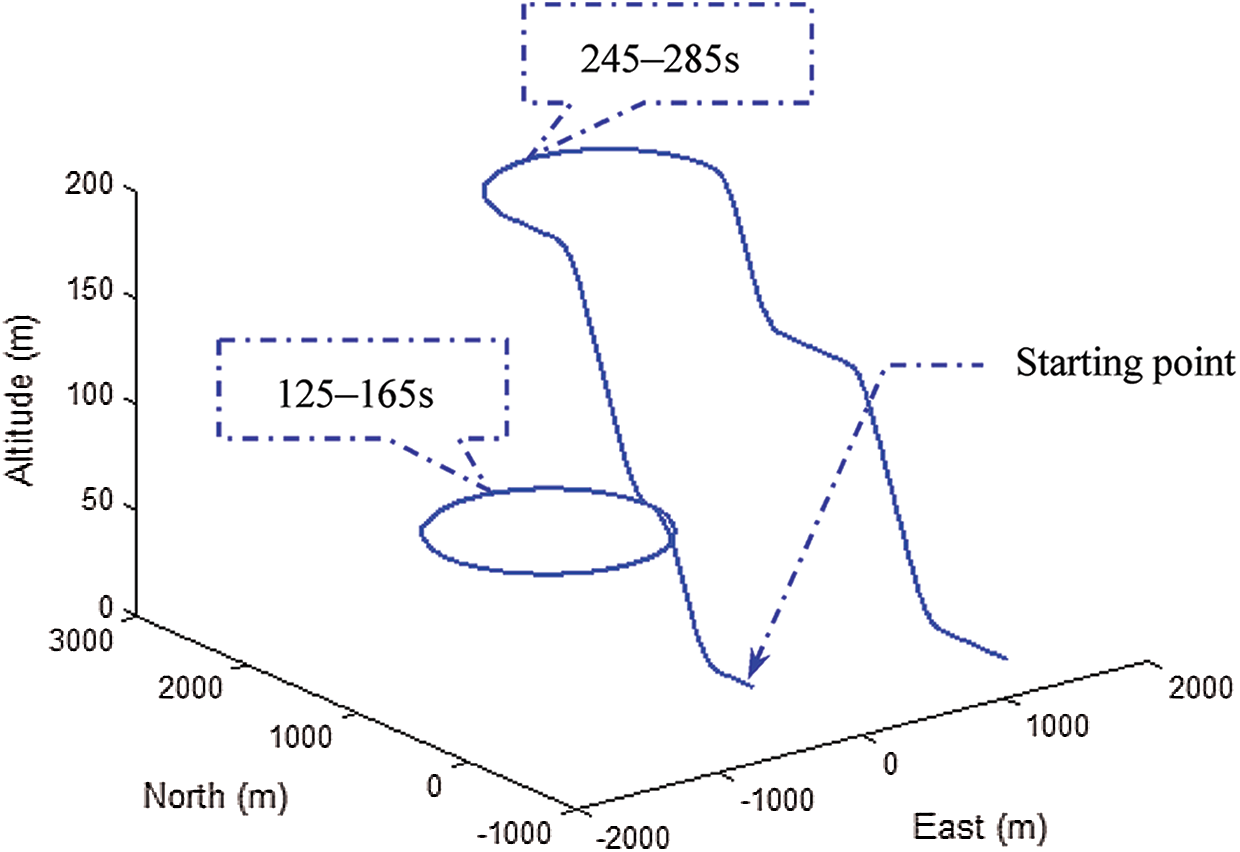
Figure 6: The vehicle trajectory for simulation

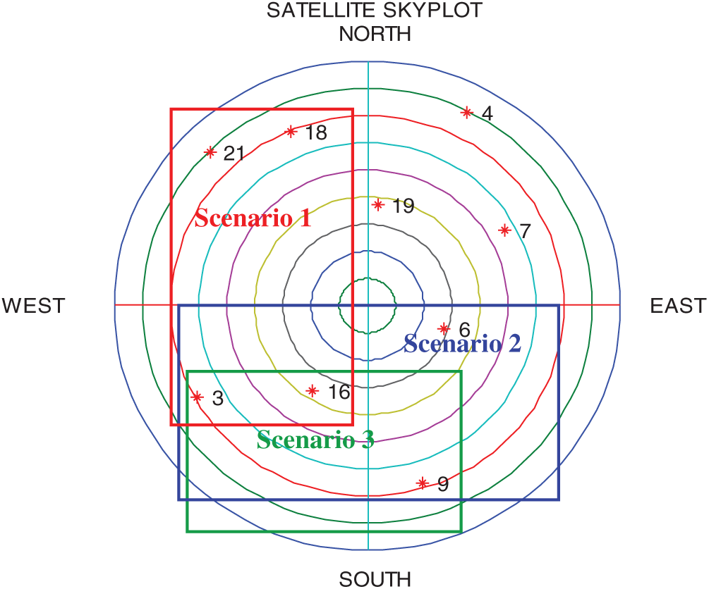
Figure 7: The satellite constellation at the initial time of simulation indicates that there are 9 SV’s available in the open sky; the visible satellites for the three scenarios involved are indicated by three blocks

The results for the three scenarios are discussed as follows.

(1) Scenario 1: 4 GPS signals available on the west

In this case, there are 4 GPS signals available with the visible satellites inside the red block in Fig. 7. The cases that GPS signal outages occur on the east at the time interval 125–165 s and 245–285 s, respectively, are simulated. The results demonstrate the effectiveness for the performance enhancement. Fig. 8 provides the position errors for the standard VTL as compared to that assisted by the SVM at the time interval 125–165 s. In the case that GPS signal outage on the east at the time interval 245–285 s is simulated, the results are shown in Fig. 9. The results based on the VTL with the various ML algorithms, including RBFNN, ANFIS, and SVM are compared. Fig. 10 provides comparison of position RMS errors for the three approaches and the SVM outperforms the other two.

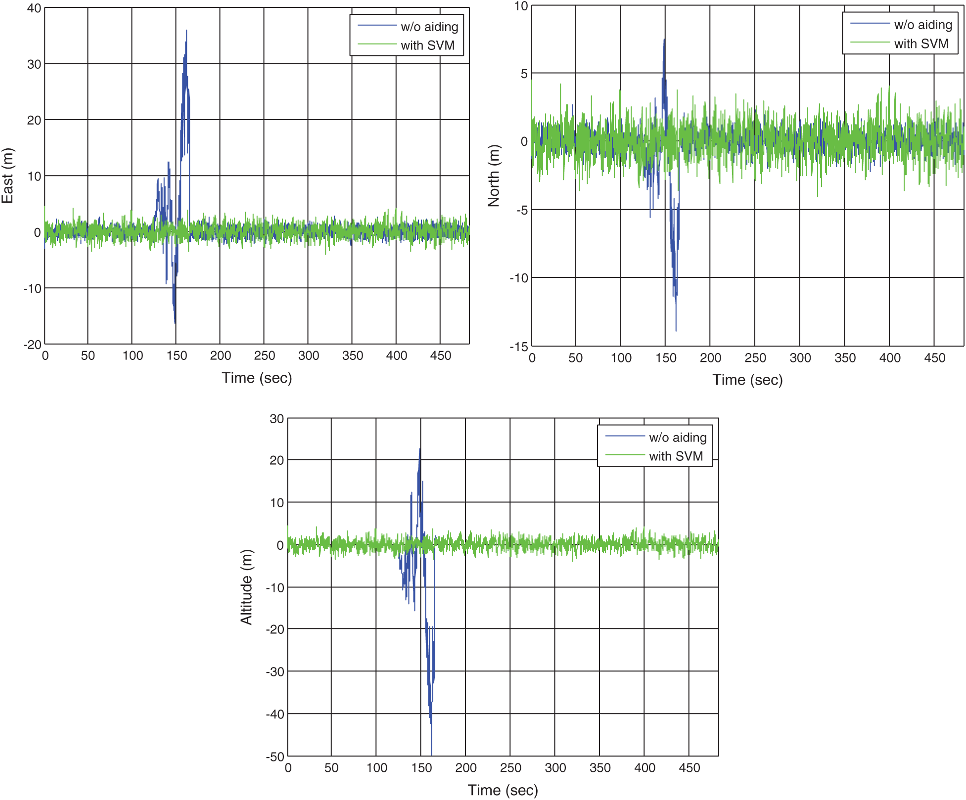
Figure 8: Position errors for the VTL without and with the SVM: Scenario 1 with signal outage at time interval 125–165 s

Figure 9: Position errors for the VTL without and with the SVM: Scenario 1 with signal outage at time interval 245–285 s

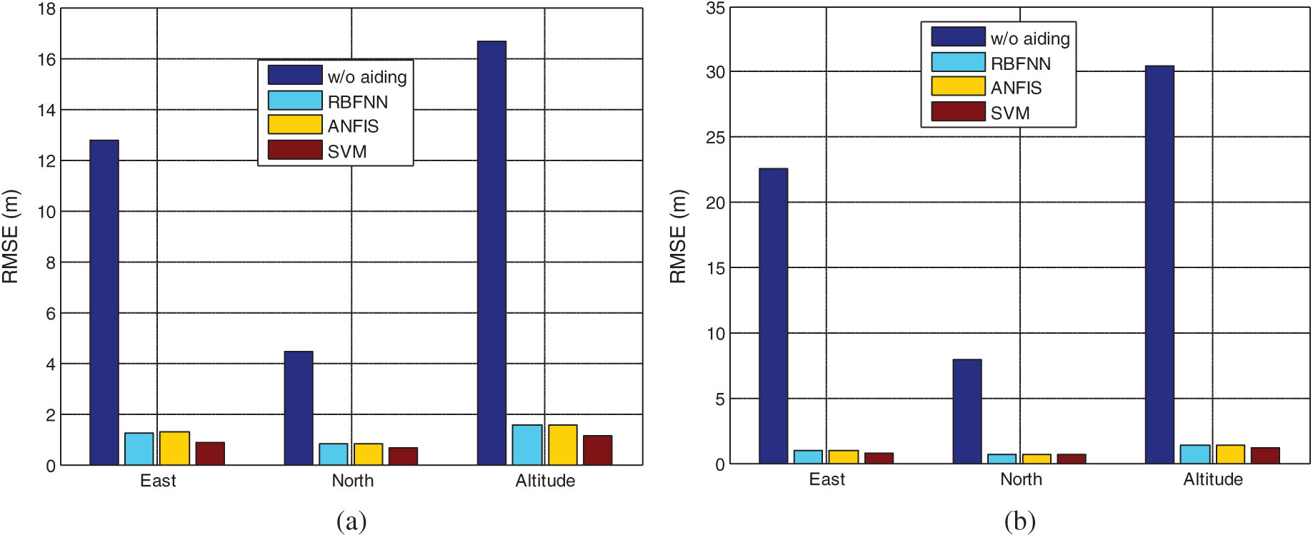
Figure 10: Comparison of position RMS errors based on the three ML approaches for Scenario 1 with signal outage at time intervals: (a) 125–165 s; (b) 245–285 s

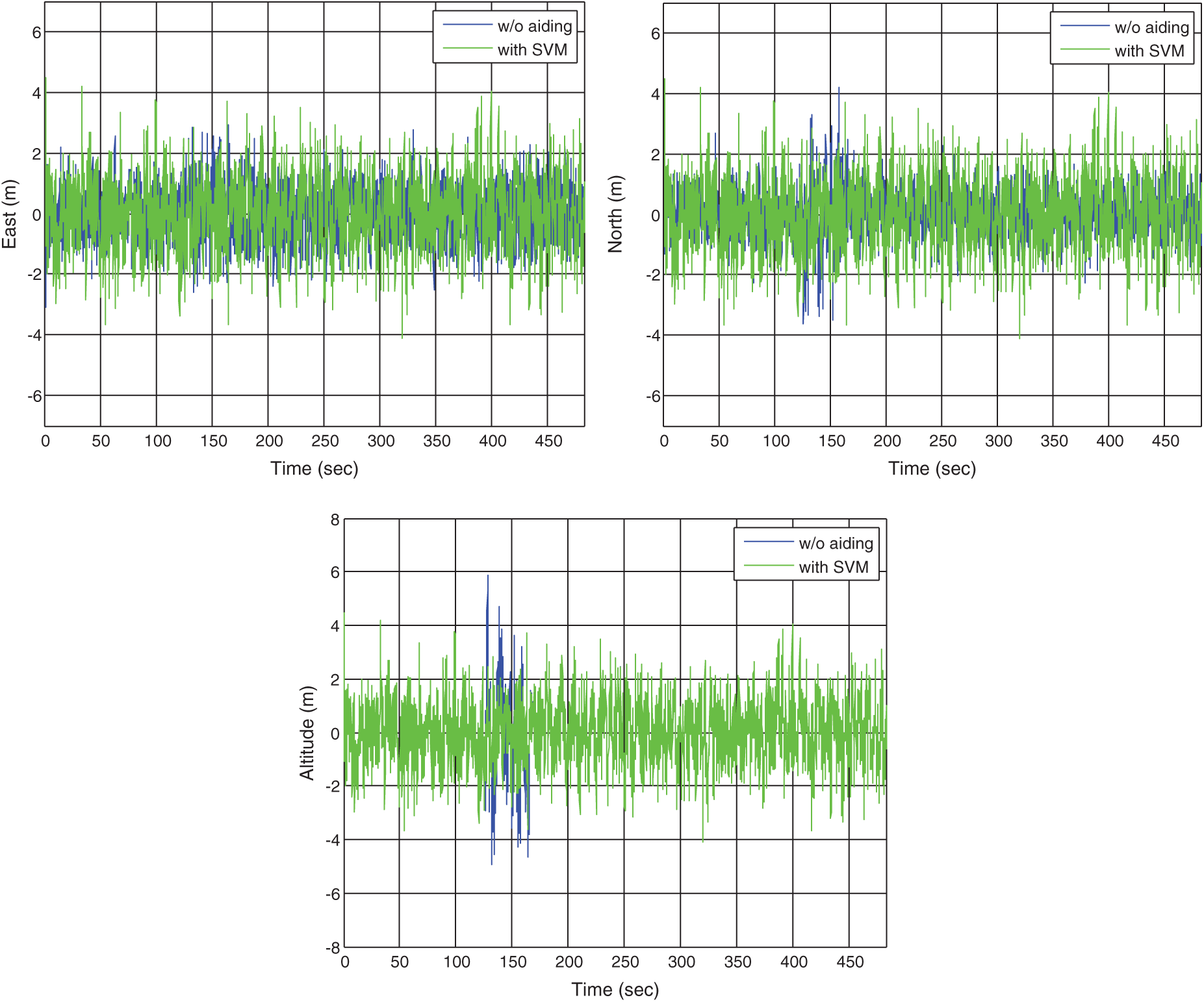
Figure 11: Position errors for the VTL without and with the SVM for Scenario 2

(2) Scenario 2: 4 GPS signals available on the south

In the second example, it is assumed that there are 4 GPS signals available on the south with visible satellites inside the blue block in Fig. 7. The GPS signal outage on the north is simulated. Fig. 11 provides the position errors for the standard VTL as compared to that assisted by SVM. Comparison of position RMS errors for the three ML approaches: RBFNN, ANFIS, and SVM, is shown in Fig. 12.

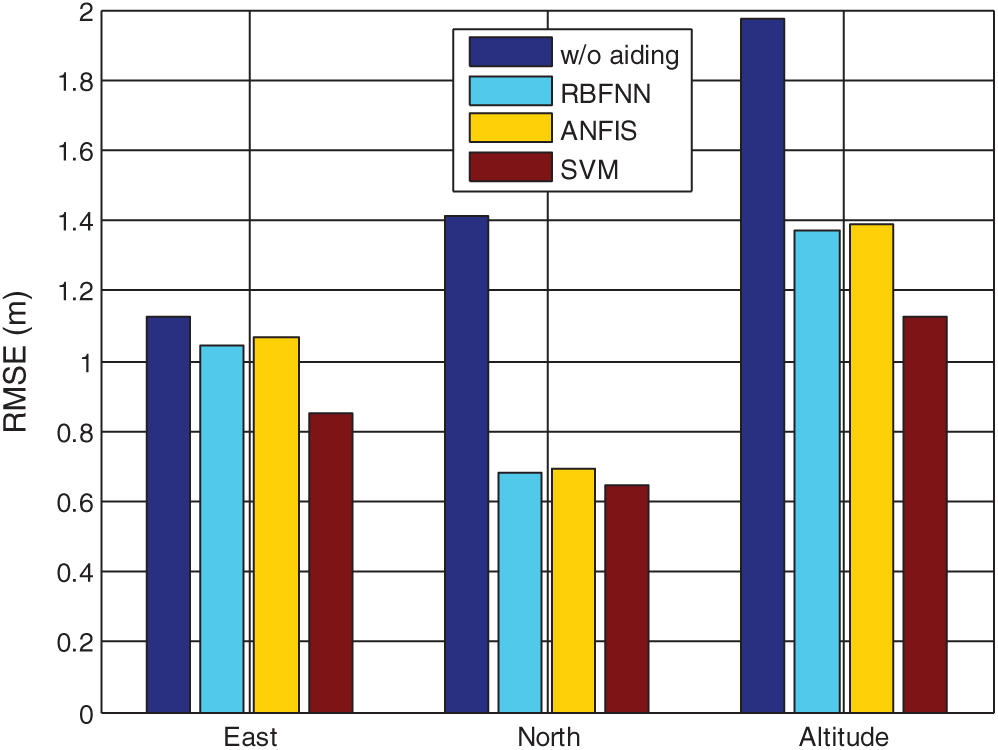
Figure 12: Comparison of position RMS errors for the three approaches for Scenario 2

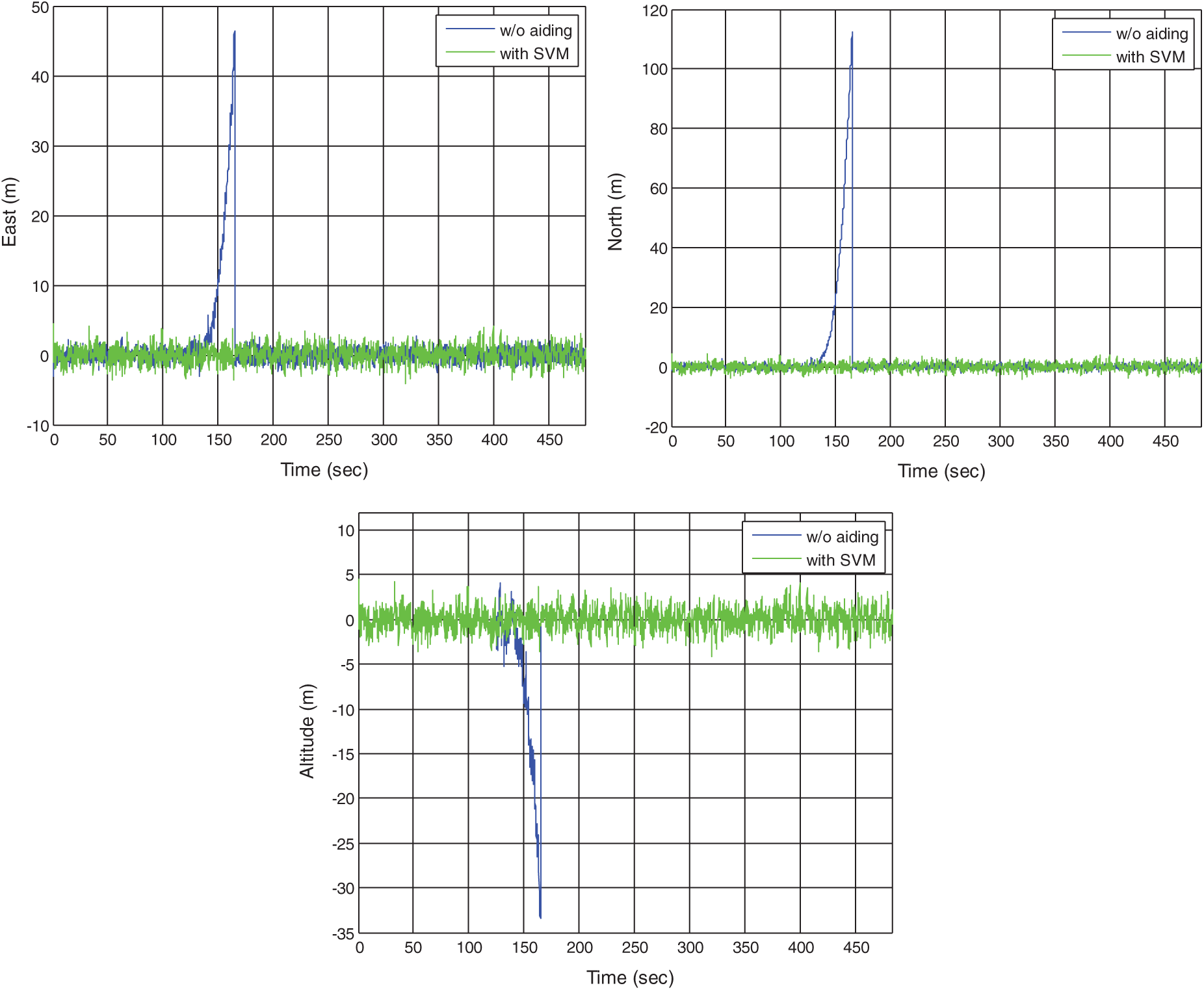
Figure 13: Position errors for the VTL without and with the SVM (3 GPS signals available)

(3) Scenario 3: 3 GPS signals available on the south

In the third example, a case that only 3 GPS signals are available is simulated. The visible satellites for this example are indicated inside the green block in Fig. 7. Fig. 13 provides the position errors for the standard VTL as compared to that assisted by SVM. The results based on the VTL with the three ML approaches are shown as in Fig. 14. The example has demonstrated remarkable performance improvement in such a case of relatively poor geometry. Comparison of position RMS errors for the various approaches is shown as in Fig. 15 which shows the SVM method is very promising.

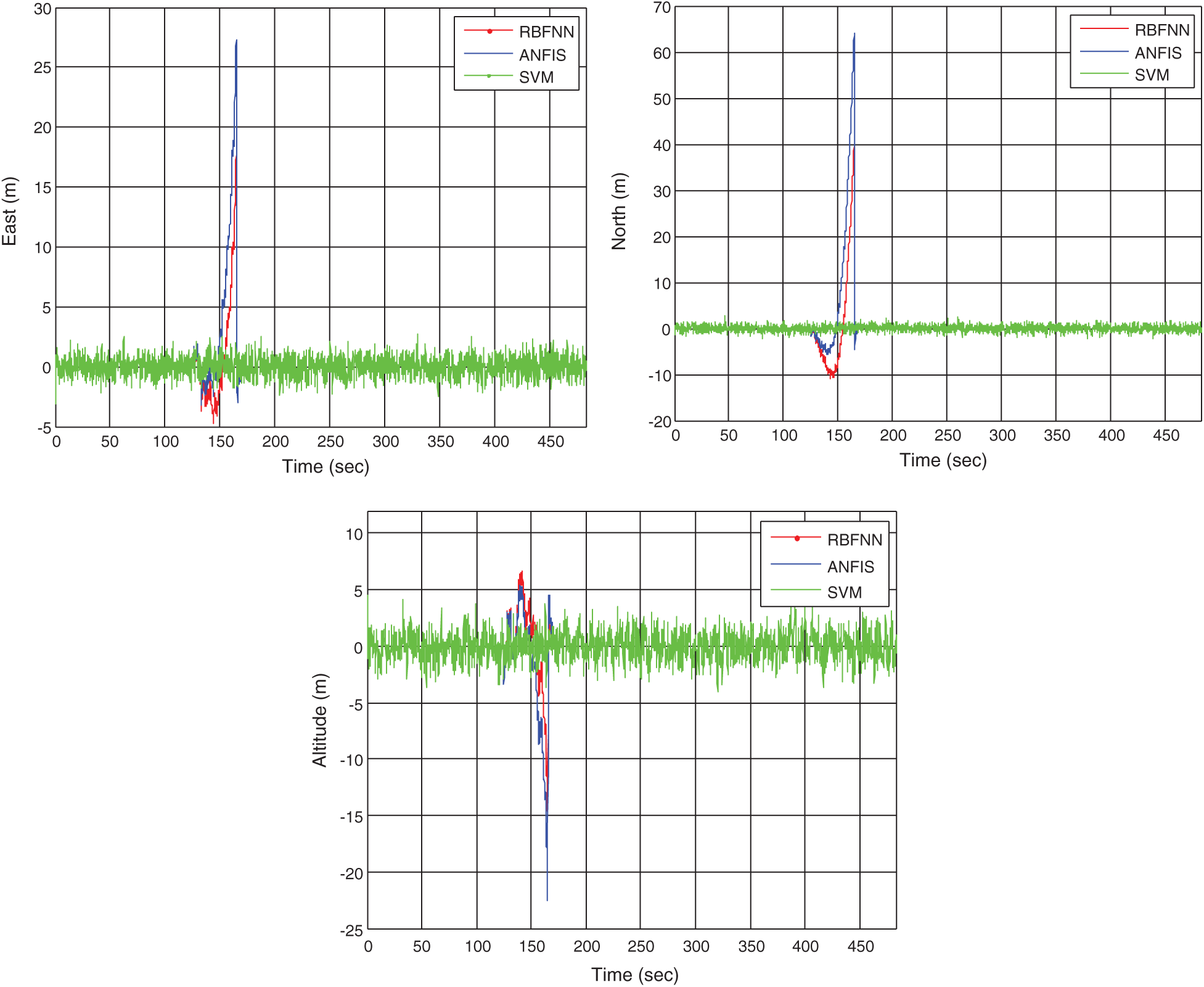
Figure 14: Position errors for the VTL with the RBFNN, ANFIS, and SVM (3 GPS signals available)

In addition to positioning accuracy, the computational cost/convergent time is also studied. In the time intervals of GPS signal outages, which are set to be 40 s in the simulation. The total times for executing the navigation Kalman filter with ML module is about 18–19 s for RBFNN, 5-6 s for ANFIS, and 2–3 s for SVM, respectively. The SVM possesses better computational efficiency.

Figure 15: Comparison of position RMS errors for the three approaches (3 GPS signals available)

6  Conclusions

This paper investigates the incorporation of the SVM algorithm into the vector tracking loop for improving performance in limited visibility of GPS satellites. The method makes use of the SVM module to predict the code phase from the Kalman filter, and to bridge the GPS signal so as to prevent the error growth during signal outage. In addition to the SVM, two other types of ML algorithms involved are the RBFNN and the ANFIS. Several examples have been provided for illustration.

The ML assisted architecture exhibit remarkable benefit in the case where sufficient numbers of visible satellites are available. Some performance comparison for the three types of algorithms has been also provided. Based on the reports from the literatures for various applications, different results are revealed regarding the performance comparison for various ML algorithms according to different situations. In this preliminary study, we have concentrate on the feasibility of performance improvement based on the support of ML modules. The results show that the VTL based on the proposed design has demonstrated the capability of ensuring proper functioning of navigation system and provide improved performance, especially for the GPS signal outage environment.The SVM in the case of 3 GPS signals available has demonstrated very promising results, in terms of both accuracy and computational efficiency. Further work on the test and evaluation of the design can be carried out such that more advanced design for better applicability can be obtained based on the idea addressed in the paper.

Funding Statement: This work has been partially supported by the Ministry of Science and Technology, Taiwan (Grant numbers MOST 104-2221-E-019-026-MY3 and MOST 109-2221-E-019-010).

Conflicts of Interest: The authors declare that they have no conflicts of interest to report regarding the present study.

References

 1.  K. Borre, D. M. Akos, N. Bertelsen, P. Rinder and S. H. Jensen, A Software-Defined GPS and Galileo Receiver. Boston, MA, USA: Birkhäuser, 2007. [Google Scholar]

 2.  B. Y. J. Tsui, Fundamentals of Global Positioning System Receivers: A Software Approach, 2nd ed., New York, NY, USA: John Wiley & Sons, 2005. [Google Scholar]

 3.  T. Pany and B. Eissfeller, “Use of a vector delay lock loop receiver for GNSS signal power analysis in bad signal conditions,” in Proc. 2006 IEEE/ION Position, Location, and Navigation Symp., Coronado, CA, USA, pp. 893–903, 2006. [Google Scholar]

 4.  M. Lashley, D. M. Bevly and J. Y. Hung, “Performance analysis of vector tracking algorithms for weak GPS signals in high dynamics,” IEEE Journal of Selected Topics in Signal Processing, vol. 3, no. 4, pp. 661–673, 2009. [Google Scholar]

 5.  M. Lashley and D. M. Bevly, “Comparison in the performance of the vector delay/frequency lock loop and equivalent scalar tracking loops in dense foliage and urban canyon,” in Proc. 24th Int. Technical Meeting of the Institute of Navigation, Portland, OR, USA, pp. 1786–1803, 2011. [Google Scholar]

 6.  Z. Zhu, Z. Cheng, G. Tang, S. Li and F. Huang, “EKF based vector delay lock loop algorithm for GPS signal tracking,” in Proc. 2010 Int. Conf. on Computer Design and Applications, Qinhuangdao, China, vol. 4, pp. 352–356, 2010. [Google Scholar]

 7.  S. Peng, Y. Morton and R. Di, “A multiple-frequency GPS software receiver design based on a vector tracking loop,” in Proc. 2012 IEEE/ION Position, Location and Navigation Symp., Myrtle Beach, SC, USA, pp. 495–505, 2012. [Google Scholar]

 8.  H. Li and J. Yang, “Analysis and simulation of vector tracking algorithms for weak GPS signal,” in Proc. 2nd Int. Asia Conf. on Informatics in Control, Automation and Robotics, Wuhan, China, pp. 215–218, 2010. [Google Scholar]

 9.  N. Kanwal, “Vector tracking loop design for degraded signal environment,” Master thesis. Tampere University of Technology, Finland, 2010. [Google Scholar]

10. K. H. Kim, G. I. Jee and S. H. Im, “Adaptive vector-tracking loop for low-quality GPS signals,” International Journal of Control, Automation, and Systems, vol. 9, no. 4, pp. 709–715, 2011. [Google Scholar]

11. D.-J. Jwo, Z.-M. Wen and Y.-C. Lee, “Vector tracking loop assisted by the neural network for GPS signal blockage,” Applied Mathematical Modelling, vol. 39, no. 19, pp. 5949–5968, 2015. [Google Scholar]

12. S. C. Stubberud, R. N. Lobbia and M. Owen, “An adaptive extended Kalman filter using artificial neural networks,” in Proc. IEEE the 34th Conf. on Decision & Control, New Orleans, LA, USA, pp. 1852–1856, 1995. [Google Scholar]

13. A. Asadian, B. Moshiri and J. Rezaie, “Robustness assessment of intelligent information fusion techniques in navigation systems encountering satellite outage,” in Proc. 4th Int. Conf. on Innovations in Information Technology, Dubai, United Arab Emirates, pp. 46–50, 2007. [Google Scholar]

14. M. Aslinezhad, A. Malekijavan and P. Abbasi, “ANN-assisted robust GPS/INS information fusion to bridge GPS outage,” EURASIP Journal on Wireless Communications and Networking, vol. 129, pp. 1–18, 2020. [Google Scholar]

15. I. Yilmaz and O. Kaynar, “Multiple regression, ANN (RBF, MLP) and ANFIS models for prediction of swell potential of clayey soils,” Expert Systems with Applications, vol. 38, no. 5, pp. 5958–5966, 2011. [Google Scholar]

16. E. Khadangi, H. R. Madvar and M. M. Ebadzadeh, “Comparison of ANFIS and RBF Models in Daily Stream Flow Forecasting,” in Proc. 2nd Int. Conf. on Computer, Control and Communication, Karachi, Pakistan, pp. 1–6, 2009. [Google Scholar]

17. J.-S. R. Jang, “ANFIS: Adaptive-network-based fuzzy inference system,” IEEE Transactions on Systems, Man, and Cybernetics, vol. 23, no. 3, pp. 665–685, 1993. [Google Scholar]

18. A. Zamani, M. R. Sorbi and A. A. Safavi, “Application of neural network and ANFIS model for earthquake occurrence in Iran,” Earth Science Informatics, vol. 6, no. 2, pp. 71–85, 2013. [Google Scholar]

19. N. Pramanik and R. K. Panda, “Application of neural network and adaptive neurofuzzy inference systems for river flow prediction,” Hydrological Sciences Journal, vol. 54, no. 2, pp. 247–260, 2009. [Google Scholar]

20. K. Ahmadaali, A. Liaghat, N. Heydari and O. B. Haddad, “Application of artificial neural network and adaptive neural-based fuzzy inference system techniques in estimating of virtual water,” International Journal of Computer Applications, vol. 76, no. 6, pp. 12–19, 2013. [Google Scholar]

21. J. Sadoon and B. B. Üstündağ, “Fused and modified evolutionary optimization of multiple intelligent systems using ANN, SVM approaches,” Computers, Materials & Continua, vol. 66, no. 2, pp. 1479–1496, 2021. [Google Scholar]

22. B. E. Boser, I. M. Guyon and V. N. Vapnik, “A training algorithm for optimal margin classifier,” in Proc. 5th ACM Workshop on Computational Learning Theory, Pittsburgh, PA, USA, pp. 144–152, 1992. [Google Scholar]

23. C. Cortes and V. Vapnik, “Support-vector networks,” Machine Language, vol. 20, no. 3, pp. 273–297, 1995. [Google Scholar]

24. M. O. Efe, “A Comparison of ANFIS, MLP and SVM in identification of chemical processes,” in Proc.2009 IEEE Int. Symp. on Intelligent Control, Saint Petersburg, Russia, pp. 689–694, 2009. [Google Scholar]

25. M. Buyukyildiz and S. Y. Kumcu, “An estimation of the suspended sediment load using adaptive network based fuzzy inference system, support vector machine and artificial neural network models,” Water Resources Management, vol. 31, no. 4, pp. 1343–1359, 2017. [Google Scholar]

26. R. G. Brown and P. Y. C. Hwang, Introduction to Random Signals and Applied Kalman Filtering. New York, NY, USA: John Wiley & Sons, 1997. [Google Scholar]

27. GPSoft LLC., Satellite Navigation Toolbox 3.0 User’s Guide. Athens, OH, USA, 2003. [Google Scholar]

This work is licensed under a Creative Commons Attribution 4.0 International License, which permits unrestricted use, distribution, and reproduction in any medium, provided the original work is properly cited.