DOI:10.32604/cmc.2021.017914
| Computers, Materials & Continua DOI:10.32604/cmc.2021.017914 | |
| Article |
Deep Learning and Entity Embedding-Based Intrusion Detection Model for Wireless Sensor Networks
Department of Computer Science, College of Computer Engineering and Sciences, Prince Sattam bin Abdulaziz University, Al-Kharj, 11942, Saudi Arabia
*Corresponding Author: Bandar Almaslukh. Email: b.almaslukh@psau.edu.sa
Received: 17 February 2021; Accepted: 11 April 2021
Abstract: Wireless sensor networks (WSNs) are considered promising for applications such as military surveillance and healthcare. The security of these networks must be ensured in order to have reliable applications. Securing such networks requires more attention, as they typically implement no dedicated security appliance. In addition, the sensors have limited computing resources and power and storage, which makes WSNs vulnerable to various attacks, especially denial of service (DoS). The main types of DoS attacks against WSNs are blackhole, grayhole, flooding, and scheduling. There are two primary techniques to build an intrusion detection system (IDS): signature-based and data-driven-based. This study uses the data-driven approach since the signature-based method fails to detect a zero-day attack. Several publications have proposed data-driven approaches to protect WSNs against such attacks. These approaches are based on either the traditional machine learning (ML) method or a deep learning model. The fundamental limitations of these methods include the use of raw features to build an intrusion detection model, which can result in low detection accuracy. This study implements entity embedding to transform the raw features to a more robust representation that can enable more precise detection and demonstrates how the proposed method can outperform state-of-the-art solutions in terms of recognition accuracy.
Keywords: Wireless sensor networks; intrusion detection; deep learning; entity embedding; artificial neural networks
With the variety of applications of wireless sensor networks (WSNs) in areas such as environmental observation, smart cities, military surveillance, and healthcare [1], there have been an increasing number of security breaches in such networks. A primary factor is limited computing resources such as processing, storage, memory, and power, enabling such denial of service (DoS) attacks as blackhole, scheduling, grayhole, and flooding. DoS attack detection is considered a machine learning task, i.e., a supervised classification problem. Such methods include traditional machine learning and deep learning.
Deep learning often outperforms traditional machine learning on unstructured data problems such as image and audio recognition and natural language processing, and is increasingly regarded as the ideal solution for such data. This has led to the question of whether these methods can be similarly successful with structured (tabular) data, such as is used in this study. Structured data are organized in a tabular format whose columns and rows represent features and data points, respectively. Current state-of-the-art solutions for structured data are ensemble methods such as random forest [2] and gradient boosted tree [3], and deep learning with entity embedding [4] has performed at least as well on tabular data.
The present study proposes an end-to-end ANN architecture with entity embedding that outperforms recent state-of-the-art intrusion detection models for WSNs on a public WSN-DS dataset [5]. The proposed model does not depend on a complex ensemble model and handcrafted feature engineering. It considers features as categorical variables and maps them into m-dimensional vectors of continuous variables that transform a raw feature in a more robust representation. The mapping is automatically learned through supervised learning of standard neural networks.
The remainder of this paper is organized as follows. Section 2 examines related studies. Section 3 explains materials and methods used in the proposed solution. Section 4 discusses experiments using the proposed model on the WSN-DS dataset. Section 5 presents conclusions and suggested future research.
Applications of WSNs include recognizing climate changes, monitoring habitats and environments, and other surveillance applications [6]. Several security-based methods for WSNs have been proposed, including key exchange protocol, authentication, secure routing protocol, and security solutions targeting a specific type of attack [7,8]. The intrusion detection system (IDS) is a promising solution to identify and defend against WSN attacks [9]. When detecting an attack, the IDS raises an alarm to notify the controller to take action [9,10]. However, WSNs are exposed to numerous security threats, such as DoS, which can degrade their performance. DoS attacks can target the protocol stack, or different layers of sensors [11–13]. To detect attacks, network traffic is examined, and an appropriate security mechanism is used [14].
IDSs use two main approaches. Rule- or signature-based IDS [15] can accurately detect well-known attacks, but not a zero-day attack whose signatures do not exist in intrusion signature data. Anomaly-based (data-driven) IDSs detect intrusions by matching abnormal resource utilization and/or traffic patterns against normal behavior. Although anomaly-based IDSs can detect both well-known and zero-day attacks, they have more false positives and false negatives [15]. The present study lists related work using anomaly-based IDSs for WSNs, as they are more closely related to the proposed method. Current IDS methods for WSNs include genetic algorithms and fuzzy rule-based modeling [16], support vector machine (SVM) [17], artificial neural networks [18], Bayesian networks and random tree [19], and random forest [20]. Their limitations were evaluated on the KDD dataset [21] that was collected for computer networks such as local area networks (LANs) and wide area networks (WANs), but not for WSNs with special characteristics. Some work has used self-made WSN datasets [22–24] that are not publicly available. We used the publicly available WSN-DS dataset [5].
Some work has been evaluated on the WSN-DS dataset [5], which was collected specifically for WSNs. An artificial neural network was used [5] to build the classifier; feature selection using the information gain ratio and a bagging algorithm was proposed [25]; and naive Bayes, SVM, decision tree, k-nearest neighbor (KNN), and a convolutional neural network (CNN) were utilized [26]. The limitation of these methods is that they use raw features directly. This can be addressed by transforming raw features to a more robust representation using entity embedding.
We used entity embedding to develop a more accurate classification, and experimentally demonstrated how the proposed method can outperform state-of-the-art solutions.
This section has six subsections. Subsection 3.1 describes the dataset. Subsection 3.2 explains the artificial neural network (ANN) model primarily used in this work. Subsection 3.3 examines the entity embedding of categorical variables [4], the essential technique used in this study. Subsection 3.4 illustrates the proposed architecture. Subsection 3.5 explains the evaluation of the model. Subsection 3.6 presents hyperparameter selection strategies.
We used the WSN-DS simulated dataset [5] to build and evaluate the proposed model. The dataset was created to recognize several types of DoS attacks as well as normal traffic. It contains four DoS attack types: blackhole, grayhole, flooding, and scheduling, with 17 features, describing the state of each sensor in WSN, extracted from the Low Energy Aware Cluster Hierarchy (LEACH) routing protocol. These and the target variables (label) are shown in Tab. 1. Fig. 1 shows the data distribution over normal and different types of attacks from the WSN-DS dataset. It should be noted that such extreme imbalances in the class distribution require a specific type of metric to evaluate model performance, as the accuracy is dominated by the majority class (normal).
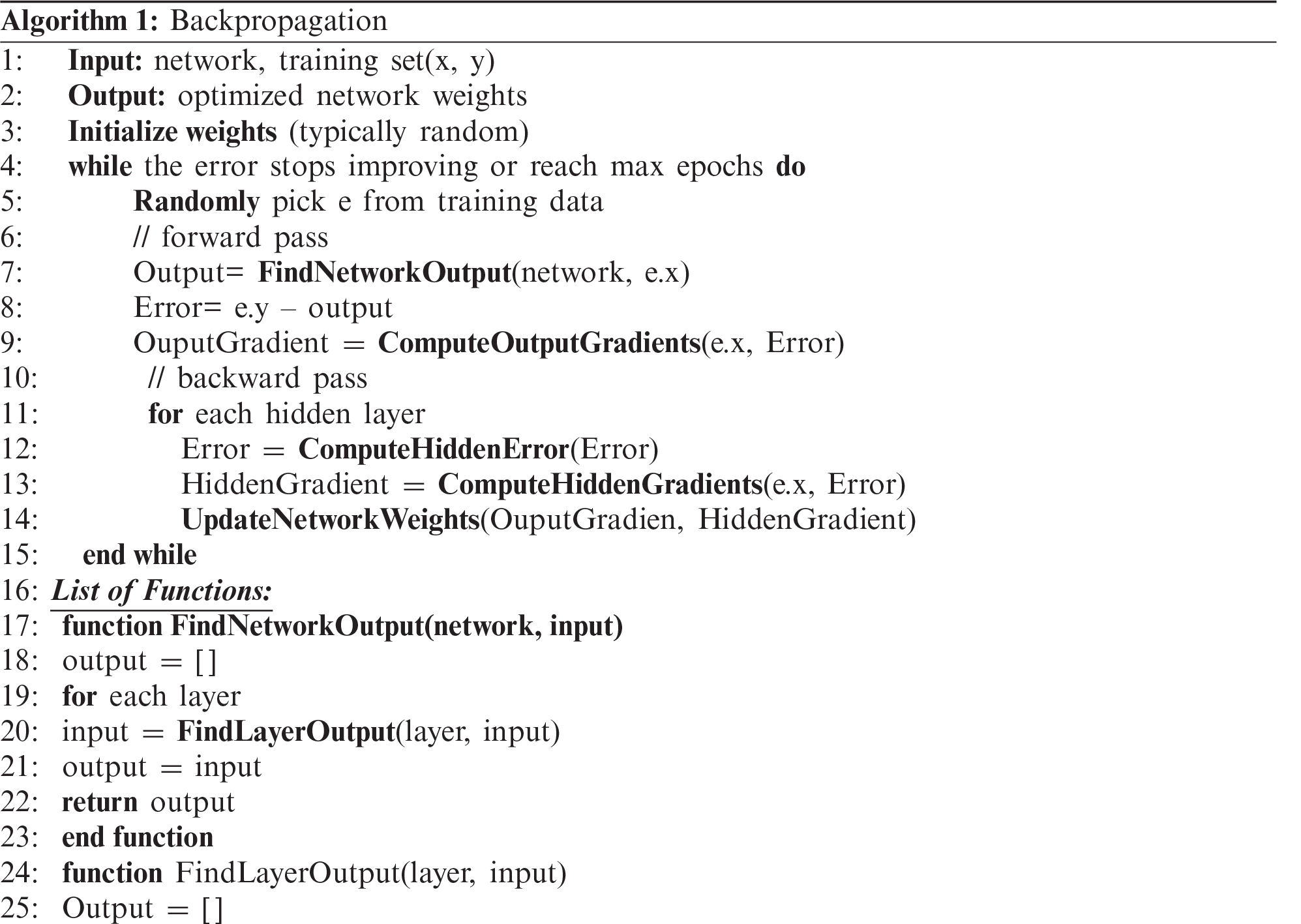
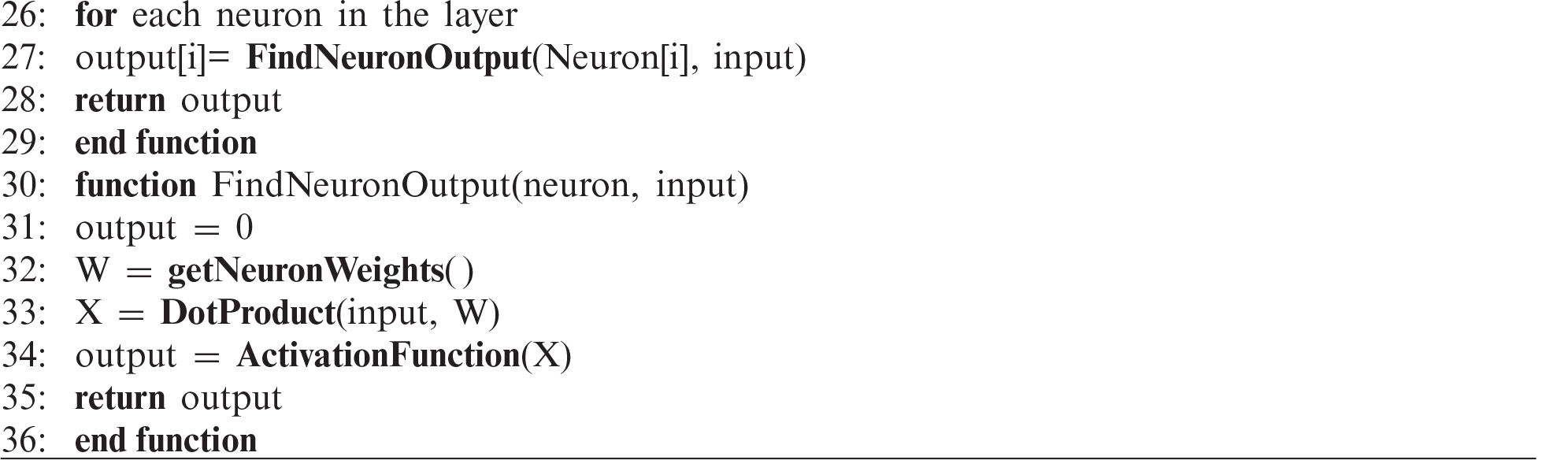
We explore the ANN, the main model used in this paper. The multilayer perceptron (MLP) is the primary ANN architecture [27]. As shown in Fig. 2, MLP has three types of layers: one-input layer, one/more-hidden layer, and one output layer. As these layers are densely connected, many weights (parameters) must be configured. These are fine-tuned during the backpropagation algorithm [28], as shown in Algorithm 1. The input of the algorithm is a set of input-output
The goal of backpropagation is to fine-tune a network’s weights through a sequence of forward and backward iterations to minimize the cost function until the error stops improving or the maximum number of epochs is reached. The algorithm first initializes the weights of the network using a statistical initializer.
Table 1: List of features with abbreviation, description, and number of levels
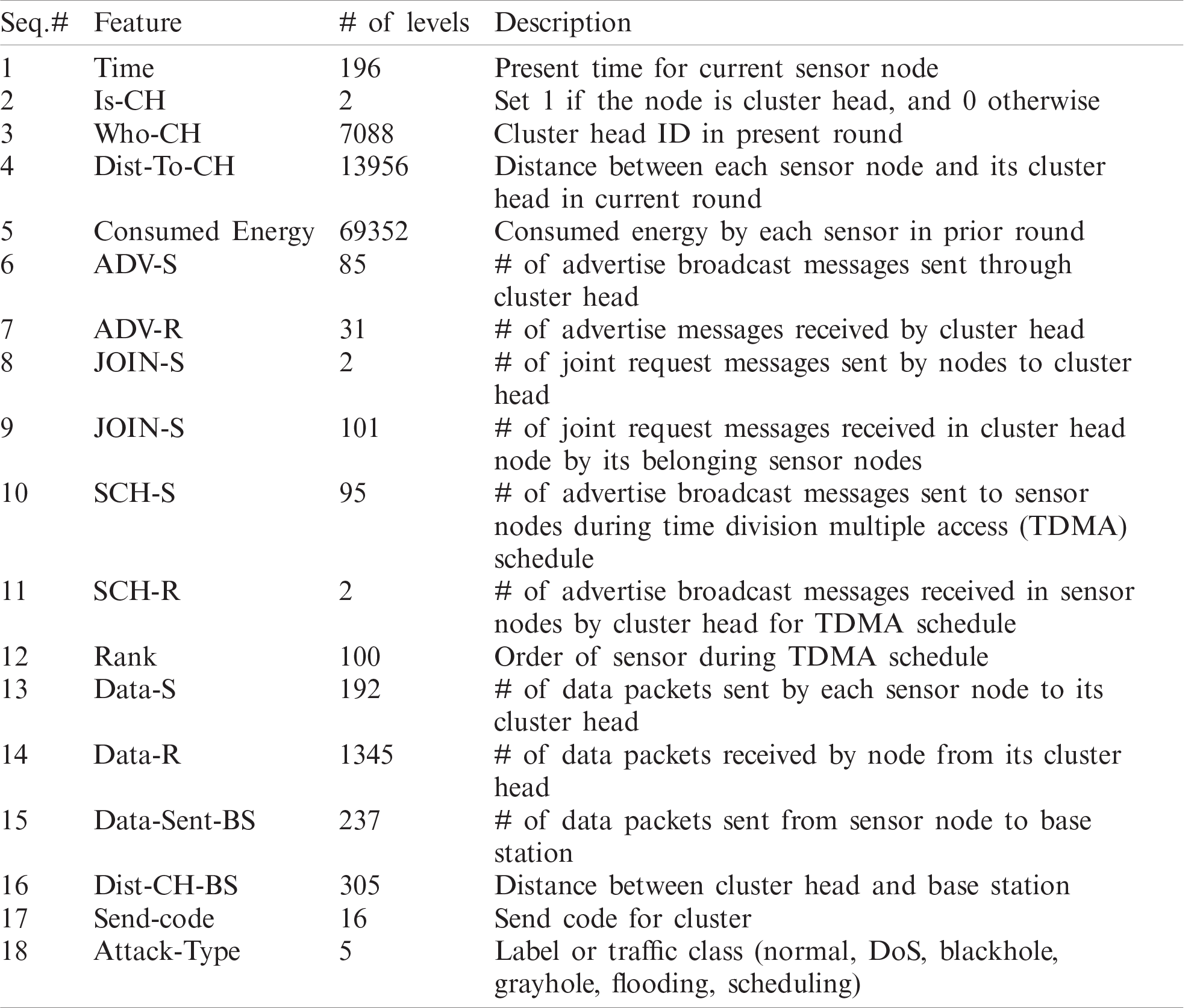
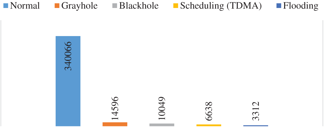
Figure 1: Data distribution over normal and different types of attacks deduced from WSN-DS dataset
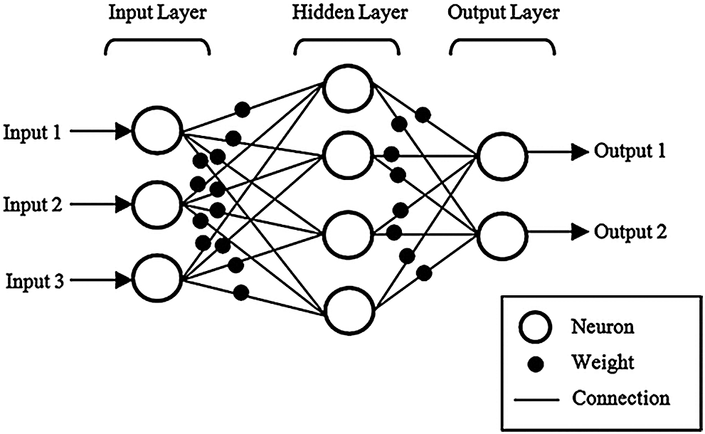
Figure 2: Basic ANN architecture [29]
A forward step finds the network output for randomly selected training examples
where
After applying the forward step, we get
Then the gradient of error is calculated by computing the partial derivative of error with respect to each weight.
The second step is backward, and calculation is performed from the output layer toward the first hidden layer. The gradient and error are computed using the chain rule [28] for each hidden layer. All network weights are updated according to the gradient of the output and all hidden layers.
3.3 Entity Embedding of Categorical Variables
Entity embedding of categorical variables [4] is the primary technique used in this paper, which maps them into m-dimensional vectors of continuous variables. Supervised learning of a standard neural network is used to learn the mapping, as explained previously.
As an example, assume that entity embedding is applied over a day of the week as a categorical variable of the neural network model. This leads to the development of a
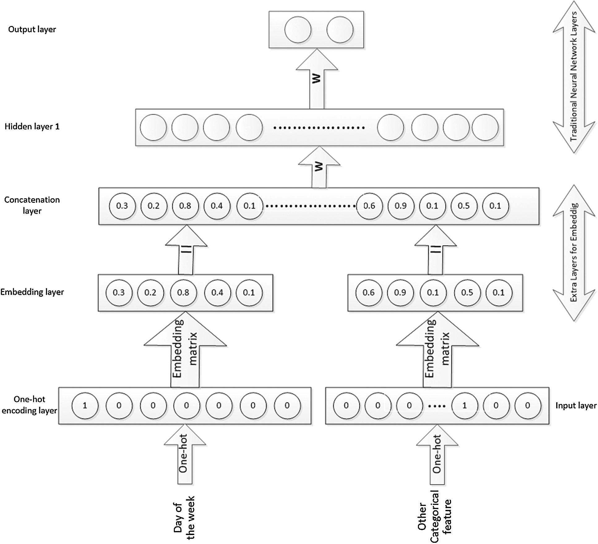
Figure 3: Proposed model architecture
For the above example, the one-hot encoding input layer includes seven neurons that indicate the number of levels of the categorical variable, and the embedding layer has four neurons, corresponding to the desired mapping dimension, as shown in Fig. 3.
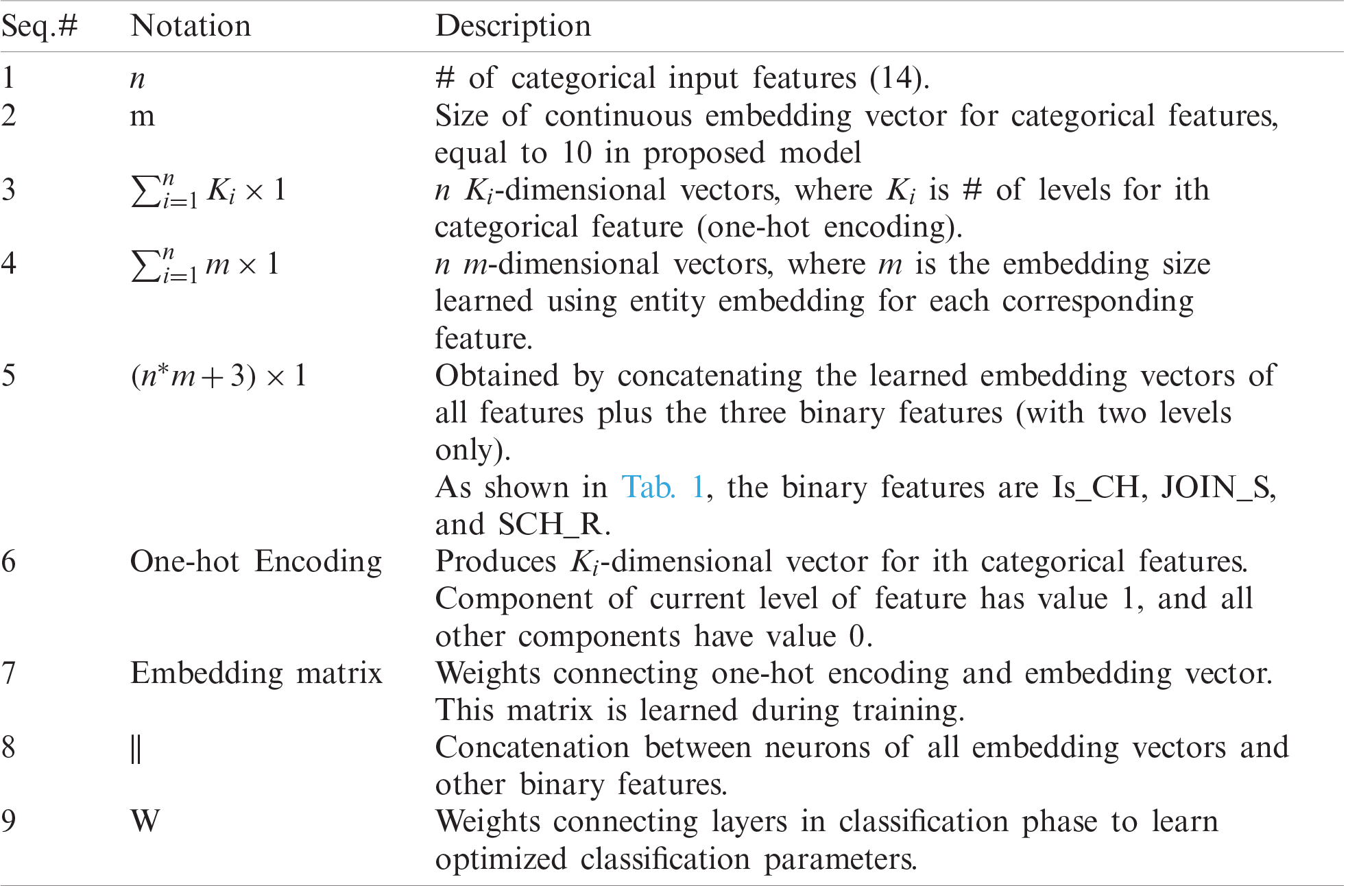
In this work, a multi-layer ANN-based architecture is proposed for a WSN intrusion detection system, as shown in Fig. 4. Tab. 2 provides details about the notation. Multi-layer ANNs (deep model) enable us to effectively learn nonlinear decision boundaries for more accurate classification. Entity embedding automatically learns a robust representation of the raw features with the help of the deep model. This work shows how to determine the optimal architecture (number of hidden layers, number of neurons in each layer, and embedding size) and investigate the optimal value for other model hyperparameters, such as the activation function and learning rate.
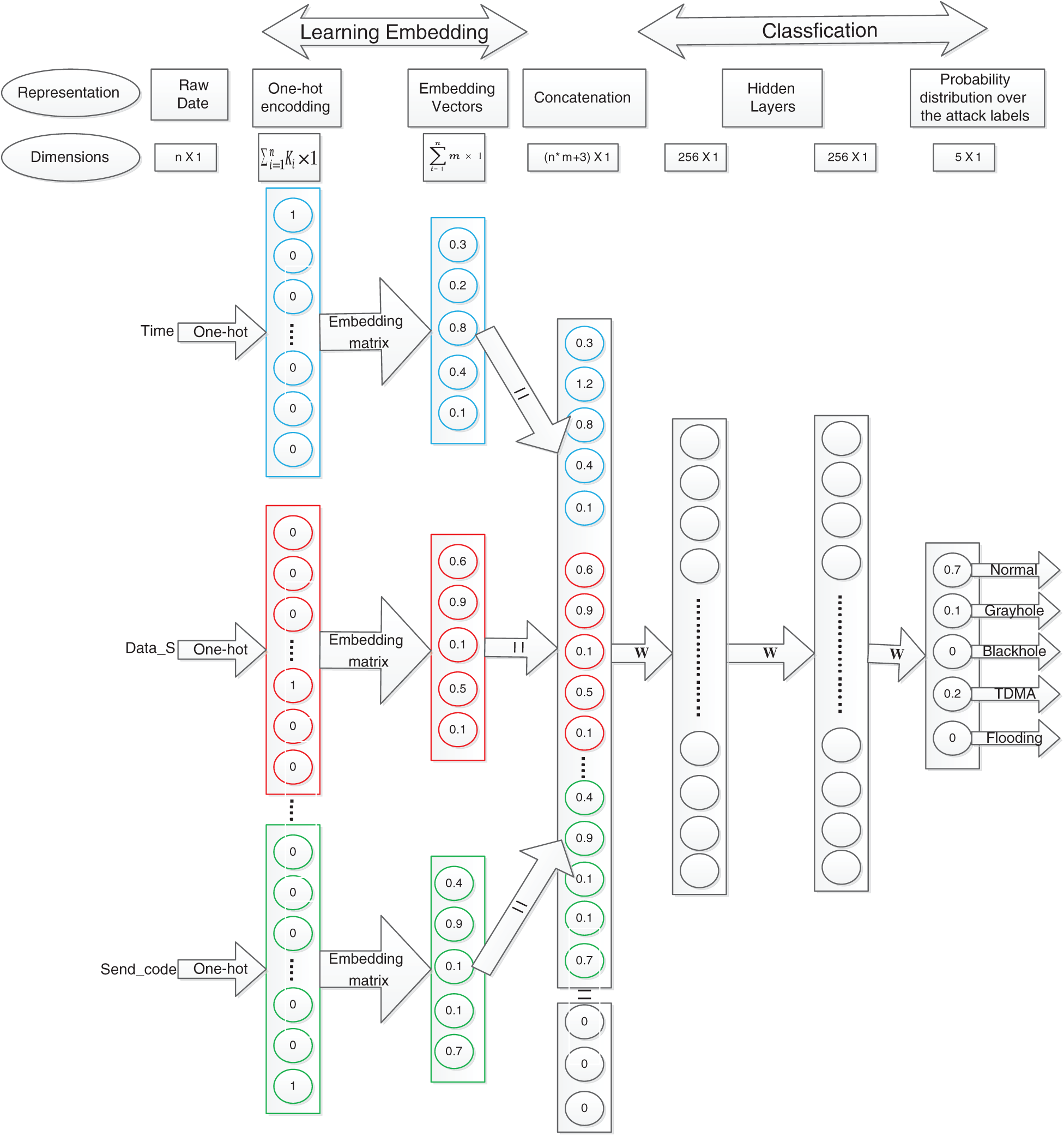
Figure 4: Proposed model architecture
As most input features for WSN intrusion detection have a limited number of levels, as shown in Tab. 1, we treat them as categorical variables. It can be noticed that the proposed architecture represents most input features using the concept of entity embedding explained above. Entity is not used directly for some input features (Who_CH, Dist_To_CH, and Consumed Energy) because the large number of unique values (# of levels) is very large, which requires the learning of a large number of parameters.
Table 2: Notation used in Fig. 4
As most input features for WSN intrusion detection have a limited number of levels, as shown in Tab. 1, we treat these as categorical variables. The proposed architecture represents the majority of the input features using the concept of entity embedding explained above. Entity embedding is not used directly for some input features (Who_CH, Dist_To_CH, and Consumed Energy) with a very large number of unique values (# of levels), which require a large number of parameters to be learned. For example, Dist_To_CH features have 13956 values, which need 139560 weights to learn an embedding vector of size 10. However, when we used entity embedding for these values, we realized that the model was over-fit. Therefore, we performed discretization (binning) on these features before passing them to the model. Discretization is accomplished by decomposing each feature into a set of bins. In the present study, we use 300, 100, and 100 bins for Consumed Energy, Dist_To_CH, and Who_CH, respectively.
Then, in the first layer, each categorical input feature is transformed to a one-hot representation. The embedding layer of size 10 is added on top of it. This layer is used to learn the embedding matrix that maps each input feature to a 10-dimensional continuous vector. This layer helps place values with similar effects near each other in the vector space, thus exposing the fundamental continuity of the data to ensure a robust representation of the input features.
Next, all learned embedding vectors and the binary features (which only include two levels) that are not required for learning its embedding are concatenated together.
Then, two fully-connected layers (256–256 neurons) are added on top of the concatenated layer and used to learn the classification weights. A softmax layer of five neurons is added on top of these layers, which helps compute the probability distribution over the attack labels. Intuition regarding the selected values of the hyperparameters (# of layers, # of neurons in each layer, embedding size, learning rate, and activation function) is related in Subsection 3.6.
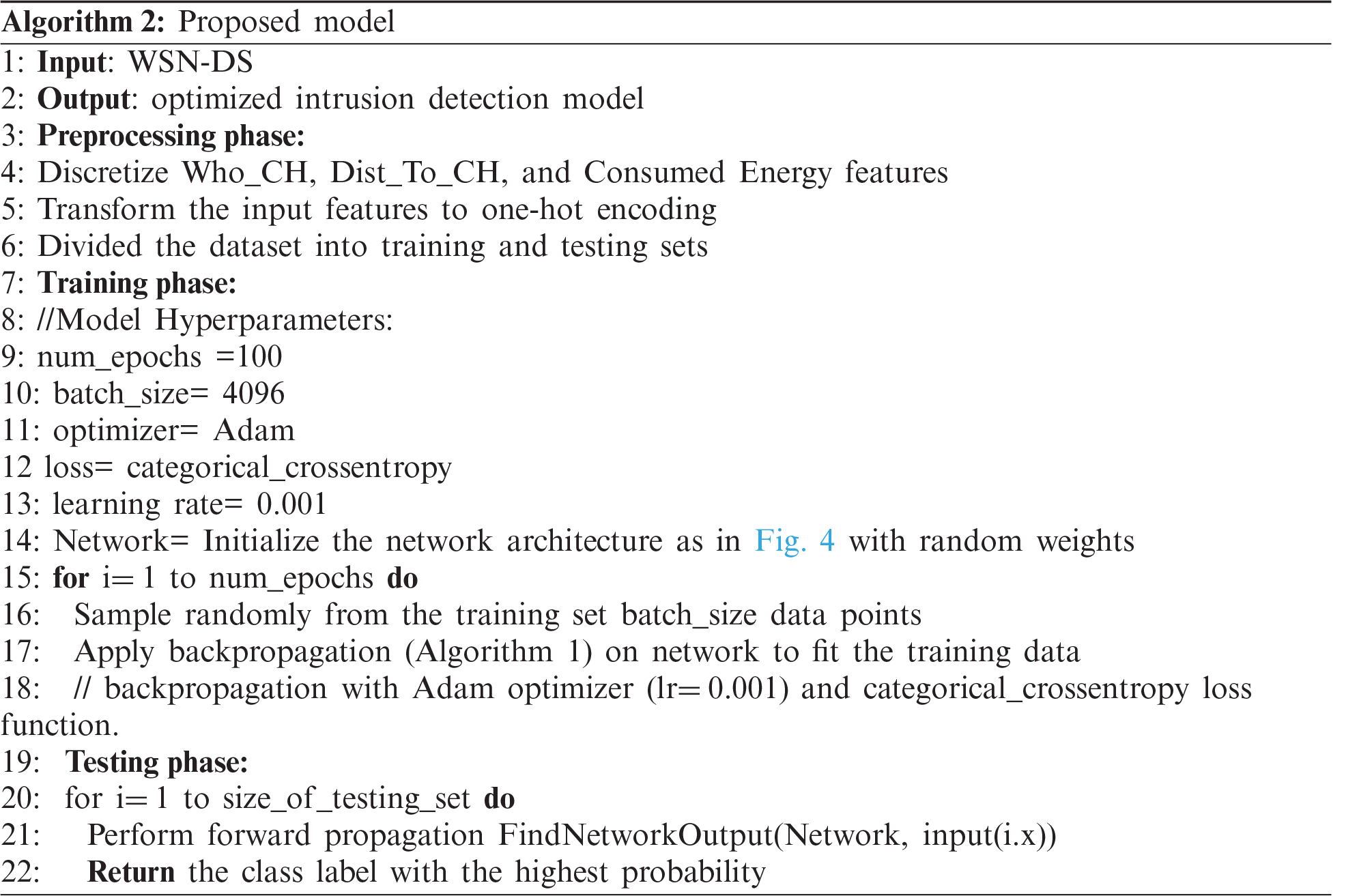
Finally, the training data are fed into the network, whose parameters (weights) are optimized using an adjusted version of stochastic gradient descent (Adam) and a backpropagation algorithm. Algorithm 2 presents the steps used to train the proposed architecture.
Different measures are available to compute evaluation scores for the classification problem. For intrusion detection systems, significant metrics include detection rate, recall, true positive rate (TPR), precision, false alarm rate/false positive rate (FPR), and F-score, defined as follows:
where TP, FP, FN, and TN are the numbers of true positives, false positives, false negatives, and true negatives, respectively.
In terms of a multi-class classification problem, the evaluation measures for all classes can be averaged as either a micro- or macro-average to obtain the general performance of a model. A micro-average is dominated by the majority class, as it treats each data point (instance) equally, whereas a macro-average gives equal weight to each class. We study an intrusion detection dataset with significantly more data points of a normal class than of abnormal classes. We use macro-averaging to prevent the majority (normal) class from dominating the performance of the model. To accelerate decision-making during model optimization and compare the proposed model to state-of-the-art methods, we use a macro-average F-score. In addition, a micro-average F-score is calculated to compare certain related work that uses a micro-average as a metric. Metrics such as recall, precision, and false-alarm rate are also used to obtain detailed information about the model’s performance.
The proposed ANN architecture has several hyperparameters that must be selected carefully, as they impact the model’s performance. A grid search technique is implemented to select the optimal combination of hyperparameters. We adjust the embedding size, number of hidden layers, and number of neurons in each layer, activation function, and learning rate.
Embedding size: Fig. 5 illustrates the dependency between different embedding sizes and the macro-avg. F-score. It can be observed that the performance was slightly improved with an increase in the embedding size, reached a peak when the embedding size was between 10 and 20, declined slightly when the embedding size was greater than 20, and was consistent until the embedding size reached 120, when it started to diminish as the embedding size increased, as the model was over-fit with a large number of weights (parameters).
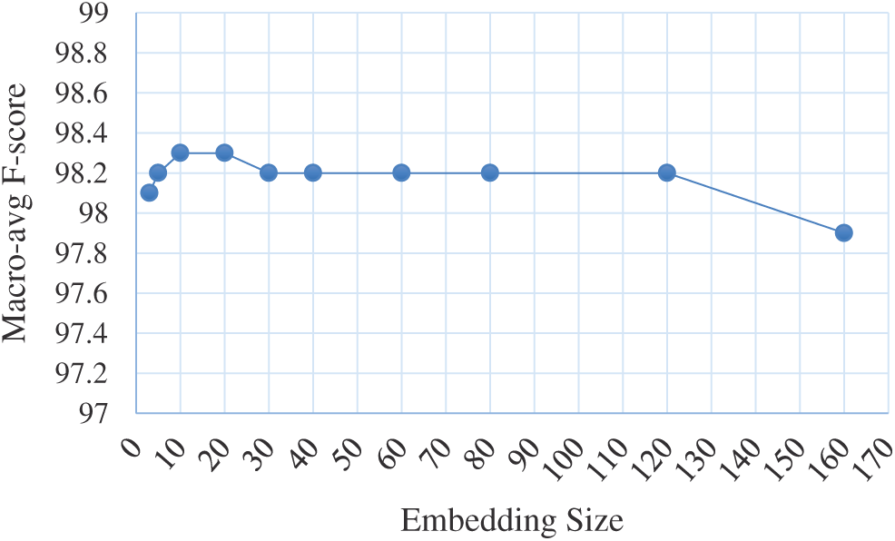
Figure 5: Dependency between embedding size and macro-avg. F-score
Number of hidden layers and number of neurons in each layer: It is important to tune these two hyperparameters concurrently to determine the best combination. Initially, only a single hidden layer spanning a range of (64, 128, 256, 512, 1025) neurons was used. Another layer was added, and the same range was applied to both layers. The process was repeated for a third layer, and it was concluded that the best macro-average F-score is achieved when there are two hidden layers, each with 256 neurons.
Activation Function: Fig. 6 shows the dependency between the type of activation function and the macro-average F-score. These functions are applied for each neuron so that the model can distinguish between the nonlinear decision boundaries of the data. Three types of activation functions, ReLU, hyperbolic tangent (tanh), and sigmoid, are usually used in ANN:
The best performance was achieved with the ReLU activation function, which is computationally more efficient, as it uses only a threshold as an input value.
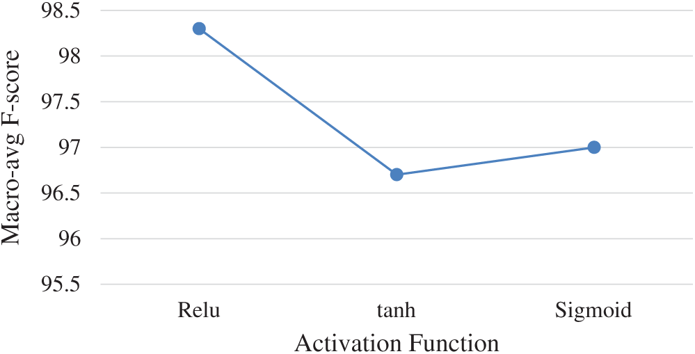
Figure 6: Dependency between activation function type and macro-avg. F-score
Learning rate: The learning rate was altered over a range of (0.0001–0.1024), with each time increment calculated by multiplying the previous value by 2. It was determined that the best macro-average F-score can be achieved when the learning rate is between 0.0008 and 0.0016. This range was further examined, and the best performance was observed to occur when the learning rate was 0.001.
Tab. 3 summarizes the tuned hyperparameters used in this work.
Subsection 4.1 presents the experimental settings used in this study. Subsection 4.2 shows the effectiveness of the proposed feature representation using entity embedding. Subsection 4.3 compares the proposed model to state-of-the-art solutions.
To ensure precision in comparisons, settings for comparative methods were those of the work in which they were proposed. The holdout technique was used to split the dataset into 60% training and 40% testing, with stratified sampling to ensure a consistent ratio of classes. Fig. 7 shows the data distribution over normal and different types of attacks for the training and test sets.
Table 3: Summary of hyperparameters used in this work
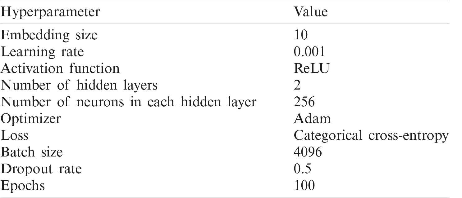
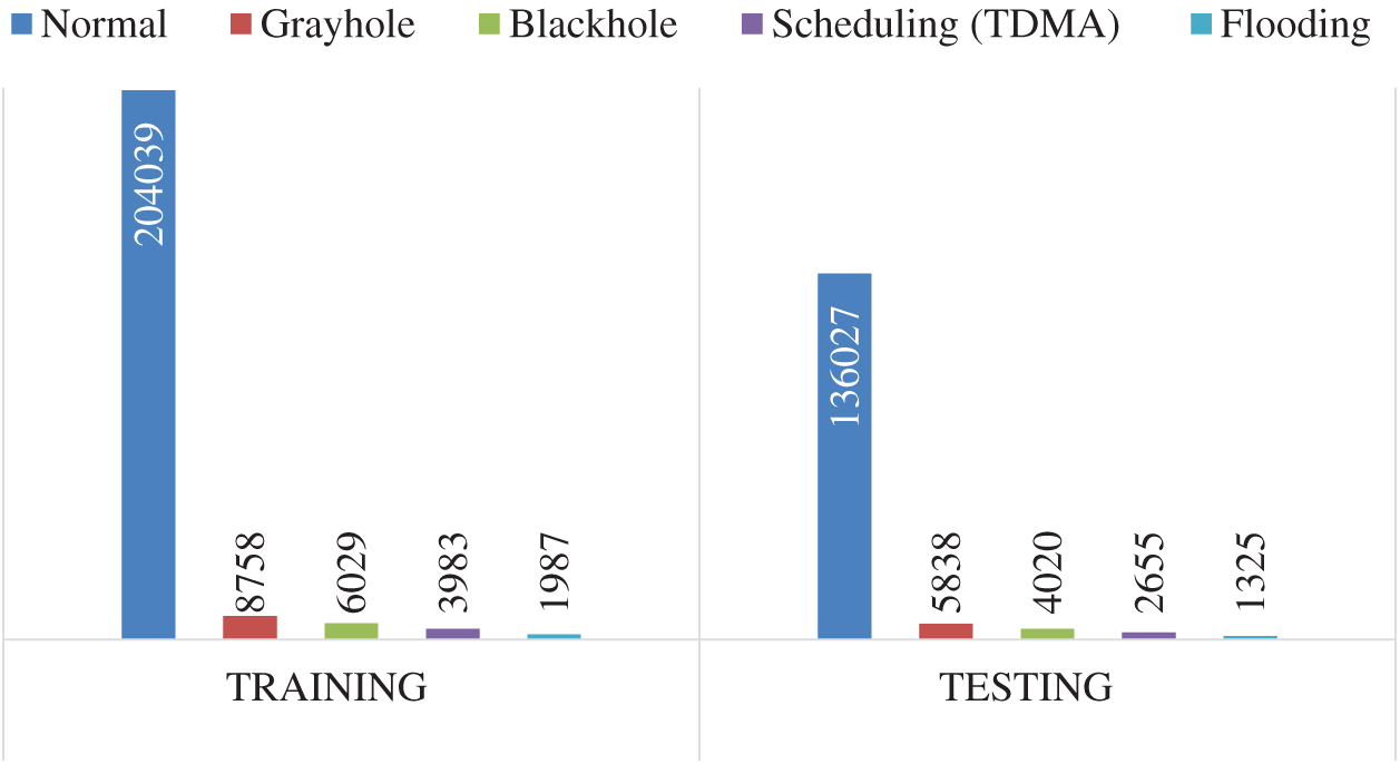
Figure 7: Data distribution over normal and different types of attacks for training and test sets
4.2 Effectiveness of Proposed Feature Representation Method
To demonstrate the power of the proposed feature representation method, its performance was compared using two approaches.
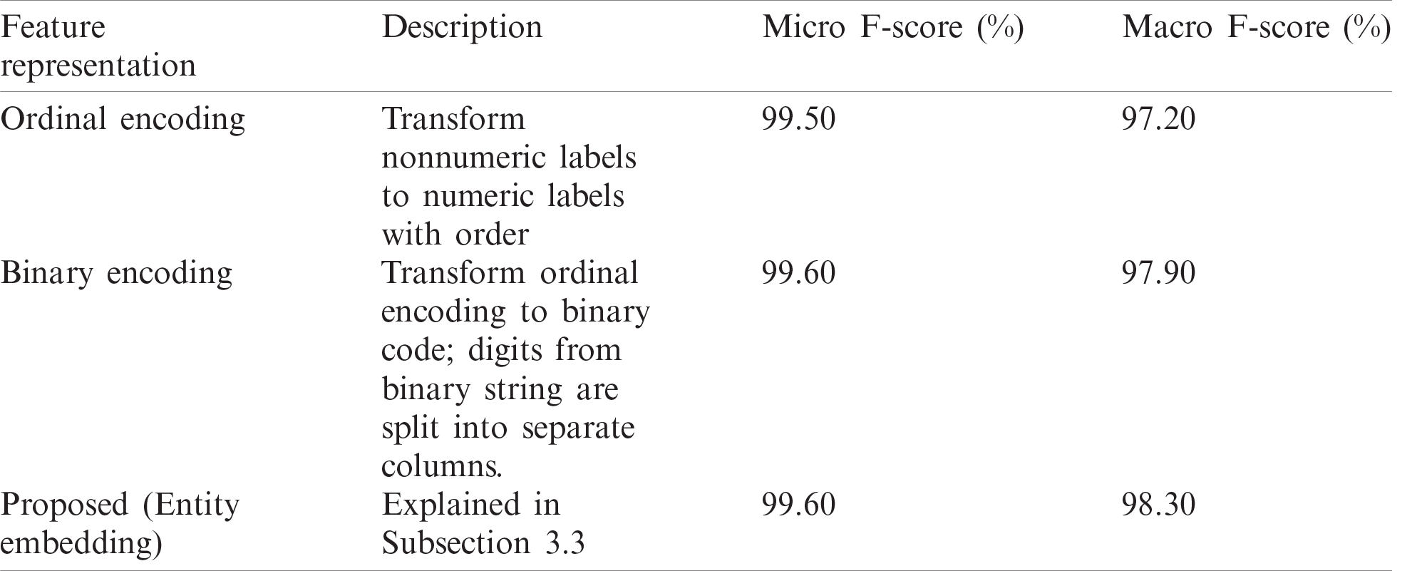
In the first approach, the feature representation methods were varied and the network architecture was unchanged. Tab. 4 compares the performance of the proposed feature representation, ordinal encoding (original feature values), and binary encoding. It is seen that the proposed feature representation outperforms other types in the macro F-score. However, binary encoding delivers performance comparable to that of the proposed method, and outperforms the state-of-the-art methods, as shown in Subsection 4.3. We believe that binary encoding performs better, as it works well with categorical features with high cardinality (# of levels).
In the second approach, the proposed method was evaluated using varying network architectures to demonstrate its effectiveness.
Table 4: Micro- and macro-avg. F-score of proposed WSN intrusion detection approaches using WSN-DS dataset
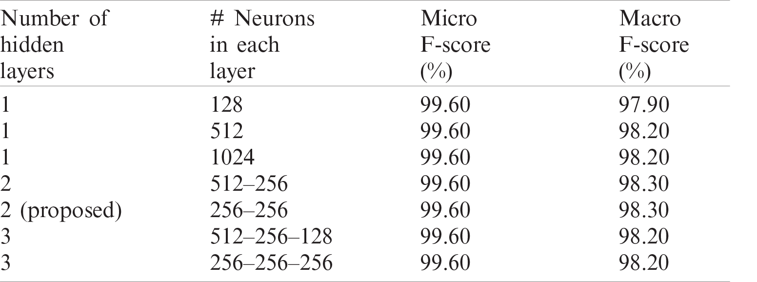
Tab. 5 presents the performance of the proposed feature representation through several network architectures. It is evident that the performance changes little as layers are added, or the number of neurons in each layer increased. This stability in performance reflects the effectiveness of the method. While 256–256 and 512–256 achieved similar performance, we selected 256–256, as it was more computationally efficient.
Table 5: Micro- and macro-avg. F-score of proposed feature representation with several network architectures
4.3 Comparison with State-of-the-Art
We show how the proposed model can outperform the state-of-the-art in terms of micro and macro F-score. It can be observed that the proposed method significantly outperforms all in terms of macro F-score, and slightly outperforms in terms of micro F-score. The slight difference in the micro-average is due to the domination of its result by the majority class (normal). Fig. 7 presents the extreme difference in the number of instances between the normal class and other abnormal classes.
Table 6: Micro- and macro-avg. F-score of proposed WSN intrusion detection approaches using WSN-DS dataset
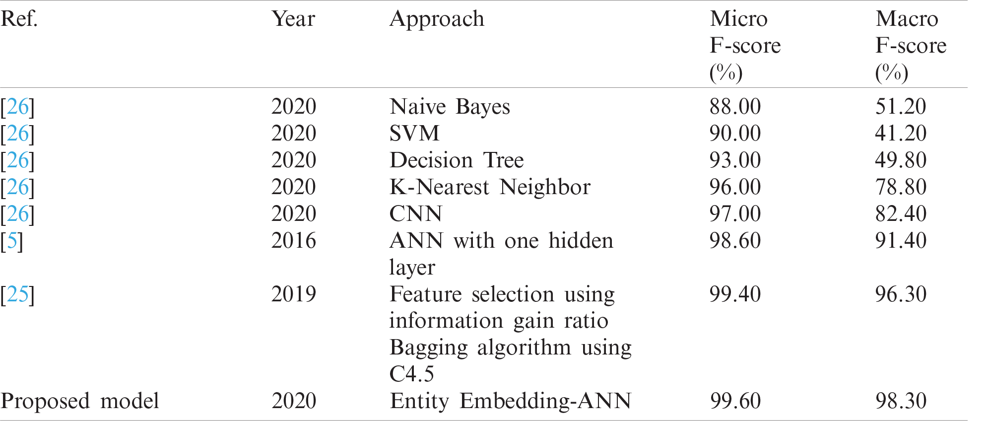
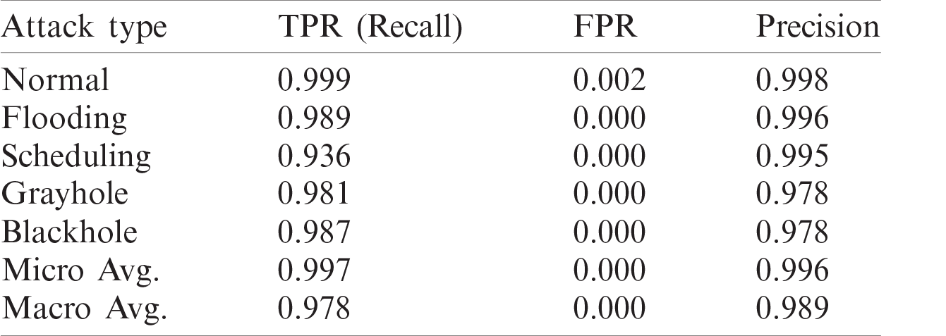
It is evident from Tab. 6 that the methods used in [5] and [25] had the highest accuracy, and the results of their solutions and that of the proposed method are given in Tabs. 7–9, respectively. The proposed method delivers better performance in terms of recall, precision, and FPR, as shown in Tabs. 6–8.
Table 7: Recall, FPR, and precision of work in [5]
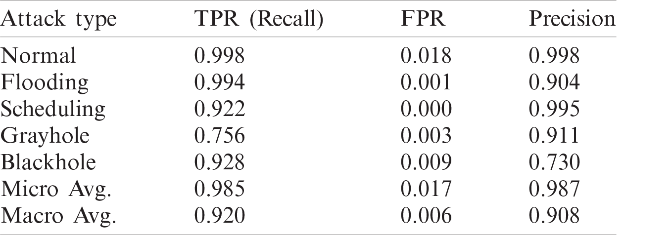
Table 8: Recall, FPR, and precision of work in [25]
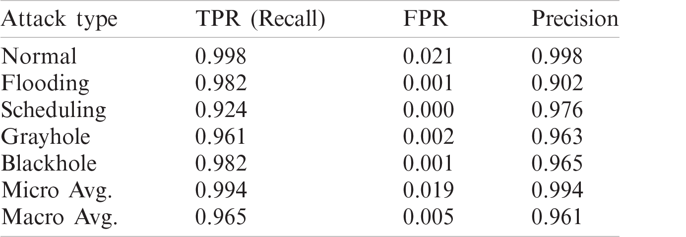
Table 9: Recall, FPR, and precision of proposed model
We proposed a deep learning architecture that uses ANNs with categorical entity embedding, and sought to demonstrate that it can produce an effective intrusion detection system for WSNs. Entity embedding was proven able to create a robust representation for raw features that can lead to better performance compared to the state-of-the-art. In future work, entity embedding representation will be used with ensemble classification instead of classical ANN to take advantage of the classification power of ensemble methods such as random forest and gradient boosted tree. This work was limited to a single dataset because of a lack of publicly available datasets collected for WSN DoS attacks. In future work, we intend to obtain another dataset to detect different DoS attacks.
Acknowledgement: This publication was supported by the Deanship of Scientific Research at Prince Sattam bin Abdulaziz University.
Funding Statement: The author received no specific funding for this study.
Conflicts of Interest: The author declares that he has no conflicts of interest to report regarding the present study.
1. Z. Feng, J. Fu, D. Du, F. Li and S. Sun, “A new approach of anomaly detection in wireless sensor networks using support vector data description,” International Journal of Distributed Sensor Networks, vol. 13, no. 1, pp. 1–14, 2017. [Google Scholar]
2. L. Breiman, “Random forests,” Machine Learning, vol. 45, no. 1, pp. 5–32, 2001. [Google Scholar]
3. T. Chen and C. Guestrin, “Xgboost: A scalable tree boosting system,” in Proc. of the 22nd Acm Sigkdd Int. Conf. on Knowledge Discovery and Data Mining, San Francisco, California, USA, pp. 785–794, 2016. [Google Scholar]
4. C. Guo and F. Berkhahn, “Entity embeddings of categorical variables,” arXiv preprint arXiv: 1604.06737, pp. 1–9, 2016. [Google Scholar]
5. I. Almomani, B. Al-Kasasbeh and M. Al-Akhras, “Wsn-ds: A dataset for intrusion detection systems in wireless sensor networks,” Journal of Sensors, vol. 2016, no. 2, pp. 1–16, 2016. [Google Scholar]
6. H. Suo, J. Wan, L. Huang and C. Zou, “Issues and challenges of wireless sensor networks localization in emerging applications,” in 2012 Int. Conf. on Computer Science and Electronics Engineering, Hangzhou, China, IEEE, vol. 3, pp. 447–451, 2012. [Google Scholar]
7. X. Chen, K. Makki, K. Yen and N. Pissinou, “Sensor network security: A survey,” IEEE Communications Surveys Tutorials, vol. 11, no. 2, pp. 52–73, 2009. [Google Scholar]
8. W. Wan, J. Chen, J. Xia, J. Zhang, S. Zhang et al., “Clustering collision power attack on rsa-crt,” Computer Systems Science and Engineering, vol. 36, no. 2, pp. 417–434, 2021. [Google Scholar]
9. Z. Shen, H. Wang, K. Liu, P. Liu, M. Ba et al., “Rp-nbsr: A novel network attack detection model based on machine learning,” Computer Systems Science and Engineering, vol. 37, no. 1, pp. 121–133, 2021. [Google Scholar]
10. N. A. Alrajeh, S. Khan and B. Shams, “Intrusion detection systems in wireless sensor networks: A review,” International Journal of Distributed Sensor Networks, vol. 9, no. 5, pp. 1–7, 2013. [Google Scholar]
11. A. D. Wood and J. A. Stankovic, “Denial of service in sensor networks,” Computer, vol. 35, no. 10, pp. 54–62, 2002. [Google Scholar]
12. H. Chen and S. Kuo, “Active detecting ddos attack approach based on entropy measurement for the next generation instant messaging app on smartphones,” Intelligent Automation & Soft Computing, vol. 25, no. 1, pp. 217–228, 2019. [Google Scholar]
13. J. Cheng, Y. Liu, X. Tang, V. S. Sheng, M. Li et al., “Ddos attack detection via multi-scale convolutional neural network,” Computers, Materials & Continua, vol. 62, no. 3, pp. 1317–1333, 2020. [Google Scholar]
14. G. Li, J. He and Y. Fu, “Group-based intrusion detection system in wireless sensor networks,” Computer Communications, vol. 31, no. 18, pp. 4324–4332, 2008. [Google Scholar]
15. Y. Maleh and A. Ezzati, “A review of security attacks and intrusion detection schemes in wireless sensor networks,” International Journal of Wireless & Mobile Networks, vol. 5, no. 6, pp. 79–90, 2013. [Google Scholar]
16. F. Geramiraz, A. S. Memaripour and M. Abbaspour, “Adaptive anomaly-based intrusion detection system using fuzzy controller,” International Journal Network Security, vol. 14, no. 6, pp. 352–361, 2012. [Google Scholar]
17. M. C. Raja and M. M. A. Rabbani, “Combined analysis of support vector machine and principle component analysis for ids,” in 2016 Int. Conf. on Communication and Electronics Systems, Coimbatore, India, IEEE, pp. 1–5, 2016. [Google Scholar]
18. G. Gowrison, K. Ramar, K. Muneeswaran and T. Revathi, “Minimal complexity attack classification intrusion detection system,” Applied Soft Computing, vol. 13, no. 2, pp. 921–927, 2013. [Google Scholar]
19. Y. Wang, Y. Shen and G. Zhang, “Research on intrusion detection model using ensemble learning methods,” in 2016 7th IEEE Int. Conf. on Software Engineering and Service Science, Beijing, China, IEEE, pp. 422–425, 2016. [Google Scholar]
20. M. C. Belavagi and B. Muniyal, “Performance evaluation of supervised machine learning algorithms for intrusion detection,” Procedia Computer Science, vol. 89, no. 9, pp. 117–123, 2016. [Google Scholar]
21. P. Aggarwal and S. K. Sharma, “Analysis of kdd dataset attributes-class wise for intrusion detection,” Procedia Computer Science, vol. 57, no. 4, pp. 842–851, 2015. [Google Scholar]
22. R. Vijayanand, D. Devaraj and B. Kannapiran, “Intrusion detection system for wireless mesh network using multiple support vector machine classifiers with genetic-algorithm-based feature selection,” Computers Security, vol. 77, no. 2, pp. 304–314, 2018. [Google Scholar]
23. F. Bao, R. Chen, M. Chang and J.-H. Cho, “Hierarchical trust management for wireless sensor networks and its applications to trust-based routing and intrusion detection,” IEEE Transactions on Network Service Management, vol. 9, no. 2, pp. 169–183, 2012. [Google Scholar]
24. J.-Y. Huang, I.-E. Liao, Y.-F. Chung and K.-T. Chen, “Shielding wireless sensor network using markovian intrusion detection system with attack pattern mining,” Information Sciences, vol. 231, no. 6, pp. 32–44, 2013. [Google Scholar]
25. R.-H. Dong, H.-H. Yan and Q.-Y. Zhang, “An intrusion detection model for wireless sensor network based on information gain ratio and bagging algorithm,” International Journal Network Security, vol. 22, no. 2, pp. 218–230, 2020. [Google Scholar]
26. P. R. Chandre, P. N. Mahalle and G. R. Shinde, “Deep learning and machine learning techniques for intrusion detection and prevention in wireless sensor networks: Comparative study and performance analysis,” in Design Frameworks for Wireless Networks, Singapore, Springer, pp. 95–120, 2020. [Google Scholar]
27. R. Collobert and S. Bengio, “Links between perceptrons, mlps and svms,” in Proc. of the Twenty-First Int. Conf. on Machine Learning, Banff, Alberta, Canada, pp. 23, 2004. [Google Scholar]
28. D. E. Rumelhart, G. E. Hinton and R. J. Williams, “Learning representations by back-propagating errors,” Nature, vol. 323, no. 6088, pp. 533–536, 1986. [Google Scholar]
29. K. Griffiths and R. Andrews, “Application of artificial neural networks for filtration optimization,” Journal of Environmental Engineering, vol. 137, no. 11, pp. 1040–1047, 2011. [Google Scholar]
 | This work is licensed under a Creative Commons Attribution 4.0 International License, which permits unrestricted use, distribution, and reproduction in any medium, provided the original work is properly cited. |