Computers, Materials & Continua DOI:10.32604/cmc.2021.016006
Article

Scattered Data Interpolation Using Cubic Trigonometric Bézier Triangular Patch

Ishak Hashim1, Nur Nabilah Che Draman2, Samsul Ariffin Abdul Karim3,*, Wee Ping Yeo4 and Dumitru Baleanu5,6,7

1Department of Mathematical Sciences, Faculty of Science and Technology, Universiti Kebangsaan Malaysia, UKM, Bangi, 43600, Selangor Darul Ehsan, Malaysia
2Department of Fundamental and Applied Sciences, Universiti Teknologi PETRONAS, Seri Iskandar, 32610, Perak Darul Ridzuan, Malaysia
3Department of Fundamental and Applied Sciences and Centre for Systems Engineering (CSE), Institute of Autonoumous System Universiti Teknologi PETRONAS, Seri Iskandar, 32610, Perak Darul Ridzuan, Malaysia
4Faculty of Science, Universiti Brunei Darussalam, Bandar Seri Begawan, BE1410, Brunei Darussalam
5Department of Mathematics, Cankaya University, Ankara, Turkey
6Institute of Space Sciences, Magurele-Bucharest, Romania
7Department of Medical Research, China Medical University Hospital, China Medical University, Taichung, Taiwan
*Corresponding Author: Samsul Ariffin Abdul Karim. Email: samsul_ariffin@utp.edu.my
Received: 18 December 2020; Accepted: 18 January 2021

Abstract: This paper discusses scattered data interpolation using cubic trigonometric Bézier triangular patches with C1 continuity everywhere. We derive the C1 condition on each adjacent triangle. On each triangular patch, we employ convex combination method between three local schemes. The final interpolant with the rational corrected scheme is suitable for regular and irregular scattered data sets. We tested the proposed scheme with 36,65, and 100 data points for some well-known test functions. The scheme is also applied to interpolate the data for the electric potential. We compared the performance between our proposed method and existing scattered data interpolation schemes such as Powell–Sabin (PS) and Clough–Tocher (CT) by measuring the maximum error, root mean square error (RMSE) and coefficient of determination (R2). From the results obtained, our proposed method is competent with cubic Bézier, cubic Ball, PS and CT triangles splitting schemes to interpolate scattered data surface. This is very significant since PS and CT requires that each triangle be splitting into several micro triangles.

Keywords: Cubic trigonometric; Bézier triangular patches; C1sufficient condition; scattered data interpolation

1  Introduction

This paper investigates scattered data interpolation using trigonometric Bézier triangular patch that has been proposed by Zhu et al. [1]. Scattered data interpolation is about the construction of a smooth surface for non-uniform set of data. It can be prescribed by a given a set of scattered data V={(xi,yi),i=1,…,n}∈R2 over a polygon domain and a corresponding set of real numbers {Zi}i=1n. Besides that, scattered data interpolation is very vital in many areas such as engineering fields, predicting rainfall and other data that needed to be measured or generated at irregular positions.

In a previous study, Saaban et al. [2] performed scattered data interpolation by using minimized sum of squares of principal curvatures. In additions, this scheme also uses geometric continuity which is G1 continuity between adjacent triangular patches to reconstruct surfaces. They applied the proposed scheme to some functions and to some real data such as soil erosion.

Butt et al. [3] proposed a scheme which exhibits the shape preserving properties by positivity, monotonicity and convexity 2D data by inserting more knots in the interval. The positivity of regular data arranged over a rectangular grid was discussed. Hussain et al. [4] proposed C1 continuity scattered data interpolation by preserving the positivity property. This scheme is modified by adding weights to the functions if the Bézier ordinates do not satisfy the derived positivity conditions.

Han [5] proposed cubic trigonometric polynomial curves with shape parameter where the order of continuity is dependent upon the knot vector (uniform or non-uniform) and the value of shape parameters. This scheme shows that the proposed scheme is closer to the control polygon than the corresponding B-spline curves. Besides that, the degree of the cubic trigonometric polynomial curves can be reduced to quadratic trigonometric polynomial curves which represent the ellipse.

Butt [6] preserved the shape of positive data by deriving sufficient conditions for the first partial derivatives and twist values by using a piecewise bi-cubic interpolant. Lamberti et al. [7] also proposed a method for the construction of C2 interpolating function. This scheme preserved the shape of curve via tension parameters. The calculation for approximation order and numerical examples is shown.

Floater [8,9] proposed another shape preserving property which is the convexity where [8] shows derivation of sufficient conditions convexity of tensor-product Bézier surfaces. The conditions focused on C1 tensor product B-spline surfaces. Unfortunately, the sufficient conditions in the form of inequalities which involved control points. Floater also defined convexity and rational convexity preservation of systems of functions. It is proven that the total positivity and rational convexity preservation are equivalent. Ali et al. [10] have constructed a new cubic Timmer triangular patch and applied it for scattered data interpolation. Based on the numerical results, their proposed scheme is better than the existing schemes in term of higher R2 and smaller SMSE and maximum error, however, their scheme took longer computational time to generate the results. Meanwhile Draman et al. [11] have constructed scattered data interpolation scheme by using rational quartic spline with three parameters. Karim et al. [12] have constructed new cubic Bézier-Like triangular patches with three parameters for scattered data interpolation. From numerical results, their proposed scheme is better than Radial basis functions (RBFs) scheme such as thin plate spline, gaussian etc.

The aim of this paper is to apply scattered data interpolation with trigonometric function which is cubic trigonometric Bézier. To our knowledge, this is the first study that applies trigonometric Bézier triangular for scattered data interpolation. We summarize the main advantages of the proposed scheme as follows:

a) The proposed scattered data interpolation uses cubic trigonometric Bézier with three parameters meanwhile Ali et al. [10], Draman et al. [11] and Karim et al. [12] have used different types of rational interpolants.

b) Our scheme only needs to triangulate the data one time. Meanwhile, Powell–Sabin (PS) and Clough–Tocher (CT) schemes needed to split the macro triangles into several micro triangles for each triangle. This will increase computation time to construct the final interpolating surface.

This paper is organized as follows: Section 2 discusses trigonometric Bézier triangular patches with three shape parameters. Section 3 states the properties of cubic trigonometric Bézier. Section 4 discusses the scattered data interpolation. Section 5 presents the numerical results including comparison with existing schemes. Conclusion and future work are given in Section 6.

2  Trigonometric Bézier Triangular Patch with Three Shape Parameters

Trigonometric Bézier triangular patches is constructed by Zhu et al. [1]. The trigonometric Bézier triangular patches are defined as follows:

Definition 1. Let α,β,γ∈[2,+∞), given control points Pijk∈R3 (i,j,k∈N,i+j+k=3), and a domain triangle D={(u,v,w)∣u+v+w=π/2,u≥0,v≥0,w≥0} in which (u,v,w) are barycentric coordinates of the points in D. We call

R(u,v,w)=∑i+j+k=3Ti,j,k3(u,v,w;α,β,γ)Pi,j,k(u,v,w)∈D(1)

the trigonometric Bézier-Like patch over triangular domain with three exponential shape parameters α,β,γ.

Noted that, Ti,j,k is the basis function that stated in Definition 2

Definition 2. Let α,β,γ∈[2,+∞) for D={(u,v,w)∣u+v+w=π/2,u≥0,v≥0,w≥0} the following ten functions are defined as trigonometric Bézier Triangular patches.

T1,0,23(u,v,w;α,β,γ)=cosvsinu(1−cosw)[1+cosw−(1−cosw)γ−1cosw](2)

Properties of Cubic Trigonometric Bézier Triangular Patches

From the definition of the basis function of trigonometric triangular patches, the list below is important properties of the basis [1].

a) Affine invariance and convex hull. The basis function have the properties of partition of unity and nonnegativity, so its simply corresponding that cubic trigonometric Bézier has

b) Geometric property at the corner points. Direct computation such as R(π/2,v,w)=P3,0,0R(u,π/2,w)=P0,3,0R(u,v,π/2)=P3,0,0 corner.

c) Corner points tangent plane.

d) Boundary property.

e) Shape adjustable property.

3  Scattered Data Interpolation

In this section, we will discuss the constrution of a smooth surface for given a set of scattered data V=(xi,yi,zi),i=1,2,…,N with corresponding a set of real numbers zi=F(xi,yi),i=1,2,…,N. We wish to reconstruct a surface which has C1 continuity everywhere. Throughout this section, we have adopted the main ideas from [11–15].

Local scheme

This scheme comprises of the convex combination of three local schemes P1,P2 and P3 and is defined as

R(u,v,w)=vwP1+uwP2+uvP3vw+uw+uv,u+v+w=1(3)

R(u,v,w)=u2v2P1+v2w2P2+u2w2P3u2v2+v2w2+u2w2,u+v+w=1(4)

or

where the local scheme P1,P2,P3 is derived and replaces the inner ordinates in the proposed method as show in Fig. 1.

For inner ordinates, we have employed the cubic precision that was proposed by Foley et al. [15] while Goodman et al. [14] methods are used to calculate the boundary ordinates for each triangle. The vertices V1,V2 and V3 with barycentric coordinates (1, 0, 0), (0, 1, 0) and (0, 0, 1) respectively meanwhile e1,e2 and e3 are direction vectors which are (0, −1, 1), (1, 0, 1) and (−1, 1, 0) respectively.

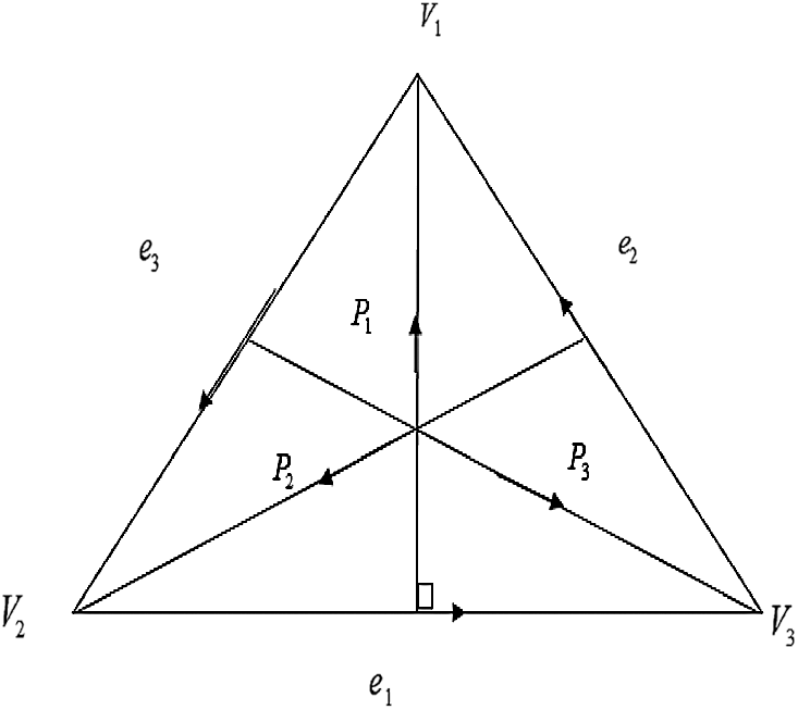
Figure 1: Directional derivatives

Let the directional derivatives along e3 and e2 at V1 be

δRδe2(V1)=(δxδv−δxδu)Fx(V1)+(δyδv−δyδu)Fy(V1)=(x1−x3)Fx(V1)+(x1−x3)Fy(V1)(5)

δRδe3(V1)=(δxδv−δxδu)Fx(V1)+(δyδv−δyδu)Fy(V1)=(x2−x1)Fx(V1)+(x2−x1)Fy(V1)(6)

Then, applying directional derivative into (3), yields

δRδe2(V1)=(2+α)(P300−P201)(7)

δRδe3(V1)=(2+α)(P210−P300)(8)

From (5) until (8), we get

P201=P300−1(2+α)[(x1−x3)Fx(V1)+(y1−y3)Fy(V1)](9)

P210=P300+1(2+α)[(x2−x1)Fx(V1)+(y2−y1)Fy(V1)](10)

Other directional derivatives along e1,e3 at V2 and e1,e2 at V3 are given as follows:

Now, we need to calculate the inner ordinates for each triangle. In order to calculate inner ordinates b111k,k=1,2,3, we have adopted Foley et al. [15] to achieve cubic precision. Since the proposed scheme is cubic degree, then cubic precision will produce surface up to degree three [15].

The inner ordinate b1111 is given as [11]

Meanwhile, inner ordinate c1111 is given by [6]

The remaining inner ordinates are obtained by symmetry [11].

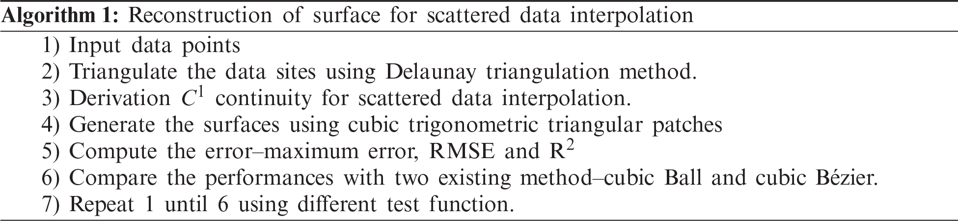
Now, we establish the algorithm that can be used for surface reconstruction using the proposed scheme.

4  Results and Discussion

In this subsection, we discuss the performance of our proposed method by measuring 36,65 and 100 data points. Besides that, we also compare the maximum error, root mean square error (RMSE) and coefficient determination (R2). All numerical simulations are done by using MATLAB version 2019 installed on Intel® CORE™ i5-2410M CPU@2.30 GHz. Four tested functions are chosen by sampling the points to 36, 65 and 100.

•   Franke’s exponential function.

where

•   Saddle function

•   Cliff function

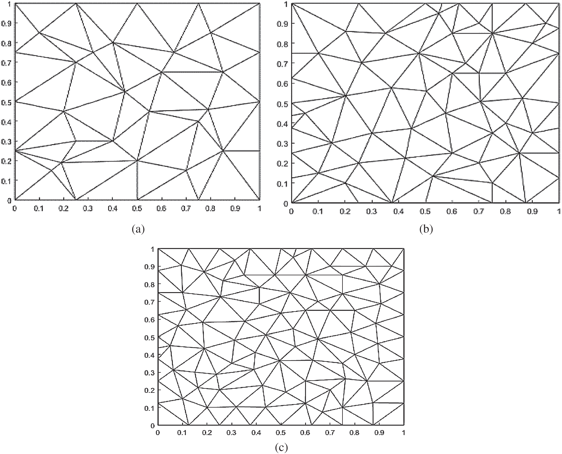
Figure 2: Delaunay triangulations. (a) Delaunay triangulation: 36 data points. (b) Delaunay triangulation: 65 data points. (c) Delaunay triangulation: 100 data points

•   Gentle function

Fig. 2 shows Delaunay Triangulation of 36, 65 and 100 data points with domain of [0,1]×[0,1]. Fig. 3 until Fig. 4 shows surface interpolation for 36 and 65 data points.

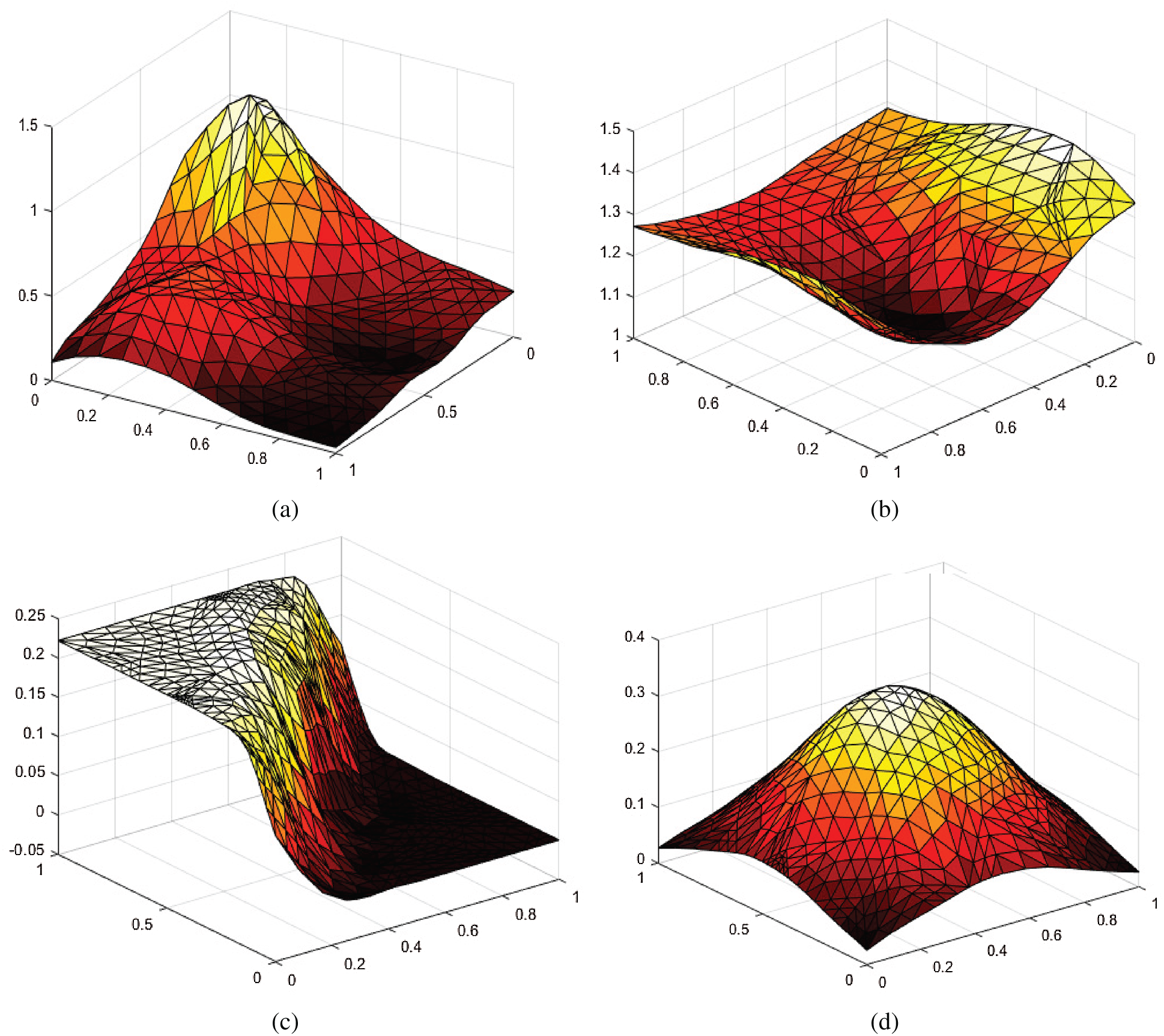
Figure 3: Surface interpolation for 36 data points. (a) H(x,y) (b) P(x,y) (c) R(x,y) (d) F(x,y)

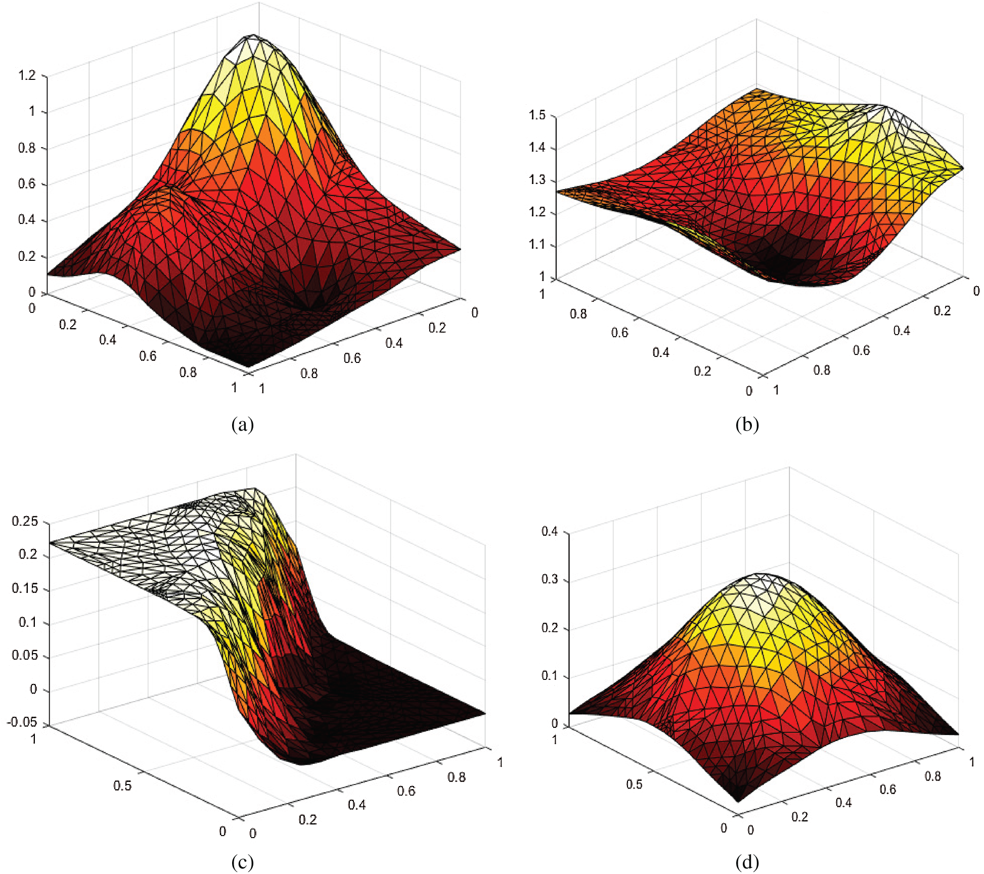
Figure 4: Surface interpolation for 65 data points. (a) H(x,y) (b) P(x,y) (c) R(x,y) (d) F(x,y)

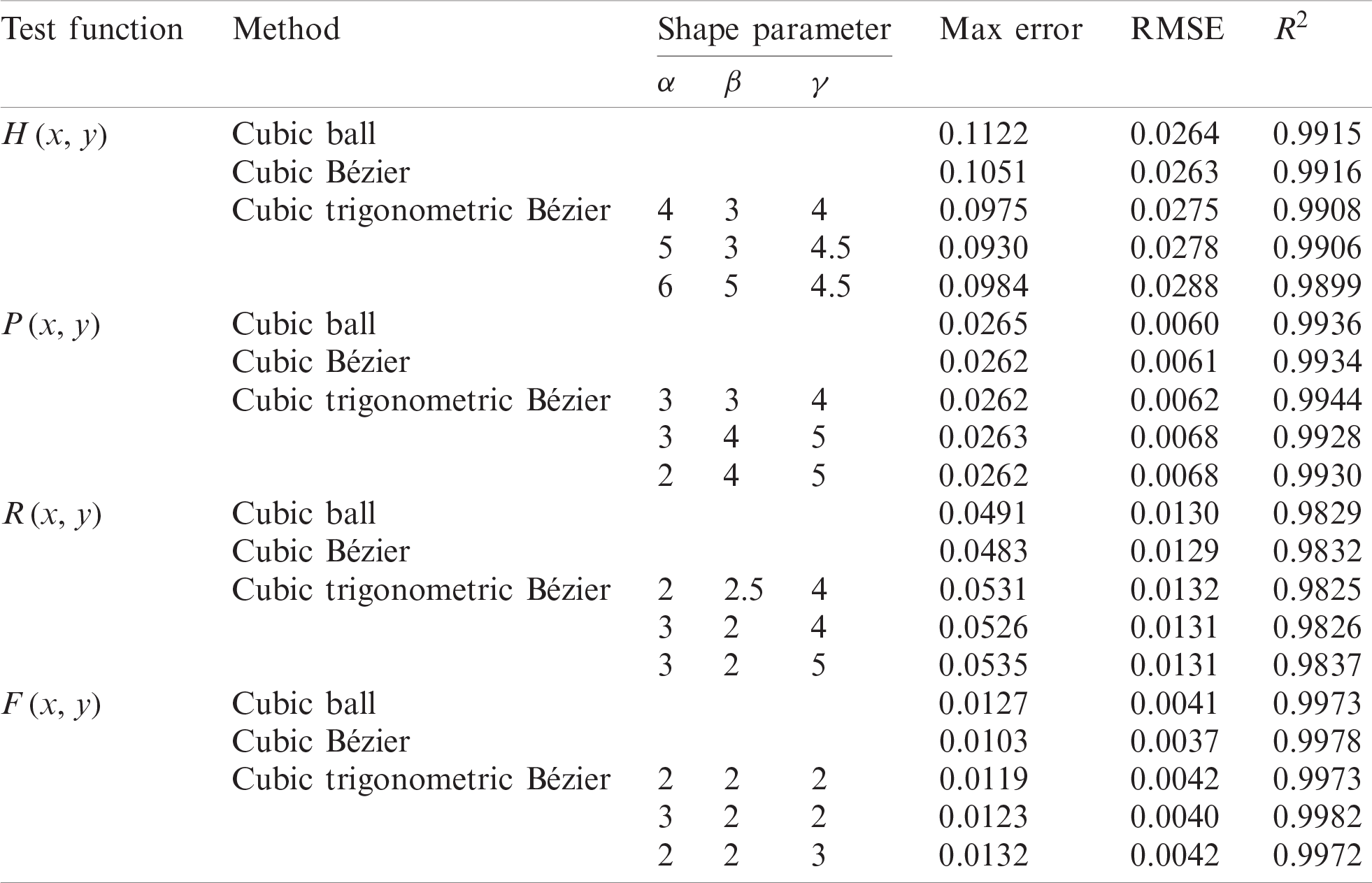
Tabs. 1–3 shows numerical result for error measurement for 36, 65 and 100 data points.

Tabs. 1–3 show numerical results for 36, 65 and 100 data points. We can see in Tabs. 1–3, the proposed scheme is on par with two established schemes i.e., Goodman et al. [14] and Karim et al. [16].

Now, we compare the performance between the proposed scattered data interpolation scheme against two well-known scattered data interpolation methods i.e., C1 Cubic Clough–Tocher (CT) and C1 quadratic Powell–Sabin (PS) schemes (Schumaker [17–18]). Tabs. 4 and 5 summarize all results. Overall, the proposed scheme is also on par with PS and CT schemes. However, in term of RMSE, both PS and CT are better than the proposed scheme. This is understandable since, both PS and CT have refining the macro triangles into many macro triangles. This will reduce the interpolation error but at a cost, CPU time will be increased. All schemes are equivalent good in term of R2. Figs. 5, 6 show the PS and CT splitting schemes. PS schemes tend to produce not smooth surfaces around the corner compared with the proposed scattered data interpolation scheme.

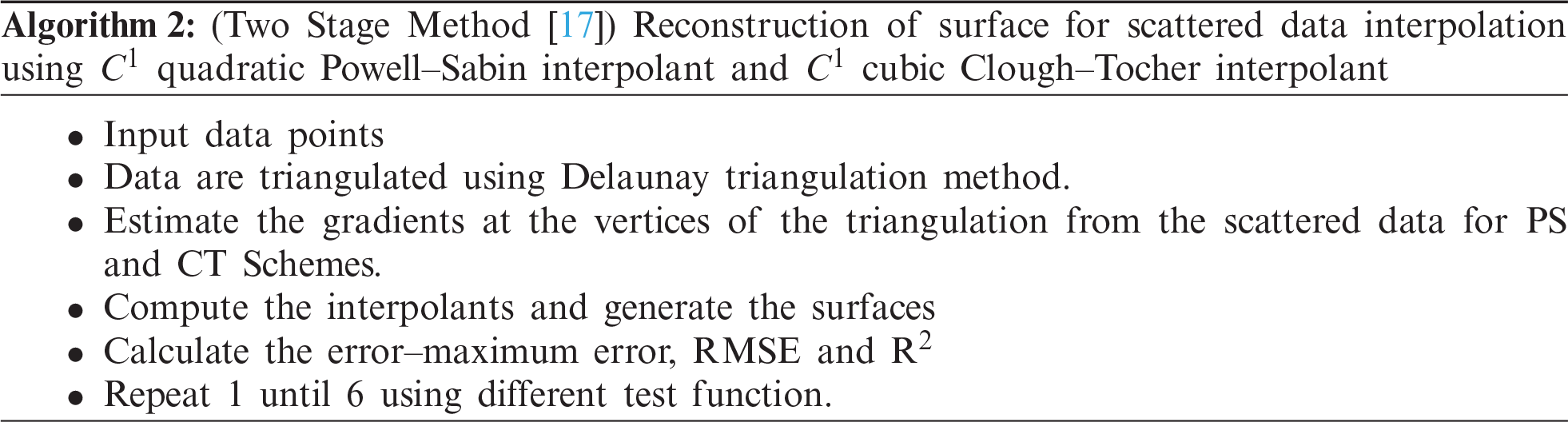
Table 1: Error measurement for 36 data points

Our final example in this study is to apply the proposed scheme to visualize real scattered data obtained from Ali et al. [19] and Gilat [20]. The electric potential V around a charged particle is given by:

where ε0=8.8541878×10−12CNm2 is the permittivity constant, r is the distance from the particle in meters and q is the magnitude of the charge in Coulombs. The electric potential at a point due to two particles is given as

where q1,q2,r1 and r2 are the charges of the particles and the distance form the points to the corresponding particles, respectively. Two particles with a charge is q1=2×10−10C and q1=3×10−10C. Noted that r1=(x+0.25)2+y2 and r2=(x−0.25)2+y2.

Fig. 7 shows the Delaunay triangulation for electric potential, and Fig. 8 shows surface interpolant using the proposed scheme.

Table 2: Error measurement for 65 data points

Table 3: Error measurement for 100 data points

Table 4: Errors using PS and CT schemes

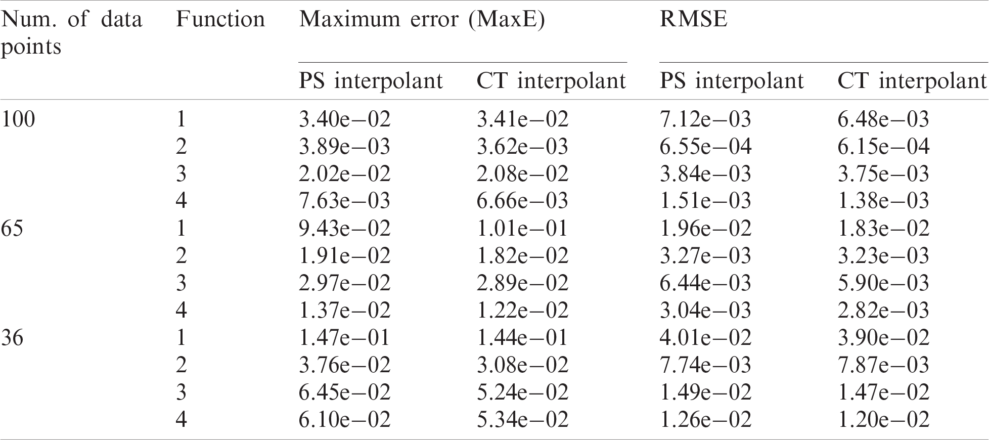
Table 5: R2 values for PS and CT

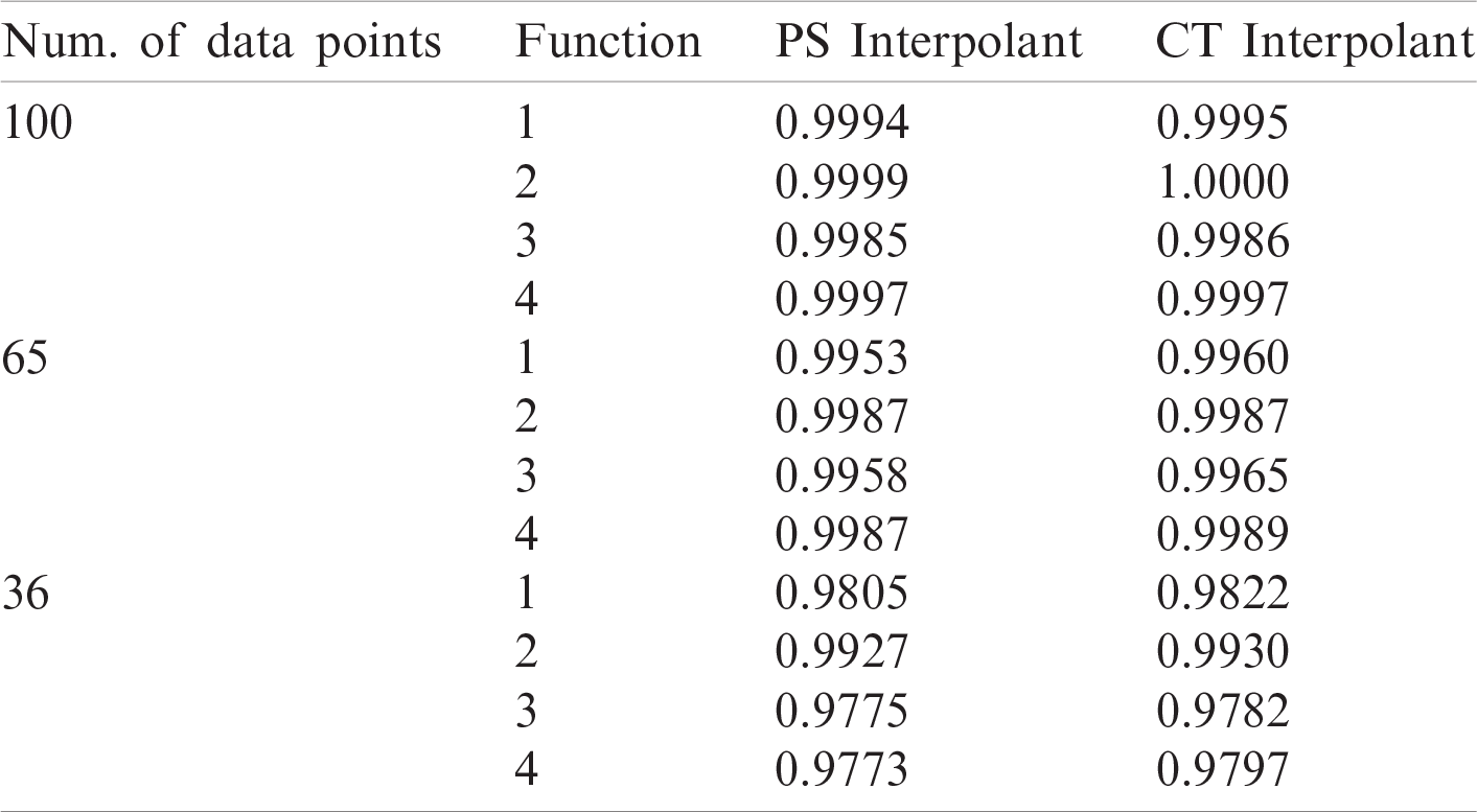
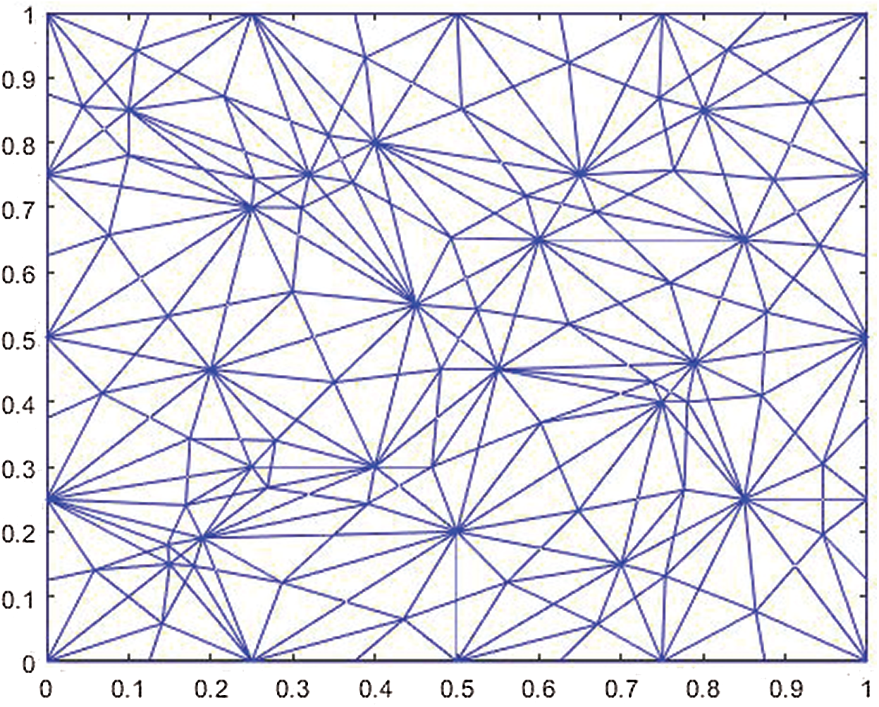
Figure 5: Powell–Sabin split

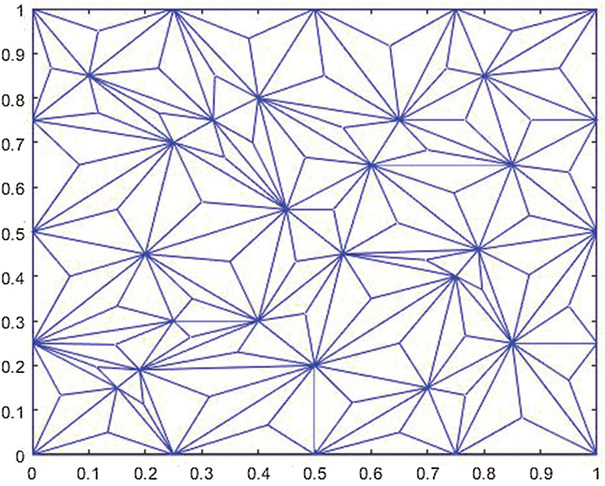
Figure 6: Clough–Tocher split

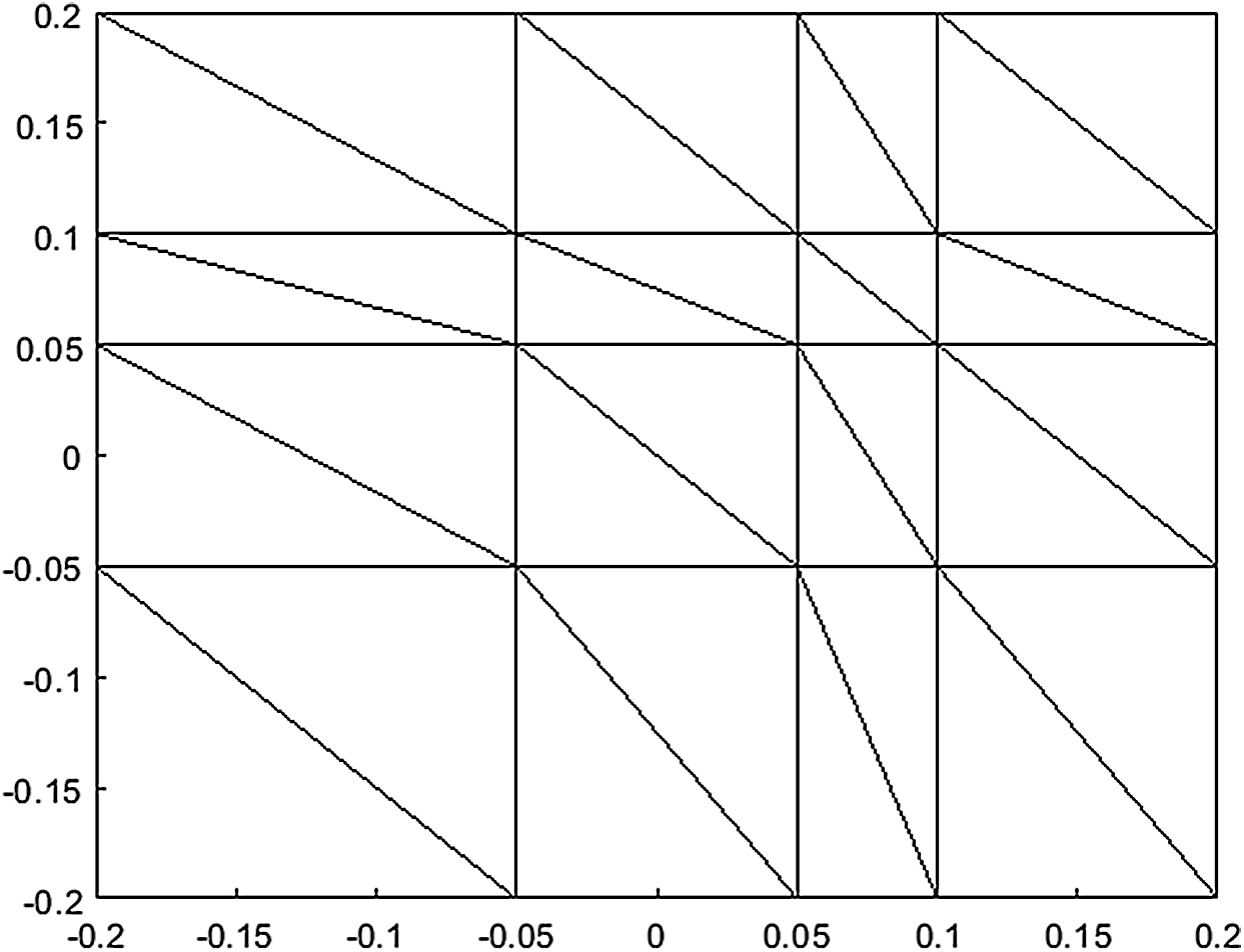
Figure 7: Delaunay triangulation

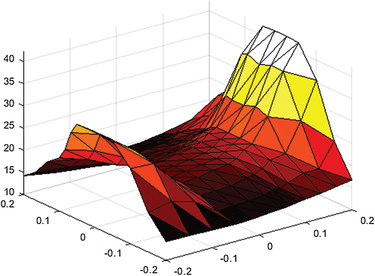
Figure 8: Surface interpolation

5  Conclusion

This paper discusses scattered data interpolation by using cubic trigonometric Bézier triangular patches initiated by Zhu et al. [1]. Sufficient condition for C1 continuity on each adjacent triangle is developed by using cubic precision method. An efficient algorithm is presented. We test the proposed scheme by using four well-known tested functions. We compare the performance against some established schemes such as Goodman et al. [14], Karim et al. [16] and Powell–Sabin (PS) and Clough–Tocher (CT) split schemes. From error analysis, we found that the proposed scheme is on par and for all data sets, we achieve higher R2 values. Finally, we test the proposed scheme to interpolate real scattered data set. For future research, we can apply the proposed scheme for shape preserving interpolation such as positivity and convexity. The proposed scheme also can be applied for constrained surface modeling above, below or between two planes as discussed in Karim et al. [21].

Funding Statement: This research was fully supported by Universiti Teknologi PETRONAS (UTP) and Ministry of Education, Malaysia through research grant FRGS/ 1/2018/STG06/UTP/03/1/015 MA0-020 (New rational quartic spline interpolation for image refinement) and UTP through a research grant YUTP: 0153AA-H24 (Spline Triangulation for Spatial Interpolation of Geophysical Data).

Conflicts of Interest: The authors declare that they have no conflicts of interest to report regarding the present study.

This work is licensed under a Creative Commons Attribution 4.0 International License, which permits unrestricted use, distribution, and reproduction in any medium, provided the original work is properly cited.