Computers, Materials & Continua DOI:10.32604/cmc.2021.017510
Article

Assessing the Performance of Some Ranked Set Sampling Designs Using HybridApproach

Mohamed. A. H. Sabry1,*, Ehab M. Almetwally2, Hisham M. Almongy3 and Gamal M. Ibrahim4

1Faculty of Graduate Studies for Statistical Research, Cairo University, Giza, 12613, Egypt
2Faculty of Business Administration, Delta University of Science and Technology, Mansoura, 35511, Egypt
3Department of Statistics, Delta University for Science and Technology, Mansoura, Egypt
4High Institute for Management Sciences, Belqas, 35511, Egypt
*Corresponding Author: Mohamed. A. H. Sabry. Email: mohusss@gmail.com
Received: 01 February 2021; Accepted: 08 March 2021

Abstract: In this paper, a joint analysis consisting of goodness-of-fit tests and Markov chain Monte Carlo simulations are used to assess the performance of some ranked set sampling designs. The Markov chain Monte Carlo simulations are conducted when Bayesian methods with Jeffery’s priors of the unknown parameters of Weibull distribution are used, while the goodness of fit analysis is conducted when the likelihood estimators are used and the corresponding empirical distributions are obtained. The ranked set sampling designs considered in this research are the usual ranked set sampling, extreme ranked set sampling, median ranked set sampling, and neoteric ranked set sampling designs. An intensive Monte Carlo simulation study is conducted using Lindley’s approximation algorithm to compute the different designs’-based estimators. The study showed that the dependent design “neoteric ranked set sampling design” is superior to other ranked set designs and the total relative efficiency is higher than the other designs’ total relative efficiency.

Keywords: Goodness of fit; ranked set sampling; Weibull distribution; Bayesian estimation; Lindley’s approximation; neoteric; ranked set sampling design

1  Introduction

Ranked set sampling (RSS) designs were first established in [1], to find a more efficient method to estimate the mean pasture yields. Since then, several modifications were considered to provide more efficient estimators and to reduce the errors in the ranking, see [2], and subsequently it will be possible to have better fits to the data under consideration. Extreme ranked set sampling (ERSS) design was introduced in [3], as the first modification of RSS, while [4] introduced another modification called median ranked set sampling (MRSS) design. The moving extreme ranked set sampling (MERSS) design was proposed in [5], while [6] introduced the double ranked set sampling (DRSS) design and proved that the population mean estimated using DRSS samples is more accurate and precise than those estimated with RSS and simple random sampling (SRS) designs. Later on, [7] suggested the multistage ranked set sampling (MSRSS) design as a generalization of the DRSS design. In [8] Zamanzade investigated a new ranked set sampling design with a dependence structure called neoteric ranked set sampling (NRSS) design and showed that NRSS based estimators are superior to the independent RSS based estimators. Moreover, two-stage NRSS designs were proposed in [9], where they showed that five different sampling designs based on NRSS outperform RSS and NRSS designs. The likelihood estimation of distribution parameters using DRSS, NRSS, and DNRSS designs were proposed by [10,11], and showed that the proposed likelihood estimators provide similar results as when estimating population means and variances using these designs.

This paper aims to use goodness-of-fit (GOF) tests and indices together with Markov chain Monte Carlo (MCMC) simulations to assess the performance of four ranked set sampling designs, RSS, ERSS, MRSS, and NRSS designs. GOF analysis includes Kolmogorov–Sminarov test, the Akiki information criterion (AIC), the corrected Akiki criterion (CAIC), the Hanan Quatine information criterion (HQIC), and Schwarz Bayesian information criterion (BIC) indices.

Goodness-of-fit (GOF) tests are utilized in many areas of research where they are used to verify the distance between the theoretical distribution and the empirical distribution of a given set of data. These tests determine how well the distribution under study fits the data set in use. They can be applied to test the simple hypothesis which completely specifies the model, and composite hypotheses where only the name of the model/distribution is stated but not its parameters as the parameters are estimated from the data. When testing GOF using SRS samples, tests based on the empirical distribution function (EDF) are usually used. These tests include the Kolmogorov–Smirnov (KS) and Cramer–Von Mises (CVM) GOF tests discussed in [12] who gave a practical guide to GOF tests using statistics based on EDF. A comprehensive survey of GOF tests based on SRS can be found in [13], while when using RSS samples, these tests can be obtained simply by replacing the SRS EDF with the unbiased RSS EDF see [14]. GOF indices such as AIC, CAIC, HQIC, and BIC are used for model selection and provide fair comparisons between different distribution candidates.

The rest of the paper is organized as follows: Section 2 is devoted to a simple introduction to the Weibull distribution, while Section 3 will introduce the four RSS designs used in the research. In Section 4, Bayesian analysis is considered for all designs including the SRS design, and in Section 5, the hybrid analysis and numerical study are investigated. Finally, the paper is concluded in Section 6.

2  The Weibull Distribution

The Weibull distribution, which is considered one of the widely used lifetime distributions in reliability engineering, was introduced in [15]. It is a flexible distribution that can take on the characteristics of other types of distributions, based on the value of the shape parameter. The cdf, pdf, and the quantile functions of the Weibull distribution are given by

F(x;α,β)=1−e−αxβ, (1)

f(x;α,β)=αβxβ−1e−αxβ, (2)

and

Q(u)=[−ln(1−u)α]1β, (3)

respectively, where x>0, α>0, β>0 and 0<u<1. Fig. 1 shows some pdf structures for the Weibull distribution at selected values of the scale and shape parameters.

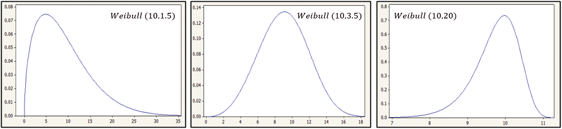
Figure 1: Weibull probability density function for several shape parameter values

3  Different Ranked Set Sampling Designs

In this section, we will discuss the ranked set sampling designs considered in this research, and we will assume for simplicity purposes that the derivations and computations needed are made in one cycle (c=1).

3.1 RSS Design

The RSS algorithm according to [16] is described as (i) select m2 units randomly from the target population with cumulative distribution function (cdf) F(x;θ) and probability density function (pdf) f(x;θ). (ii) Allocate the m2 selected units as randomly as possible into m sets, each of size m. (iii) Rank the units within each set without yet knowing any values for the variable of interest. The ranking can be based on personal or professional judgment or done on a concomitant variable correlated with a variable of interest. (iv) Choose a sample for actual quantification by including the smallest ranked unit in the first set, the second smallest ranked unit in the second set, the process continues in this way until the largest ranked unit is selected from the last set. (v) Repeat Steps (i) through (iv) for c cycles to obtain a sample of size n=mc.

3.2 ERSS Design

The first RSS modification proposed in [3] was used to estimate the population's mean only using the maximum or minimum ranked units from each set. The process of selecting an ERSS sample is as follows: (a) Repeat steps (i) through (iii) in RSS design. (b) According to the set size, if it is even or odd, the selection method may be changed. If the set size m is even, select the lowest-ranked unit of each set from the first m2 sets and select the largest ranked unit of each set from the other m2 sets. If the set size is odd, select the lowest-ranked unit from the first m−12 sets, the median unit of the m2th set, and the largest ranked unit from the remaining m−12 sets. (c) Repeat the above steps r times to obtain a sample of size n=mr.

3.3 MRSS Design

It was introduced by [4] to estimate the population mean effectively. It was shown that the MRSS provides an efficient and unbiased mean estimator when the underlying distribution is symmetric. The scheme of MRSS is first as the usual RSS. The process is as follows, (a) repeat steps (i) through (iii) in RSS design. (b) If the set size m is odd, select the median element of the set; otherwise, select the (m2) ranked unit from the first m2 sets and the from the remaining m2 sets select the (m+22) ranked unit. (c) Repeat the above steps r times to obtain a sample of size n=mr.

3.4 NRSS Design

The following process describes the NRSS design proposed by [8]: (a) Select m2 random units from the target population and rank the m2 sample units based on some preestablished ordering criterion. (b) Select the sample unit ranked in position [(i−1)m+l]th for the final sample for i=1,…,m, where if m is odd, l=m+12, and if m is even, l=m+22 for odd i and l=m/2 for even i. (c) Steps (a) and (b) can be repeated r times to obtain a final sample of size n=mr.

4  Bayesian Estimation

In this section, Bayes estimators of Weibull distribution parameters α and β are obtained under the assumption that α and β are independent random variables distributed with Jeffery's prior distributions as non-informative priors with densities given, respectively, by

Pα(α)∝1α,α>0, (4)

and

Pβ(β)∝1β,β>0, (5)

It is to be noticed that in the current study, we will use the squared error loss function to derive the Bayesian estimators of both α and β.

4.1 Estimation Based on SRS Design

Assume that {xi, i=1,2,…,m} is a random sample (SRS) drawn from Weibull (α,β). The likelihood function for Weibull data is given by

LS(α,β;x)=∏i=1mf(xi;α,β)

=∏i=1mαβxiβ−1e−λxiβ=αmβme−α∑i=1mxiβ∏i=1mxiβ−1. (6)

The joint posterior distribution of α and β is given as

πS(α,β)=LS(α,β;x)Pα(α)Pβ(β)∫0∞∫0∞LR(α,β;x)Pα(α)Pβ(β)dαdβ.

Substituting Eqs. (4) and (5) into Eq. (6), the posterior distribution of α and β becomes

πS(α,β)=αm−1βm−1e−α∑i=1mxiβ∏i=1mxiβ−1∫0∞∫0∞αm−1βm−1e−α∑i=1mxiβ∏i=1mxiβ−1dαdβ.

The Bayesian estimators of α and β based on the squared error loss function are, respectively, given by

α^S=E(α∣x)=∫0∞∫0∞απS(α,β)dαdβ

=∫0∞∫0∞αmβm−1e−α∑i=1mxiβ∏i=1mxiβ−1dαdβ∫0∞∫0∞αm−1βm−1e−α∑i=1mxiβ∏i=1mxiβ−1dαdβ, (7)

and

β^S=E(β∣x)=∫0∞∫0∞βπS(α,β)dαdβ

=∫0∞∫0∞αm−1βme−α∑i=1mxiβ∏i=1mxiβ−1dαdβ∫0∞∫0∞αm−1βm−1e−α∑i=1mxiβ∏i=1mxiβ−1dαdβ (8)

4.2 Estimation Based on RSS Design

Let {x(i),i=1,2,…,m, where x(i)≡x(ii) and −∞<x(i)<∞} be a ranked set sample drawn from a distribution with pdf f(x;θ) and cdf F(x;θ), where m is the set size and θ is the parameter space. The likelihood function associated with this design is as:

LR(θ;x)=∏i=1mm!(i−1)!(m−i)!f(x(i);θ)[F(x(i);θ)]i−1[1−F(x(i);θ)]m−i. (9)

The Likelihood function of RSS samples drawn from Weibull (α,β) is given by

LR(α,β;x)=∏i=1mCi(αβ(x(i))β−1e−α(x(i))β)(e−α(x(i))β)m−i×(1−e−α(x(i))β)i−1

=∏i=1mCi(αβ(x(i))β−1e−α(x(i))β(m−i+1))(1−e−α(x(i))β)i−1

=αmβme−α∑i=1m(x(i))β(m−i+1)∏i=1mCi(x(i))β−1(1−e−α(x(i))β)i−1, (10)

where Ci=m!(i−1)!(m−i)!. The joint posterior distribution of α and β is then given by

πR(α,β)=LR(α,β;x)Pα(α)Pβ(β)∫0∞∫0∞LR(α,β;x)Pα(α)Pβ(β)dαdβ. (11)

After substituting Eqs. (4), (5) and (10) into Eq. (11), the posterior distribution of α and β can be derived directly as follows

πR(α,β)=[αmβme−α∑i=1m(x(i))β(m−i+1)∏i=1mCi(x(i))β−1(1−e−α(x(i))β)i−1](1α)(1β)∫0∞∫0∞[αmβme−α∑i=1m(x(i))β(m−i+1)∏i=1mCi(x(i))β−1(1−e−α(x(i))β)i−1](1α)(1β)dαdβ

=αm−1βm−1e−α∑i=1m(x(i))β(m−i+1)∏i=1m(x(i))β−1(1−e−α(x(i))β)i−1∫0∞∫0∞αm−1βm−1e−α∑i=1m(x(i))β(m−i+1)∏i=1m(x(i))β−1(1−e−α(x(i))β)i−1dαdβ.

The Bayes estimators of α and β are the expected values based on their marginal posterior distributions and are, respectively, given by

α^R=E(α∣x)=∫0∞∫0∞απR(α,β)dαdβ

=∫0∞∫0∞αmβm−1e−α∑i=1m(x(i))β(m−i+1)∏i=1m(x(i))β−1(1−e−α(x(i))β)i−1∫0∞∫0∞αm−1βm−1e−α∑i=1m(x(i))β(m−i+1)∏i=1m(x(i))β−1(1−e−α(x(i))β)i−1dαdβ, (12)

and

β^R=E(β∣x)=∫0∞∫0∞βπR(α,β)dαdβ

=∫0∞∫0∞αm−1βme−α∑i=1m(x(i))β(m−i+1)∏i=1m(x(i))β−1(1−e−α(x(i))β)i−1∫0∞∫0∞αm−1βm−1e−α∑i=1m(x(i))β(m−i+1)∏i=1m(x(i))β−1(1−e−α(x(i))β)i−1dαdβ. (13)

4.3 Estimation Based on ERSS Design

Let {y(i),i=1,2,…,m} be a ranked set sample (RSS) drawn from a distribution with pdf f(y;θ) and cdf F(y;θ), where m is the set size and θ is the parameter space. The likelihood function of the ERSS sample drawn from Weibull (α,β) is given by

Case I: m odd

LEo(θ;y)=(∏i=1h[f1:m(y(i);θ)fm:m(y(ui);θ)])(f(h+1):m(y(h+1);θ))

=∏i=1h[mf(y(i);θ)[1−F(y(i),θ)]m−1×mf(y(ui);θ)[F(y(ui);θ)]m−1]

×m!(h!)2f(y(h+1);θ)(F(y(h+1);θ)(1−F(y(h+1);θ)))h

=m!(h!)2mmαmβm(y(h+1))β−1(1−e−α(y(h+1))β)he−α[(y(h+1))β+∑i=1h((y(i))βm+(y(ui))β)]

×∏i=1h(y(i)×y(ui))β−1(1−e−α(y(ui))β)m−1. (14)

Case II: m even

LEe(θ;x)=∏i=1gf1:m(y(i);θ)fm:m(y(ui);θ)

=∏i=1g(mf(y(i);θ)[1−F(y(i);θ)]m−1)(mf(y(ui);θ)[F(y(ui);θ)]m−1)

=∏i=1g(mαβ(y(i))β−1e−α(y(i))β[e−α(y(i))β]m−1

×mαβ(y(ui))β−1e−α(y(ui))β[1−e−α(y(ui))β]m−1)

=mmαmβme−α∑i=1g[(y(i))βm+(y(ui))β]∏i=1g[(y(i)×y(ui))β−1(1−e−α(y(ui))β)m−1], (15)

where g=m2, h=m−12, ui=m−i+1, and fi:m(.;θ) is the pdf of the ordered sample y(i), i=1,2,…,m. Therefore, the joint posterior distribution of α and β is given by

πEo(α,β)=LEo(α,β;y)Pα(α)Pβ(β)∫0∞∫0∞LE0(α,β;y)Pα(α)Pβ(β)dαdβ, (16)

or

πEe(α,β)=LEe(α,β;y)Pα(α)Pβ(β)∫0∞∫0∞LEe(α,β;y)Pα(α)Pβ(β)dαdβ, (17)

By substituting Eqs. (4), (5), and (14) into Eq. (16) in case of odd set size and Eqs. (4), (5) and (15) into Eq. (17) in the case of even set size, the Bayesian estimators of both α and β are directly derived as follows

α^Eo=E(α∣y)=∫0∞∫0∞απEo(α,β)dαdβ, (18)

and

β^Eo=E(β∣y)=∫0∞∫0∞βπo(α,β)dαdβ, (19)

respectively, in the case of odd set size, while in the case of even set size they are, respectively, given by

α^Ee=E(α∣y)=∫0∞∫0∞απEe(α,β)dαdβ, (20)

and

β^Ee=E(β∣y)=∫0∞∫0∞βπEe(α,β)dαdβ, (21)

4.4 Estimation Based on MRSS Design

Let {z(i(m2)),i=1,2,…,m2}∪{z((m−i+1)(m2+1)),i=1,2,…,m2} when the set size m is even or {z(i(m+12)),i=1,2,…,m} when the set size m is odd be a median ranked set sample (MRSS) drawn from a distribution with pdf f(z;θ) and cdf F(z;θ), where m is the set size and θ is the parameter space. The likelihood function of MRSS samples drawn from Weibull (α,β) is definedas

Case I: m odd

LMo(θ;z)=∏i=1mfz(i(h+1))(z(i(h+1));θ)=∏i=1mm!(h!)2f(z(i(h+1));θ)(F(z(i(h+1));θ)(1−F(z(i(h+1));θ)))h

=(m!(h!)2)m∏i=1m[αβ(z(i(h+1)))β−1e−α(z(i(h+1)))β×(e−α(z(i(h+1)))β(1−e−α(z(i(h+1)))β))h]. (22)

Case II: m even

LMe(α,β;z)=∏i=1g[fz(i(g))(z(i(g));θ)][fz((ui)(h+1))(z((ui)(h+1));θ)]

=∏i=1g[m!(g−1)!g!f(z(i(g));θ)F(z(i(g));θ)g−1(1−F(z(i(h+1));θ))g

×m!(g−1)!(g)!f(z((ui)(h+1));θ)F(z((ui)(h+1));θ)g(1−F(z((ui)(h+1));θ))g−1]

=(m!(g−1)!g!)m∏i=1g[αβ(z(i(g)))β−1e−α(z(i(g)))β(1−e−α(z(i(g)))β)g−1

×(e−α(z(i(g)))β)g×αβ(z(ui(h+1)))β−1e−α(z(ui(h+1)))β

×(1−e−α(z(ui(h+1)))β)g(e−α(z(ui(h+1)))β)g−1]. (23)

where g=m2, h=m−12, and ui=m−i+1. Thus, the joint posterior distribution of α and β is directly obtained as

πMo(α,β)=LMo(α,β;z)Pα(α)Pβ(β)∫0∞∫0∞LMo(α,β;z)Pα(α)Pβ(β)dαdβ, (24)

or

πMe(α,β)=LMe(α,β;z)Pα(α)Pβ(β)∫0∞∫0∞LMe(α,β;z)Pα(α)Pβ(β)dαdβ, (25)

By substituting Eqs. (4), (5), and (22) into Eq. (24) for odd samples and Eqs. (4), (5) and (23) into Eq. (25) for even samples, the Bayesian estimators of α and β are directly derived, respectively, as follows

α^Mo=E(α∣z)=∫0∞∫0∞απMo(α,β)dαdβ, (26)

and

β^Mo=E(β∣z)=∫0∞∫0∞βπMo(α,β)dαdβ, (27)

in the case of odd set size, while in the case of even set size they are, respectively, given by

α^Me=E(α∣z)=∫0∞∫0∞απMe(α,β)dαdβ, (28)

and

β^Me=E(β∣z)=∫0∞∫0∞βπMe(α,β)dαdβ. (29)

4.5 Estimation Based on NRSS Design

Let {u(k(i)),i=1,2,…,m} be a neoteric ranked set sample, where m is the set size drawn from a distribution with pdf f(u;θ) and cdf F(u;θ), where m is the set size and θ is the parameter space. Then, according to Sabry and Shabaan [11], the likelihood function of NRSS samples drawn from Weibull (α,β) is then given by

LN(θ;u)=m2!∏i=1m+1(ki−ki−1−1)!∏i=1mf(u(ki))∏i=1m+1[F(u(ki))−F(u(ki−1))](ki−ki−1−1),

=m2!∏i=1m+1(ki−ki−1−1)!∏i=1m(αβ(u(ki))β−1e−α(u(ki))β)∏i=1m+1[e−α(u(ki−1))β−e−α(u(ki))β](ki−ki−1−1)

=m2!∏i=1m+1(ki−ki−1−1)!αmβme−α∑i=1m(u(ki))β∏i=1m(u(ki))β−1

×∏i=1m+1[e−α(u(ki−1))β−e−α(u(ki))β](ki−ki−1−1) (30)

where

ki={m+12+(i−1)m,m oddm2+(i−1)m,m even, i evenm+22+(i−1)m,m even, i odd,

and k0=0,km+1=m2+1 and u(k0)=−∞,u(km+1)=∞. Therefore, the joint posterior distribution of α and β is directly derived as follows

πN(α,β)=LN(α,β;u)Pα(α)Pβ(β)∫0∞∫0∞LN(α,β;u)Pα(α)Pβ(β)dαdβ, (31)

and therefore, substituting Eqs. (4), (5) and (30) into Eq. (31), the Bayesian estimators of α and β are derived, respectively, as

α^N=E(α∣u)=∫0∞∫0∞απN(α,β)dαdβ, (32)

and

β^N=E(β∣u)=∫0∞∫0∞βπN(α,β)dαdβ. (33)

As the Bayes estimators based on the above sampling designs involve complicated integral functions; Lindley’s approximation is considered to calculate the approximate Bayes estimators of α and β associated with each sampling design.

4.6 Lindley’s Approximation

Lindley [17] proposed an approximation procedure to evaluate the ratio of two integrals such that for u(φ,η);

E(u(φ,η)∣x)=∫0∞∫0∞u(φ,η)(l(φ,η;x))π(φ,η)dφdη∫0∞∫0∞(l(φ,η;x))π(φ,η)dφdη,

where l(φ,η;x) is the log-likelihood function of the parameters φ and η. Several authors have used this approximation procedure to obtain the approximate Bayes estimators for various distributions, for example, [18–21]. In the case of two-parameter distributions, using the notation u(θ)=u(θ1,θ2), the posterior mean can be approximated as follows

E(u(θ)|x)≈u(θ^)+12(A+l30B12+l03B21+l21C12+l12C21)+p1A12+p2A21, (34)

where

A=∑i=12∑j=12wijτij, lij=∂i+jl∂θ1i∂θ2j,i,j=0,1,2,3,i+j=3,

pi=∂p∂θi,wi=∂u(θ)∂θi, wij=∂2u(θ)∂θi∂θj,p=ln⁡π((θ1,θ2),

Aij=wiτii+wjτji,Bij=(wiτii+wjτij)τii, and Cij=3wiτiiτij+wj(τiiτjj+2τij2)

and τij is the (i,j) entry of the inverse of the observed information matrix. All quantities of unknown (θ1,θ2) in Eq. (34) are evaluated using the maximum likelihood estimators (MLEs) (θ^1,θ^2). Assuming that θ1=λ,θ2=β,θ^1=λ^ and θ^2=β^, the mean of the posterior distribution derived using different sampling designs can be obtained and thus Bayes estimators of λ and β are obtained for each sampling design. For application see [22–24].

5  Simulation Study

In this section, we conduct a Monte Carlo simulation to compare the performance of the different ranked set sample designs. The data were generated from Weibull (10, 1.5), Weibull (10, 3.5), and Weibull (10, 20) distributions for different sample sizes (m=9,12,15,20,25,30 and 35). The simulation is conducted using software R Software. The algorithm is as follows:

a. Generate m random samples from the Weibull distribution using the quantile function defined in Eq. (3) with number of replicates nsim=10,000

b. Use the SRS design and different RSS designs discussed in Section 3 to simulate SRS samples and different RSS designs’ samples.

c. Obtain the Bayesian estimators under squared error loss function and using Jeffery’s priors.

d. Calculate the root total mean squared error (RTMSE) for different RSS estimators and SRS estimators for each replicate, where

RTMSE=1nsim−1∑l=1nsim[(θ^1k−θ1)2+…+(θ^pk−θp)2],

where p is the number of parameters involved and calculate the total relative efficiency based on the sampling design A relative to the sampling design B (TRE(A,B)), which is defined as:

TRE(A,B)=TMSE based on sampling design ATMSE based on sampling design B.

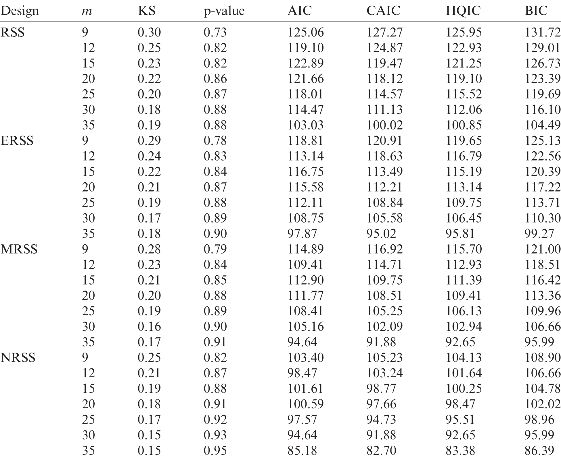
e. Conduct a GOF analysis and compare the empirical distribution for each replicate based on the likelihood estimators for all designs and compute the Kolmogorov–Smirnov (KS) statistic, Akaike information criterion (AIC), corrected Akaike information criterion (CAIC), Hannan–Quinn information criterion (HQIC) and Bayesian information criterion (BIC) for all fitted models. Compute an average KS statistic, AIC, CAIC, HQIC, and Schwarz-BIC indices.

The results of the simulation study are reported in Tabs. 1–4. The results for TRE, TRMSE, and p-values for KS test analysis are demonstrated in Figs. 2–4. From the results, the following comments are observed,

Table 1: Total relative efficiency and root total mean squared error for RSS-based estimators under perfect ranking and different designs

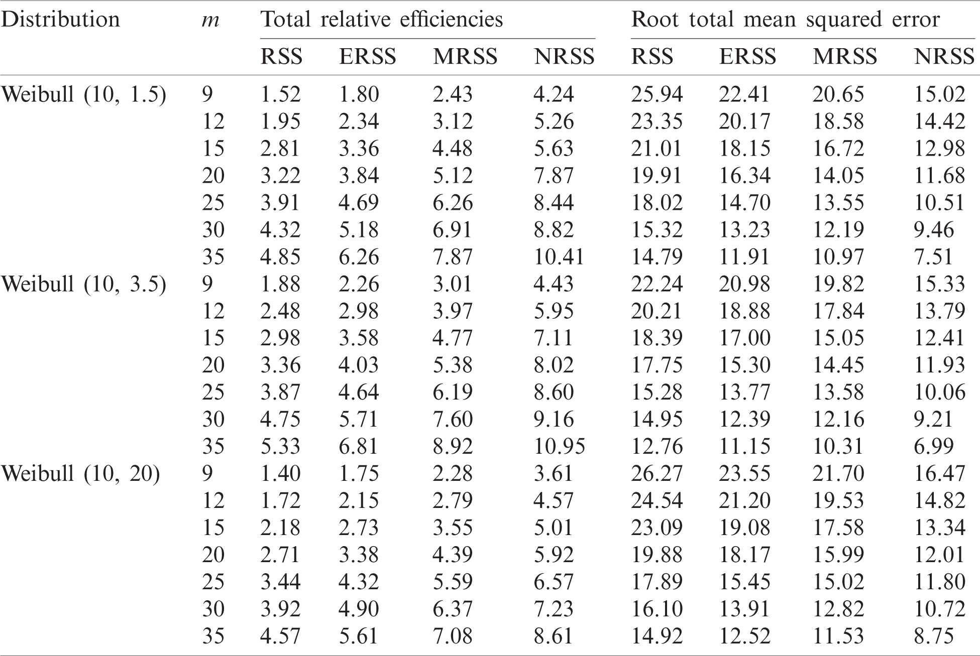
Table 2: GOF analysis for different sampling designs from Weibull (10, 1.5)

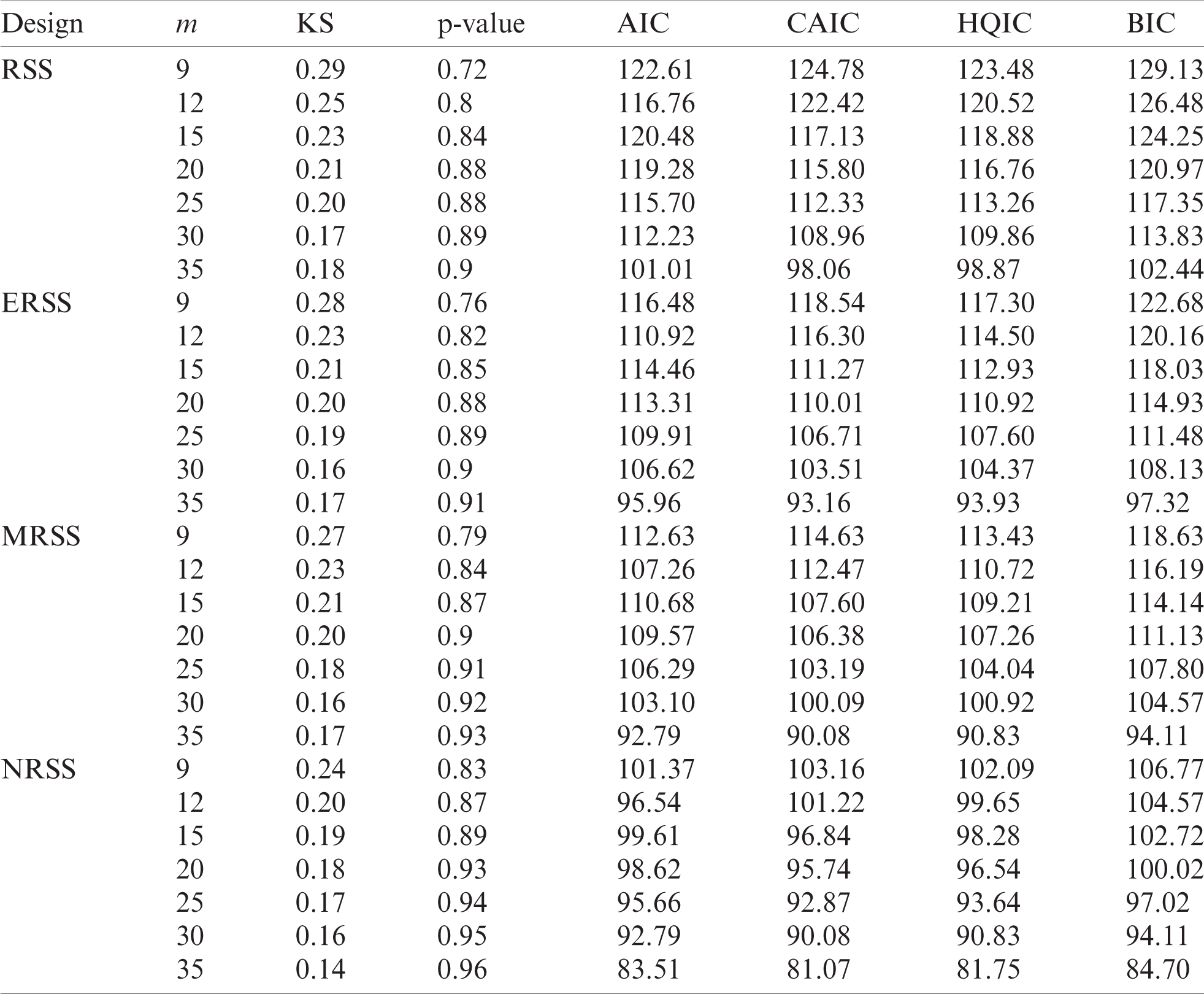
Table 3: GOF analysis for different sampling designs from Weibull (10, 3.5)

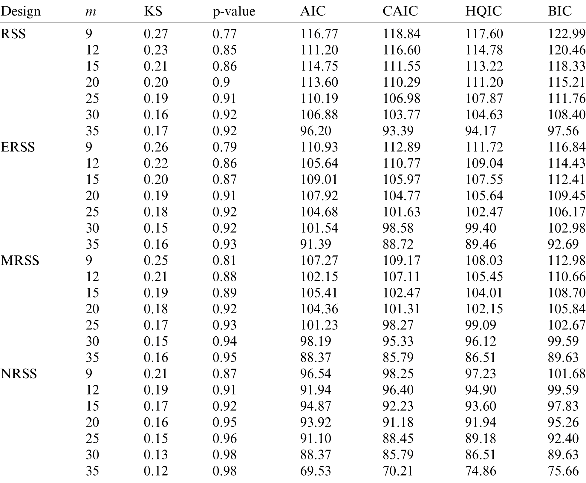
Table 4: GOF analysis for different sampling designs from Weibull (10, 20)

•   The total efficiency of all RSS-based designs increases as the sample size increases.

•   It is clear that the NRSS design provides the most efficient estimators and is superior to other sampling designs.

•   When the distribution shape is approximately symmetric, the RSS designs are more efficient than the corresponding efficiencies for asymmetric shapes.

•   Mean squared error decreases as the sample size increases and NRSS has the smallest MSE.

•   The GOF analysis showed that NRSS designs do have the highest p-value when testing the empirical distributions using KS test. Other GOF indices are the smallest for NRSS design relative to other RSS designs and they also decrease as the sample size increases.

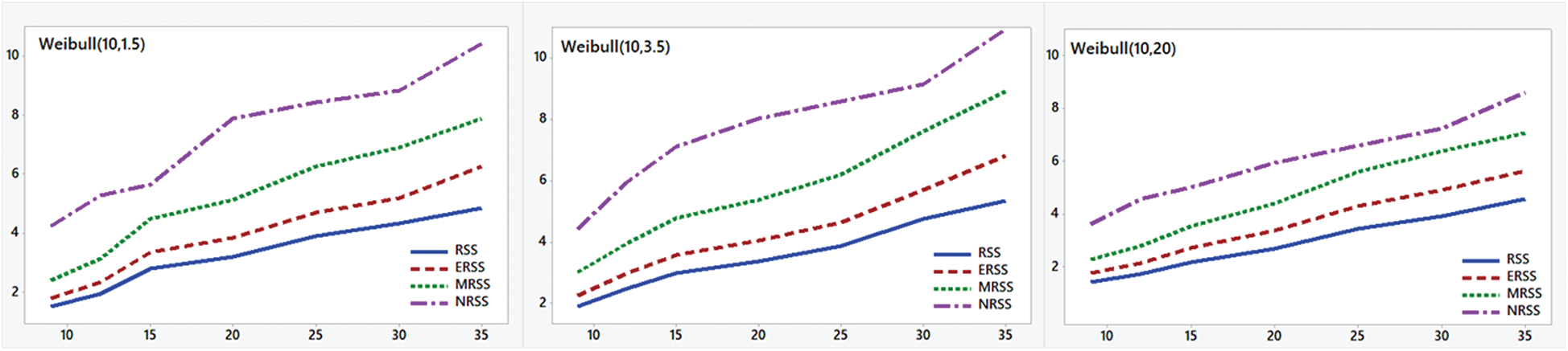
Figure 2: Total relative efficiency for different RSS sampling designs

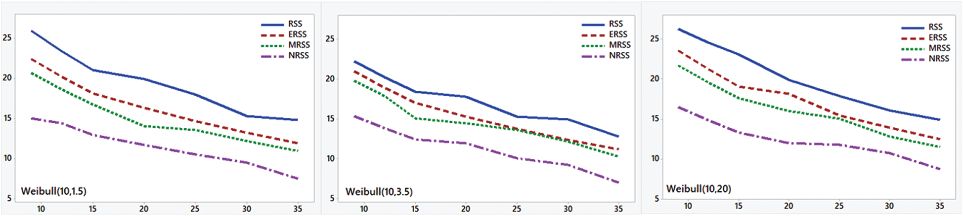
Figure 3: Total root mean squared error for different RSS sampling designs

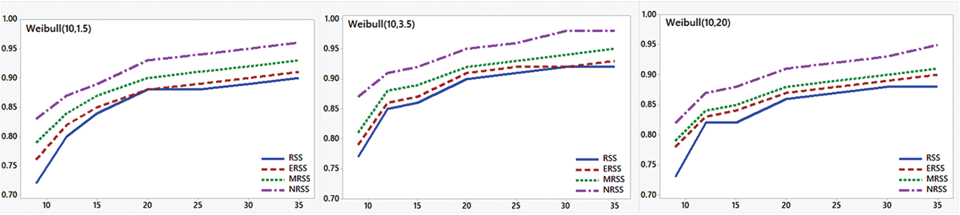
Figure 4: p-values for KS statistics for different RSS sampling designs

6  Conclusion

In this paper and based on numerical analysis, four RSS sampling designs were compared when estimating the parameters of the Weibull distribution. According to an extensive simulation study, it was possible to observe that under perfect ranking, the NRSS design outperforms the one-stage RSS, ERSS, and MRSS designs. Furthermore, it can be noted that the RTMSEs decrease as the set size increases, especially in asymmetric cases, and the total relative efficiency increases as the set size increases. Moreover, the NRSS design has the smallest MSEs and the largest efficiencies over the other sampling designs.

Acknowledgement: The authors are very grateful to the editor’s board and reviewers for their careful and fastidious perusing of the paper. The reviews are detailed and helpful to finalize the manuscript. The authors would like to kindly acknowledge them.

Funding Statement: The authors received no specific funding for this study.

Conflicts of Interest: The authors declare that they have no conflicts of interest to report regarding the present study.

References

 1.  G. A. McIntyre, “A method for unbiased selective sampling, using ranked sets,” Australian Journal of Agricultural Research, vol. 3, no. 4, pp. 385–390, 1952. [Google Scholar]

 2.  A. I. Al-Omari and K. Jaber, “Improvement in estimating the population mean in double extreme ranked set sampling,” International Mathematical Forum, vol. 5, no. 26, pp. 1265–1275, 2010. [Google Scholar]

 3.  H. M. Samawi, M. S. Ahmed and W. A. Abu-Dayyeh, “Estimating the population means using extremely ranked set sampling,” Biometrical Journal, vol. 38, no. 5, pp. 577–586, 1996. [Google Scholar]

 4.  H. A. Muttlak, “Median ranked set sampling,” J. Appl. Stat. Sci., vol. 6, no. 1, pp. 245–255, 1997. [Google Scholar]

 5.  M. T. Al-Odat and M. F. Al-Saleh, “A variation of ranked set sampling,” Journal of Applied Statistical Science, vol. 10, no. 2, pp. 137–146, 2001. [Google Scholar]

 6.  M. F. Al-Saleh and M. A. Al-Kadiri, “Double-ranked set sampling,” Statistics & Probability Letters, vol. 48, no. 2, pp. 205–212, 2000. [Google Scholar]

 7.  M. F. Al-Saleh and A. I. Al-Omari, “Multistage ranked set sampling,” Journal of Statistical Planning and Inference, vol. 102, no. 2, pp. 273–286, 2002. [Google Scholar]

 8.  E. Zamanzade and A. I. Al-Omari, “New ranked set sampling for estimating the population mean and variance,” Hacettepe Journal of Mathematics and Statistics, vol. 45, no. 6, pp. 1891–1905, 2016. [Google Scholar]

 9.  C. A. Taconeli and A. D. S. Cabral, “New two-stage sampling designs based on neoteric ranked set sampling,” Journal of Statistical Computation and Simulation, vol. 89, no. 2, pp. 232–248, 2019. [Google Scholar]

10. M. A. Sabry, H. Z. Muhammed, A. Nabih and M. Shaaban, “Parameter estimation for the power generalized Weibull distribution based on one-and two-stage ranked set sampling designs,” J. Stat. Appl. Prob., vol. 8, no. 2, pp. 113–128, 2019. [Google Scholar]

11. M. A. Sabry and M. Shaaban, “Dependent ranked set sampling designs for parametric estimation with applications,” Annals of Data Science, vol. 7, no. 2, pp. 357–371, 2020. [Google Scholar]

12. M. A. Stephens, “EDF statistics for goodness of fit and some comparisons,” Journal of the American Statistical Association, vol. 69, no. 347, pp. 730–737, 1974. [Google Scholar]

13. R. B. D’Agostino and M. A. Stephens, “Goodness-of-fit techniques,” in Basel(NYMarcel Dekker; Edited Version. Boca Raton, Florida, United States: CRC Press, 1986. [Google Scholar]

14. T. O. Yildiz and Y. C. Sevil, “Performances of some goodness-of-fit tests for sampling designs in ranked set sampling,” Journal of Statistical Computation and Simulation, vol. 88, no. 9, pp. 1702–1716, 2018. [Google Scholar]

15. W. Weibull, “A statistical distribution function of wide applicability,” Journal of Applied Mechanics, vol.18, no. 3, pp. 293–297, 1951. [Google Scholar]

16. D. A. Wolfe, “Ranked set sampling: An approach to more efficient data collection,” Statistical Science, vol. 19, no. 4, pp. 636–643, 2004. [Google Scholar]

17. D. V. Lindley, “Approximate bayesian methods,” Trabajos De Estadística y De Investigación Operativa, vol. 31, no. 1, pp. 223–245, 1980. [Google Scholar]

18. M. M. Nassar and F. H. Eissa, “Bayesian estimation for the exponentiated Weibull model,” Communications in Statistics-Theory and Methods, vol. 33, no. 10, pp. 2343–2362, 2005. [Google Scholar]

19. D. Kundu and B. Pradhan, “Bayesian inference and life testing plans for the generalized exponential distribution,” Science in China Series A: Mathematics, vol. 52, no. 6, pp. 1373–1388, 2009. [Google Scholar]

20. A. Xu and Y. Tang, “Reference analysis for Birnbaum–Saunders distribution,” Computational Statistics & Data Analysis, vol. 54, no. 1, pp. 185–192, 2010. [Google Scholar]

21. C. Kim, J. Jung and Y. Chung, “Bayesian estimation for the exponentiated Weibull model under Type-II progressive censoring,” Statistical Papers, vol. 52, no. 1, pp. 53–70, 2011. [Google Scholar]

22. R. Alshenawy, M. A. Sabry, E. M. Almetwally and H. M. Elomngy, “Product spacing of stress-strength under progressive hybrid censored for exponentiated-Gumbel distribution,” Computers, Materials & Continua, vol. 66, no. 3, pp. 2973–2995, 2021. [Google Scholar]

23. E. S. A. El-Sherpieny, E. M. Almetwally and H. Z. Muhammed, “Progressive type-II hybrid censored schemes based on maximum product spacing with application to power lomax distribution,” Physica A: Statistical Mechanics and its Applications, vol. 553, no. 1, pp. 124251, 2020. [Google Scholar]

24. R. Alshenawy, A. Al-Alwan, E. M. Almetwally, A. Z. Afify and H. M. Almongy, “Progressive type-II censoring schemes of extended odd Weibull exponential distribution with applications in medicine and engineering,” Mathematics, vol. 8, no. 10, pp. 1–19, 2020. [Google Scholar]

This work is licensed under a Creative Commons Attribution 4.0 International License, which permits unrestricted use, distribution, and reproduction in any medium, provided the original work is properly cited.