DOI:10.32604/cmc.2021.017461
| Computers, Materials & Continua DOI:10.32604/cmc.2021.017461 | |
| Article |
Optimal Sprint Length Determination for Agile-Based Software Development
1Department of Operational Research, University of Delhi, Delhi, 110007, India
2Department of Computer Science, Taibah University, Medina, 30001, Saudi Arabia
*Corresponding Author: Omar H. Alhazmi. Email: ohhazmi@taibahu.edu.sa
Received: 29 January 2021; Accepted: 22 March 2021
Abstract: A carefully planned software development process helps in maintaining the quality of the software. In today’s scenario the primitive software development models have been replaced by the Agile based models like SCRUM, KANBAN, LEAN, etc. Although, every framework has its own boon, the reason for widespread acceptance of the agile-based approach is its evolutionary nature that permits change in the path of software development. The development process occurs in iterative and incremental cycles called sprints. In SCRUM, which is one of the most widely used agile-based software development modeling framework; the sprint length is fixed throughout the process wherein; it is usually taken to be 1–4 weeks. But in practical application, the sprint length should be altered intuitively as per the requirement. To overcome this limitation, in this paper, a methodical work has been presented that determines the optimal sprint length based on two varied and yet connected attributes; the cost incurred and the work intensity required. The approach defines the number of tasks performed in each sprint along with the corresponding cost incurred in performing those tasks. Multi-attribute utility theory (MAUT), a multi-criterion decision making approach, has been utilized to find the required trade-off between two attributes under consideration. The proposed modeling framework has been validated using real life data set. With the use of the model, the optimal sprint for each sprint could be evaluated which was much shorter than the original length. Thus, the results obtained validate the proposal of a dynamic sprint length that can be determined before the start of each sprint. The structure would help in cost as well as time savings for a firm.
Keywords: Agile principles; agile-based software development; dynamic sprint length; multi-attribute utility theory; scrum; software development life cycle
Software is no longer restricted to sophisticated scientific activities, nor is it merely recreational or optional but a product of daily use. The Covid-19 pandemic forced the majority of the world into a lockdown. The changing times required us to practice social distancing and minimize physical human interactions. This forced us to adopt technology at a pace for which the world was not yet ready. To meet the gap, we need to come up with sustainable, adaptable, secure, and resilient software. We need to focus more on the quality of the product being created rather than the quantity. In the quest to reach the market early, quality should not be compromised. To ensure quality, one important point to be considered is the product creation process.
Software life cycle includes everything from its inception to its retirement. The software development life cycle (SDLC) is a systematic procedure for creating, deploying, and maintaining the software. Every piece of software undergoes a certain number of steps throughout its lifecycle: defining the requirements and their detailed analysis, designing the software, building the software, its rigorous testing and maintenance in the operational phase. The Waterfall Model, which was very widely used till a few years ago, lost its place due to its biggest drawback-rigidity. The waterfall approach does not allow scope for change in a particular phase once it is over. The Waterfall Model was designed to create small-scale projects, and it cannot meet the demands of complex systems required today. With changing times and demands, modified versions of the basic SDLC model appeared, and we now have a handful of SDLC models like the V-shaped model, spiral model, iterative and incremental model, agile-based models, prototype model, etc. These models follow the five steps of software development, but the order and implementation of each phase varies from model to model. Different software development projects use different SDLC models according to the project’s size, complexity, development cost, skill limitation, etc. These days, the most prevalent approach for software development is the Agile-based Software Development Life Cycle Model.
Before going into Agile Software development process details, one needs to understand the term agile and Agile Principles. The word agile means active and lively, and represents something quick and well-coordinated. It is a mindset that helps to deal with uncertainty. Keeping this in mind, the Agile Manifesto was designed in 2001 by 17 people who laid the ground rules of a new technique [1].
The Agile Manifesto gave higher importance to customer satisfaction, active user involvement, simplicity, welcoming change, working on software, face-to-face conversations, frequent and continuous delivery, working together daily, reflections, and adjustment, among other things. The manifesto did not provide a methodology or a method. Instead, it provided the principles which could make a methodology agile. The Agile Principles can be applied to software development, project management, business management, etc., and are being used in the construction industry, education sector, marketing and advertising companies, finance-related industries, and event planning, to name a few.
The agile software development process follows an incremental and iterative approach. The whole project is divided into small incremental builds where each iteration (sprint) adds specific functionality to the previous build. At the end of each sprint, we obtain a working product, which is presented to the user. The user is highly involved in the development process, and their feedback is incorporated in the next iteration. The process is perceived to be very lightweight because of the low amount of documentation work required. The Agile SDLC can overcome the waterfall model’s major shortcomings by being highly flexible, fast, and responsive.
Like any other technique, Agile SDLC also has a fair number of shortcomings. It requires a team of highly skilled professionals who can handle the dynamic development environment. The user also needs to be very clear about the product they want. Without these, the project can easily overrun the budget, the time, and often result in an unsatisfied customer.
There are numerous agile-based approaches available but among these, the Scrum development process is widely used for software development. According to the State of Agile Report [2], 75% of the 40,000 surveyed agile executives used Scrum or a modified version of it. Scrum is a framework for developing and sustaining complex projects. In 2013, Sutherland et al. [3] wrote the Scrum Guide, which is an industry-standard document defining the Scrum process and its implementation. According to them, “Scrum is a framework within which people can address complex adaptive problems, while productively and creatively delivering products of the highest possible value. Scrum is lightweight, simple to understand and difficult to master.” The word Scrum was picked up from the word scrummage, a rugby formation, to denote the high-performing, cross-functional teams in the scrum process. Scrum has been used to develop software, hardware, embedded software, networks of interacting function, autonomous vehicles, schools, government, marketing, managing the operation of organizations and almost everything we use in our daily lives, as individuals and societies.
The Scrum defines three groups: product owner, scrum master, and the development team. The members of the development team create the Increment, i.e., a workable functionality. The Increment may be a small part of the whole product, but it is standalone complete. In the initial sprints, priority is given to those functionalities which are the essence of the product. Here, the 80–20 rule is followed, i.e., 80% of the functionality is contained in 20% of the code and only the most essential features are developed.
The progress in the Scrum framework can be understood through Fig. 1. Each development project has a comprehensive list of requirements called the product backlog. It is a dynamically changing document wherein the requirements of feature enhancements, functions, features, etc. keep changing as the product progresses. The tasks mentioned in the product backlog are arranged in the order of their priority and an achievable target is set for each Sprint. This sprint planning is done through collaboration of the whole scrum team. The sprint backlog is a subset of the product backlog to be catered to in a particular sprint. Sprint backlog plans the delivery of the sprint and the plan to achieve it. It is a highly visible, real-time picture of the work that the development team plans to accomplish during the sprint, and it belongs solely to the development team.
Sprints contain the sprint planning, daily scrums, the development work, the sprint review, and the sprint retrospective. Each sprint has a defined task and a flexible plan to achieve it. The Scrum requires the sprint length to be fixed, but it usually varies at the start of the project when the right fit is being determined. For a shorter duration project, the sprint length is kept shorter, while for a longer duration project, it is kept around four weeks. As per Scrum guidelines, a sprint must not be shorter than one week or exceed four weeks. It is this attribute around which this present proposal revolves. Here, an attempt has been made to understand the reasons for the above time limits and show that these cannot always be followed under every condition. The sprint duration would depend on the situation.
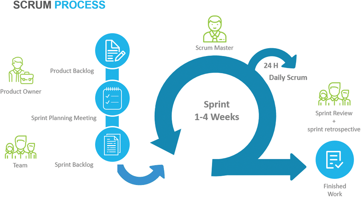
Figure 1: The scrum framework
The current proposal has been designed as follows. Section 2 discusses the literature review and the research questions addressed in the current proposal. The notations used in the model development have been discussed in Section 3, followed by the detailed mathematical framework in Section 4. To show the applicability of the developed model, an illustration has been discussed in Section 5. Section 6 concludes the work and is followed by a list of references to the articles used in this work.
In the recent past, the use of Agile practices in software development has attracted the attention of developers and researchers. Reference [4] compared and analyzed the various Agile-based software development techniques. Reference [5] have provided a detailed literature review on the use of Scrum in software development. Reference [6] explored the Agile practices through the Agile wheel reference model (AWRM). Reference [7] identified the challenges in adopting Agile. Reference [8] wrote comprehensive literature on the principles, evolution and criticisms of the Agile development approach. Reference [9] explored the importance of the various principles of Agile methods and their relationships. Reference [10] discussed the implementation of Agile practices in maintenance activities. Reference [11] evaluated the teamwork quality and its impact on the success of an agile-based software development project. Reference [12] identified the important factors which are necessary for successful implementation of lean Six-sigma implementation. Reference [13] combined the best practice of open-source software development (OSSD) and Scrum to create OSCRUM. Reference [14] proposed the S-SDLC model, which uses Agile principles to maximize software security without compromising its quality. Reference [15] identified the shortcomings of Scrum and how it has evolved into Scrumban. They also proposed a new framework, Structured Kanban Iteration (SKI), for DevOps and continuous delivery.
The Agile technique has been very well explained theoretically, but few mathematical models exist to explain its dynamics. Reference [16] proposed a linear optimization model to plan the multiple sprints. Reference [17] conducted an empirical study on the distribution of software metrics in software developed using Agile principles. Reference [18] proposed quantitative measures to assess the quality and reliability of software developed using Agile methods. Reference [19] have discussed using non-homogenous Poisson process (NHPP) based models to determine the reliability of software in an Agile-based environment. Reference [20] discussed a mathematical framework for the fault removal process in the multiple sprints of Agile software.
It can be observed from the set of aforesaid studies that though much work has been done in the context of Agile development, only a small number of researchers have discussed the optimal sprint length and its determination. The research in the current work has attempted to further improve the Agile method, specifically Scrum, by using mathematical models. The aim and scope of this research have been discussed through the following research questions.
Research Question 1: Do we really need a fixed Sprint Length?
The Scrum guidelines [3] require a fixed sprint length throughout the project. The factors taken into consideration are the project duration, the environment provided by the customer or the stakeholders in the project, the work efficiency of the Scrum team, etc. Whatever the optimal length is determined to be, it is considered the same for each sprint. A very valid question that arises here is why is it necessary to have a predetermined sprint length for each sprint? And can different sprints have different sprint lengths?
The manifesto developers chose the word agile because it represented adaptiveness in response to change, which was important for the process they were defining. Even though the Scrum development process effectively implements the Agile principles, it still maintains rigidity in the sprint length determination. Nevertheless, in practice, not each sprint requires the same number of days. While some tasks may take a longer time, others may not need the predetermined one week or so. On implementation, it was found that not all user stories can be defined so that they meet the definition of done (DOD) in a single sprint. Often extra days or extended working hours were required, i.e., a buffer period or a buffered sprint was needed to complete a given task. In Scrum, a sprint is a time-boxed event, and tasks are broken down in such a way that they fit into these time frames. However, it seems that we require an alternative approach which is task-bound and the sprint length is determined considering the task. The wasted time, effort, and resources spent waiting for the next sprint to begin or the need to lengthen a sprint should be catered to in the planning process. The agile process is about adaptability and flexibility. We propose that this flexibility should be extended to the sprint, and the duration of each sprint should be dynamic.
Research Question 2: What are the possible benefits or repercussions of varying the Sprint Length?
After an extensive search, we concluded that no notable research work has been done regarding sprint length. Hence, we had to rely heavily on the experiences shared on various discussion forums and blogs to support our claim. The opinions of people and their problems with sprint length implementation expressed on the Internet fall into two major classes. The first is those who strictly follow the Scrum guidelines and hence opine that sprints should be time-boxed events that cannot be changed. Further, the current sprint length should never be altered to consider the leftover tasks of a sprint that might require a day or two more to reach a deliverable. Many arguments for the same can be found on Quora and Reddit, which are mostly centered on consistency. A repeatedly changing sprint length brings uncertainty into the work environment. For a big firm, where a resource person is simultaneously working on several projects, different sprint lengths in different projects can be confusing. Another major concern that arises is measuring the velocity of the team in an ever-changing scenario [21].
Another option is the implementation of a buffer sprint, which allows an extra day or so to complete the sprint goal. The buffer also allows the developers to deal with unexpected tasks that crop up amid a sprint and take precedence over the other tasks. Different firms use different strategies: Some earmark a fixed percentage of their time and resources as a buffer, while others may vary it or deal with it as and when the situation arises. Reference [22] conducted a study to see what changes a company makes while implementing Scrum. According to their conclusion, one of the surveyed companies allowed flexibility in the sprint length for developing a new product but not in the cases of enhancing established products. Most companies did not calculate a buffer in the sprint task but some used a variable or fixed buffer time for various needs like unforeseen works, technological issues, debugging, etc. The work of [15] discussed the issues faced in implementing Scrum and the issue of a fixed sprint length. They also suggest that a fixed sprint length does not always make sense; it can be varied according to the project need. Furthermore, aiming to break down each requirement to fit in a fixed time frame may not always be possible.
One apparent reason for this conflict of opinions is that one size cannot fit all. Not all firms can implement Scrum according to the guidelines. The nature of the project, the work environment, the team members, etc. all influence the sprint outcome.
Dynamic sprint length can be implemented by deciding the sprint length in the sprint planning phase, keeping in mind the sprint goals. Since the sprint length will be determined at the start of the iteration itself, there should not be any confusion about the next sprint’s start time. A dynamic sprint length would allow better utilization of the time, manpower, and other project resources. The optimal time allocation for certain tedious tasks would reduce the developers’ deadline stress and eventually lead to greater productivity. According to [23], there is a U-shaped relationship between time pressure and productivity, i.e., too much time pressure from the boss can decrease the employees’ output and cause higher user stories being carried over to the next sprint which, in turn, will increase the technical debt. The unexpected bugs and discrepancies can also be easily tracked and tackled. Often, when new teams implement Scrum, there is a remarkable increase in their output. The tasks which were likely to be completed over several sprints are completed in a single sprint. In such cases, when the team has more time than required, productivity can often decrease. Factors such as procrastination, lack of motivation, and the effect demonstrated by Parkinson’s Law [24] come into play. Thus, the tasks which could have been completed earlier take much longer. This has immediate economic repercussions and impacts on the team’s spirit, individual morale, and long-term output.
Research Question 3: How to determine the Optimal Sprint Length for a particular sprint?
Organizations new to the Agile development process commonly follow the practice of altering the sprint length till the best fit is found. Moreover, these organizations find the solution either intuitively or by trial and error as they seek the best fit. A decision-making approach that considers different attributes and finds the trade-off for the various attributes mathematically could prove more efficient and less effortful, and cost-and time-effective. The current proposal presents a mathematical model that considers the number of enhancements/tasks to be dealt with in a sprint and the cost incurred in its implementation. We have used MAUT, a multi-criterion decision making (MCDM) technique to determine the optimal sprint length.
The notations used in the development of the model are as follows:
n: The total number of sprints required to complete the project.
i: A counter variable representing a particular sprint,
ai: Number of tasks in the ith Sprint of software
ci0: Per unit developmental cost for ith Sprint
ci1: Developmental cost for the user stories in ith Sprint’s backlog
ci2: Developmental cost for the leftover stories of
ci3: Cost incurred in performing additional tasks in the ith Sprint
cB: Total developmental budget available for the project
In the current modeling framework, the focus is on determining the suitable sprint length. As discussed earlier, the development team actively works and manages its activities to achieve the sprint goal. The teams often have to deal with some tasks that could not be completed in the previous sprint and have to be dealt with now. Moreover, a sprint may include various tasks such as bug repair, feature enhancement, and new feature development. The development team’s job is to incorporate all these tasks and write reliable code. The reliability of the code is tested rigorously.
The optimal sprint length is determined as follows. In the first section, Section 4.1, we have determined the number of tasks that will be dealt with in a particular sprint. Section 4.2 discusses the costs which would be incurred in completing these tasks. Section 4.3 uses the optimization tool MAUT to determine the optimal sprint length with the help of the framework obtained from Sections 4.1 and 4.2.
4.1 Modeling the Software Developmental Process
This section discusses the modeling framework for the software development process through various sprints. Each of the tasks to be performed in the sprint is assigned to one of three categories, namely, the items in the sprint backlog of the particular sprint, the leftover items from the previous sprint (Technical debt) that should be catered to in the current sprint, and the issues which may arise when the increment of the previous sprint becomes operational. The third category would also include the changes necessary in the product after the stakeholders and customers/users give their feedback on the product. These tasks could be refactoring and debugging. The tasks of this category may or may not arise. Depending on the project and the stakeholders, these changes might be demanded in the ongoing sprint or may be deferred to the next sprint. According to [25], 54% of the high-level requirements are not met in their planned iteration. The rising technical debt compels the developers to pass on tasks to the next iteration.
The modeling framework bears a close resemblance to the fault removal phenomena in software reliability. Hence, we have drawn an analogy from the software reliability literature and defined an NHPP-based model that defines the expected number of tasks dealt with till a given time t. It can be mathematically represented using the approach discussed in [19,26] as:
where k(t) represents the expected number of tasks performed in a sprint till time t; A represents the initial number of tasks which were to be performed throughout the Sprint; Z(t) is the probability distribution function and Z(t) is the cumulative distribution function which defines the pattern in which tasks are performed. Also,
Here, we can define
On solving Eq. (2) with initial condition, i.e., at
Here, Z(t) can take different functional forms depending on the nature of the data, problem etc.
For a better visual understanding, a timeline has been shown in the following Fig. 2.
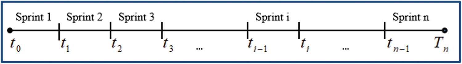
Figure 2: Timeline depicting the subsequent sprints
Using the generalized structure for k(t) in Eq. (3), the phenomena for the different sprints can be described as follows.
4.1.1 Modeling Pertaining to Sprint 1
Sprint 1 is the first iteration, and it occurs between time (t0, t1). All the sprint activities, such as sprint planning, daily scrum, designing, development, and testing occur here. The teams set out with a predefined set of tasks outlined in the sprint backlog. The expected number of tasks that will be completed in the first sprint can be mathematically expressed as:
where A
4.1.2 Modeling Pertaining to Sprint 2
The second sprint (t1, t2) adds on to the software created in the first sprint. Each phase of the SDLC is revisited and with the mutual understanding and joint efforts of the various teams, features are added in the second sprint. Software testing is carried out and any leftover tasks of the previous sprint along with the new features, if any, requested by the user are incorporated here. Any tasks which could not be completed in the first sprint will also be completed here. It can be represented as:
where A
4.1.3 Modeling Pertaining to Sprint 3
The third sprint (t2, t3) is the third iteration in the development cycle which means the product has begun taking a fairly good shape and evolving toward the desired end product. Feature enhancements are made by developing the user stories in the sprint backlog. The following Eq. (6) models the said phenomena as:
where A
4.1.4 Modeling Pertaining to ith Sprint.
The ith sprint (ti −1, ti) represents any general sprint. As discussed earlier, any sprint will be dealing with three major categories of tasks. The modeling framework for the ith sprint (ti −1, ti) can be represented as follows:
where
Using the mathematical structure described here, the cost modeling has been computed in the following section.
4.2 Cost Modeling for the Sprints
Each project starts with a fixed budget which is allocated to the various processes. Four types of costs that will be incurred in the developmental process are identified here. The per-unit development cost majorly meets the cost incurred whether or not any progress is made, i.e., the cost incurred till the time the team is working on the current project. It could also include all the indirect costs incurred on tasks that help improve the team’s output. The second cost is the cost of developing a new user story. It will consume a major portion of the budget. The third cost is the cost incurred on completing the leftover stories of the previous sprint. It will also include the penalty for not meeting the deadline and loss of opportunity. The fourth is the cost that will be incurred on performing additional tasks. It could include the changes that the customer has suggested after reviewing the increment of the previous version, some debugging activity, or some security issue, etc., which will take precedence over the designated sprint tasks. This cost needs to be defined separately because it is much easier to write an altogether new code than re-visit an old code and debug it.
Here, we have represented the cost structure for the first three sprints, followed by a generalized representation for the ith sprint.
4.2.1 Cost Structure for Sprint 1
The cost incurred in the first sprint of the software
4.2.2 Cost Structure for Sprint 2
The cost incurred in Sprint 2 C
4.2.3 Cost Structure for Sprint 3
The total cost for Sprint 3 can be represented as:
The cost incurred in the Sprint C
4.2.4 Cost Structure for ith Sprint
The cost associated with the ith sprint Citotal will comprise the following four costs: developmental cost throughout the sprint, i.e., Ci0t; the cost of developing new user stories in the sprint, i.e.,
and c12 = 0 for the first sprint.
4.3 Optimal Sprint Length Determination
Software engineers not only want the system to be secure, but they also wish to minimize the money, time, and resources spent on the project. There are several existing techniques, algorithms, and theories on how to make a better or the best decision in a given situation. Multi-attribute utility theory (MAUT), one such decision-making technique, relies heavily on the utility theory from the field of economics to quantify the preference or the satisfaction derived from a particular attribute. MAUT provides a trade-off between the desired values of multiple conflicting attributes. Each attribute has its set of constraints and the decision-maker decides how much they are willing to give up or derive from an attribute.
Major contributions to the field were made by [27–29]. Reference [30] used MAUT in the context of product remanufacturing. In the field of software reliability, [31–33] have used MAUT to determine software release time in various situations. The present proposal has used their work as a guideline.
Methodology for developing the utility function for MAUT follows a four-step decision-making process:
• Selection of attributes
We were able to identify the scope of the sprint and investment as the most important attribute. For computational purposes, we have interpreted the scope of the sprint as the number of tasks that have to be performed in a sprint. The team’s performance can be measured by the number of tasks performed and the effort required to maximize that number with each successive sprint, i.e., maximize the team’s work intensity. It is highly desirable, especially in agile-based processes, to maximize the team’s output and achieve the team’s maximum potential. If the work intensity is low, the teams will most likely not achieve the sprint goal and will produce compromised software in terms of quality and security [34].
Given k(t), we can define the objective function for work intensity,
The second attribute is the cost incurred in performing the number of tasks in a sprint which we wish to minimize. If the project cost overruns, it can lead to a financial loss for the firm, opportunity loss, and bad word-of-mouth publicity. If an affordable product is developed, the cost to the end-user would also be modest and it will attract a larger number of buyers. Hence, the objective for the ith sprint under MAUT is:
• Selection of attribute bounds
The decision-maker should choose the bounds of the attributes. The best and the worst performance in an individual attribute is denoted by the upper and lower bounds, respectively. All the possible outcomes for an attribute lie between these bounds. The best and worst values of work intensity are denoted by
• Estimation of weight parameters
The weights associated with work intensity and budget have been taken as
• Structure of MAUF (Multi-Attribute Utility Function)
Based on the Single-Attribute Utility Function (SAUF), the scaling constants for each attribute in the MAUF in additive linear form can be given as:
where
SAUF of the work intensity and cost are
where
The proposed model can be validated on any dataset that contains a detailed description of the project development process. The project requirements can be broken down into epics and user stories to create the product backlog. Project planning would lead to prioritizing these tasks and planning the sprints, sprint goal, and sprint backlog. The initial values of the parameters thus obtained can be used to evaluate the model using the non-linear least square method. The lack of access to such privy details of any project forces us to perform our model validation on secondary data.
For this, let us consider a special case wherein the set of activities in a sprint is related to the debugging process of, for example, a project on software maintenance. The dataset given by [20], which contains a description of 287 faults that were debugged in 7 sprints, has been used in this study. The length of each sprint was fixed at four weeks. The structure of the problem defined in section 4 remains the same. The interpretation changes slightly as the ai now corresponds to the task of debugging in the ith sprint. The previous sprint’s leftover tasks now refer to the faults that could not be perfectly removed in the earlier sprint and must be dealt with in the next one. The current project does not consider additional tasks hence,
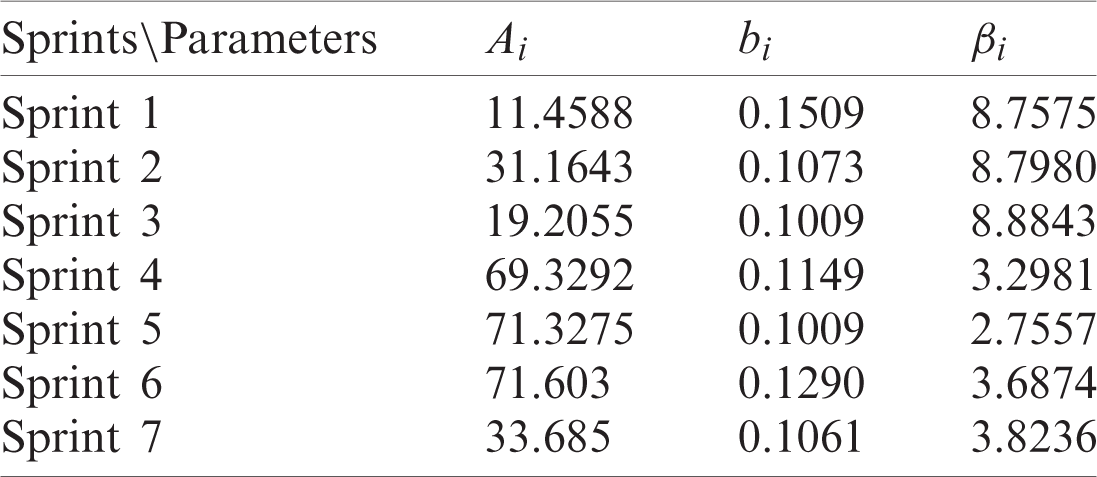
Considering the nature of the data used here, we have assumed that the rate of performing the tasks is logistical [26]. Hence, taking
The Statistical Analytical Systems (SAS) software [35] was used to estimate the parameter values of the equations set out in Section 4.1 and the values obtained for each sprint are shown in the following Tab. 1.
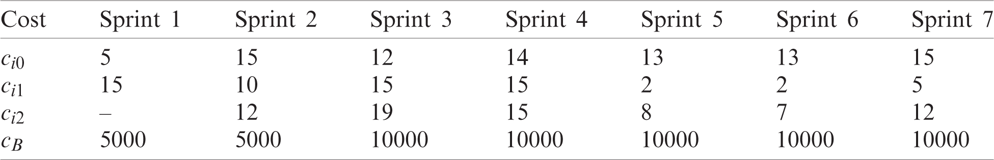
Tab. 2 shows the assumed cost parameters used to evaluate each sprint’s total cost as discussed in Section 4.2.
Table 2: Assumed values for Cost Parameters (1
Using the estimated values of the parameters (Tab. 1) and assumed values of cost (Tab. 2), we have evaluated the optimization problem (Eq. 15) defined in Section 4.3.
For our example, we have taken the least value of the work intensity (which is failure intensity) to be 60% and maximum to be 100%. For the cost attribute, we want the least consumption to be 70% and the maximum consumption to be 100%. Further, we have assigned equal weight to both the attributes, i.e., 0.5.
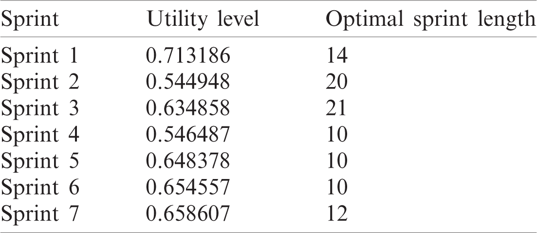
Tab. 3 shows the optimal sprint length and the utility value achieved by taking both the cost and work intensity as attributes.
Table 3: Utility values and optimal sprint length
The utility curves obtained after the application of MAUT are as shown in Figs. 3–9.
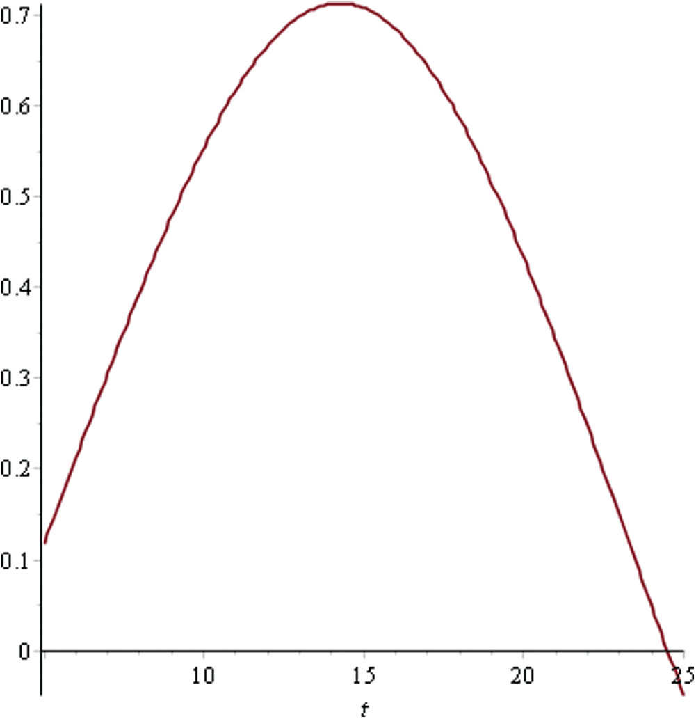
Figure 3: Utility curve for sprint 1
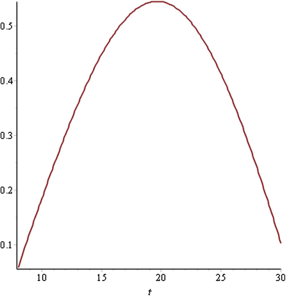
Figure 4: Utility curve for sprint 2
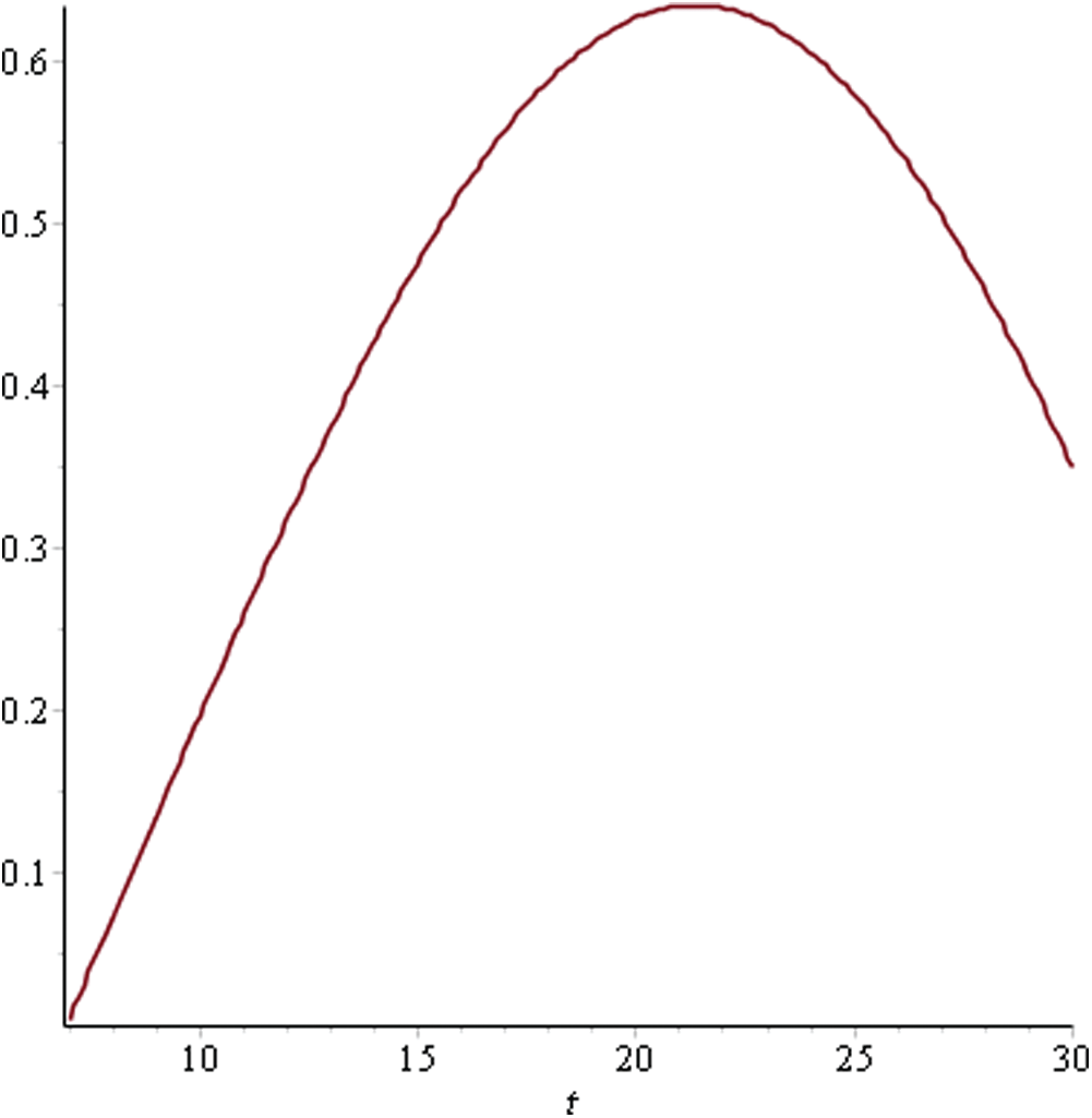
Figure 5: Utility curve for sprint 3
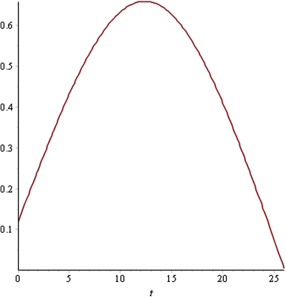
Figure 6: Utility curve for sprint 4
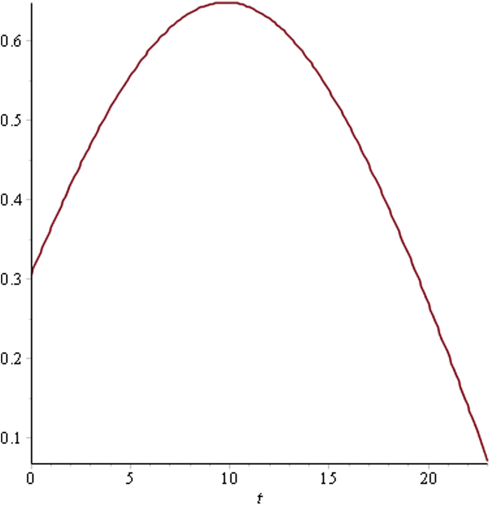
Figure 7: Utility curve for sprint 5
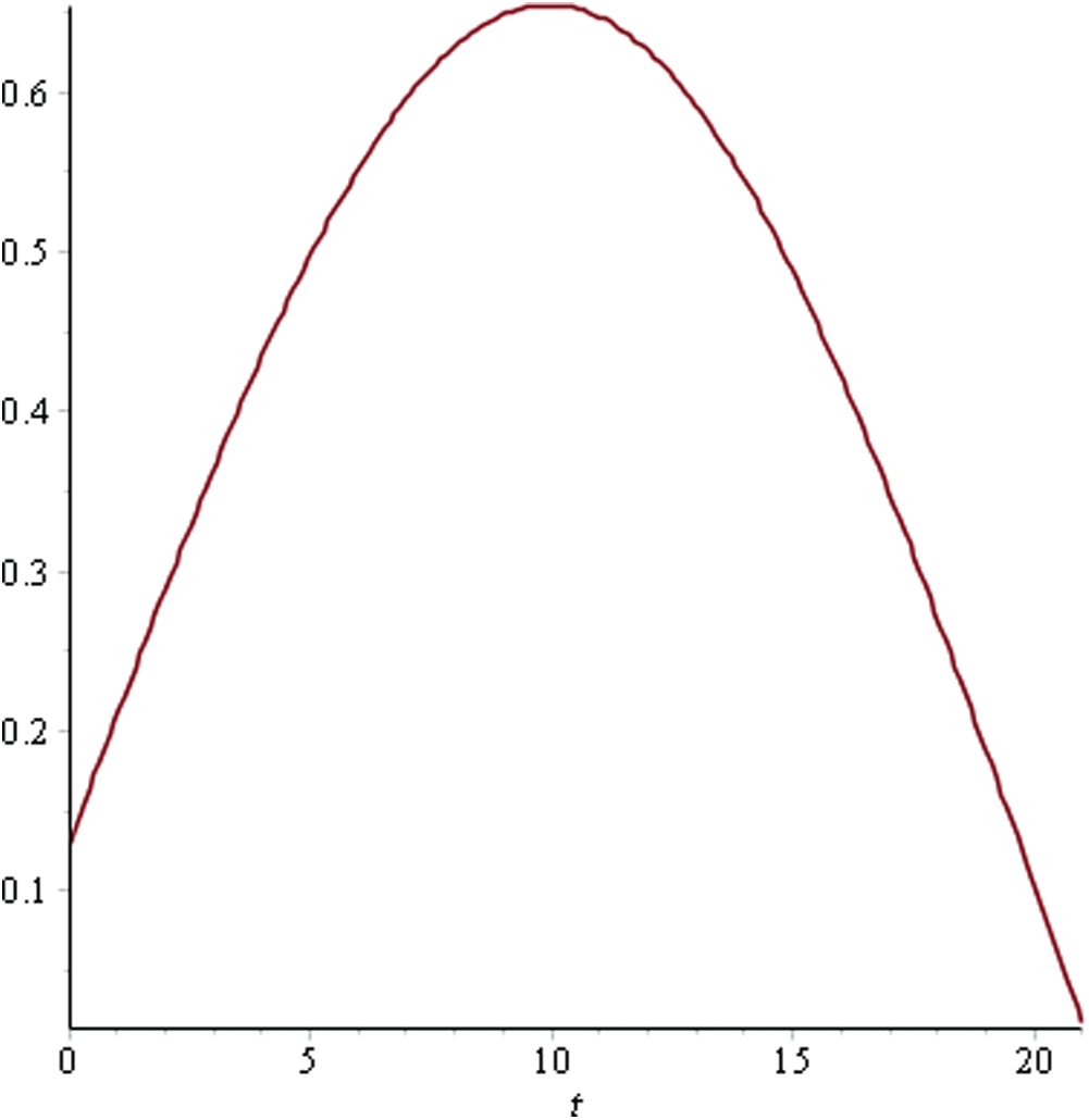
Figure 8: Utility curve for sprint 6

Figure 9: Utility curve for sprint 7
As can be seen in Fig. 4, the maximum utility that can be achieved is 0.71 for Sprint 1 at time point 14. This indicates that having a sprint length greater than this would lead to a reduced utility level due to the attributes. In Sprint 2, the utility curve reached its maximum value of 0.54 at the 20th time point. Hence, the ideal sprint length in such a situation would be 20 days. Similarly, in Sprint 3, the maximum utility that could be achieved was 0.63 at time point 21. For Sprints 4–6, the utility curve attained its peak at the 10th time point with a maximum utility level of 0.54, 0.64, and 0.65, respectively. Hence, the ideal sprint length for these three sprints should be 10 days instead of the originally considered 30 days. In Sprint 7, the maximum utility level of 0.65 was attained at the 12th time point.
The results show especially clearly when the two attributes, work intensity (failure intensity) and cost, are considered simultaneously. Then the optimal sprint length is around or less than 20 days. According to the current cycle, 30 days are being spent on a single sprint. Thus, for the resources to be used optimally, the sprint length cannot be fixed. It would be better to mathematically determine the length of each sprint beforehand based on the tasks to be handled in each sprint and the availability of resources. An alternative to the commonly used fixed sprint length approach is proposed here. It provides a mathematical basis to treat a sprint as a task-based event instead of a time-bound event.
Currently, Agile-based models are the most prevalent technology for software development. Scrum, an Agile-based model, develops the software through successive iterations known as sprints. The sprint length is generally taken to be 1–4 weeks and is predetermined by the firm. The main aim is to complete every task in the sprint within the allotted time. If the sprint needs more time to complete, the leftover tasks are deferred to the next sprint. Often, the tasks allocated for a sprint take up less or more time than the fixed sprint length. Therefore, it is proposed that the sprint length should be based on the tasks to be performed in it. The length could be different from sprint to sprint. This would help to do away with the uncertainties caused by buffer sprints. It is further proposed that the length be determined mathematically before undertaking each sprint instead of being fixed at the beginning of the project. A mathematical framework has been discussed here to determine the optimal sprint length for each sprint within the available budget and at the required work intensity. The results obtained here satisfactorily support the claimed advantage of having dynamic sprint length. According to the case discussed here, the determined sprint lengths were much shorter than the fixed lengths and there was considerable time-saving in each sprint. In future work, if the appropriate data is available, the application of the proposed method can be fully demonstrated. It is also proposed to explore how the dynamic sprint length can be determined in a distributed environment.
Funding Statement: The authors received no specific funding for this study.
Conflicts of Interest: The authors declare that they have no conflicts of interest to report regarding the present study.
1. K. Beck, M. Beedle, A. Van Bennekum, A. Cockburn, W. Cunningham et al., “Manifesto for agile software development,” 2001. [Online]. Available: https://agilemanifesto.org/. [Google Scholar]
2. VersionOne Inc., “The 14th annual state of agile report,” Technical Report, VersionOne Inc., 2020. [Online]. Available: https://stateofagile.com/. [Google Scholar]
3. J. Sutherland and K. Schwaber, The Scrum guide. In: The Definitive Guide to Scrum: The Rules of the Game, pp. 268, 2013. [Online]. Available: SCRUM.org. [Google Scholar]
4. P. Abrahamsson, O. Salo, J. Ronkainen and J. Warsta, Agile Software Development Methods: Review and Analysis, vol. 478. Espoo, Finland: VTT publication, pp. 107, 2002. [Google Scholar]
5. E. Hossain, M. A. Babar and H. Y. Paik, “Using scrum in global software development: A systematic literature review,” in Proc. Fourth IEEE Int. Conf. on Global Software Engineering, Limerick, Ireland: IEEE, pp. 175–184, 2009. [Google Scholar]
6. S. Meredith and D. Francis, “Journey towards agility: The agile wheel explored,” TQM Magazine, vol. 12, no. 2, pp. 137–143, 2000. [Google Scholar]
7. S. C. Misra, V. Kumar and U. Kumar, “Identifying some critical changes required in adopting Agile practices in traditional software development projects,” International Journal of Quality & Reliability Management, vol. 24, no. 4, pp. 451–474, 2010. [Google Scholar]
8. S. Misra, V. Kumar, U. Kumar, K. Fantazy and M. Akhter, “Agile software development practices: Evolution, principles, and criticisms,” International Journal of Quality & Reliability Management, vol. 29, no. 9, pp. 972–980, 2012. [Google Scholar]
9. M. Doyle, L. Williams, M. Cohn and V. Rubin, “Agile Software Development in practice,” in G. Cantone, M. Marchesi (EdsAgile Processes in Software Engineering and Extreme Programming. XP 2014. Lecture Notes in Business Information Processing, vol. 179. Cham, Switzerland: Springer, 2014. [Google Scholar]
10. L. T. Heeager and J. Rose, “Optimising Agile development practices for the maintenance operation: Nine heuristics,” Empirical Software Engineering, vol. 20, no. 6, pp. 1762–1784, 2015. [Google Scholar]
11. Y. Lindsjørn, D. I. Sjøberg, T. Dingsøyr, G. R. Bergersen and T. Dybå, “Teamwork quality and project success in software development: A survey of agile development teams,” Journal of Systems and Software, vol. 122, no. 3, pp. 274–286, 2016. [Google Scholar]
12. L. Papic, M. Mladjenovic, A. Carrión García and D. Aggrawal, “Significant factors of the successful lean six-sigma implementation,” International Journal of Mathematical, Engineering and Management Sciences, vol. 2, no. 2, pp. 85–109, 2017. [Google Scholar]
13. S. S. M. M. Rahman, S. A. Mollah, S. Anirban, M. H. Rahman, M. Rahman et al., “OSCRUM: A modified scrum for open-source software development,” International Journal of Simulation: Systems, Science and Technology, vol. 19, no. 3, pp. 20–21, 2018. [Google Scholar]
14. J. De Vicente Mohino, J. Bermejo Higuera, J. R. Bermejo Higuera and J. A. Sicilia Montalvo, “The application of a new secure software development life cycle (S-SDLC) with Agile methodologies,” Electronics, vol. 8, no. 11, pp. 1218, 2019. [Google Scholar]
15. J. Saltz and A. Sutherland, “SKI: A new agile framework that supports, develops, continuous delivery, and lean hypothesis testing,” in Proc. of the 53rd Hawaii Int. Conf. on System Sciences, Hawaii, United States, pp. 6217–6226, 2020. [Google Scholar]
16. M. Golfarelli, S. Rizzi and E. Turricchia, “Multi-sprint planning and smooth replanning,” An optimization mode Journal of Systems and Software, vol. 86, no. 9, pp. 2357–2370, 2013. [Google Scholar]
17. G. Destefanis, S. Counsell, G. Concas and R. Tonelli, “Software metrics in Agile software: An empirical study,” in Proc. Int. Conf. on Agile Software Development, Rome, Italy: Springer, Cham, pp. 157–170, 2014. [Google Scholar]
18. S. Yamada and R. Kii, “Software quality analysis for Agile development,” in Proc. 4th Int. Conf. on Reliability, Infocom Technologies and Optimization (Trends and Future DirectionsAmity University Uttar Pradesh (AUUPNoida, India: IEEE, pp. 1–5, 2015. [Google Scholar]
19. S. Rawat, N. Goyal and M. Ram, “Software reliability growth modeling for agile software development,” International Journal of Applied Mathematics and Computer Science, vol. 27, no. 4, pp. 777–783, 2017. [Google Scholar]
20. P. Mishra, A. K. Shrivastava, P. K. Kapur and S. K. Khatri, “Modeling fault detection phenomenon in multiple sprints for Agile software environment,” in Quality, IT and Business Operations. Singapore: Springer, pp. 251–263, 2018. [Google Scholar]
21. Visual Paradigm,, “Why fixed length of sprints in Scrum,” 2020. [Online]. Available: https://www.visual-paradigm.com/scrum/why-fixed-length-of-sprints-in-scrum/. [Google Scholar]
22. P. Diebold, J. P. Ostberg, S. Wagner and U. Zendler, “What do practitioners vary in using scrum?,” in Proc. Int. Conf. on Agile Software Development, Helsinki, Finland: Springer, Cham, pp. 40–51, 2015. [Google Scholar]
23. M. Cohn, “Time pressure improves productivity & quality up to a point,” 2020. [Online]. Available: https://www.mountaingoatsoftware.com/blog/time-pressure-improves-productivity-qualityup-to-a-point. [Google Scholar]
24. C. N. Parkinson and R. C. Osborn, Parkinson’s Law, and Other Studies in Administration. vol. 24, Boston: Houghton Mifflin, 1957. [Google Scholar]
25. K. Blincoe, A. Dehghan, A. D. Salaou, A. Neal, J. Linaker et al., “High-level software requirements and iteration changes: A predictive model,” Empirical Software Engineering, vol. 24, no. 3, pp. 1610–1648, 2019. [Google Scholar]
26. P. K. Kapur, H. Pham, A. Gupta and P. C. Jha, Software Reliability Assessment with OR Applications. London: Springer, 2011. [Google Scholar]
27. P. C. Fishburn, Utility Theory for Decision Making. McLean VA: Research Analysis Corp., 1970, (No. RAC-R-105). [Google Scholar]
28. R. J. Ferreira, A. T. de Almeida and C. A. Cavalcante, “A multi-criteria decision model to determine inspection intervals of condition monitoring based on delay time analysis,” Reliability Engineering & System Safety, vol. 94, no. 5, pp. 905–912, 2009. [Google Scholar]
29. X. Li, Y. F. Li, M. Xie and S. H. Ng, “Reliability analysis and optimal version-updating for open-source software,” Information and Software Technology, vol. 53, no. 9, pp. 929–936, 2011. [Google Scholar]
30. G. Bansal, A. Anand and M. Agarwal, “Modeling the impact of remanufacturing process in determining demand-cost tradeoff using MAUT,” American Journal of Mathematical and Management Sciences, pp. 1–14, 2020. [Google Scholar]
31. O. Singh, P. K. Kapur and D. Aggrawal, “Reliability analysis and optimal release time for a software using multi-attribute utility theory,” Communications in Dependability and Quality Management—An International Journal, vol. 5, no. 1, pp. 50–64, 2012. [Google Scholar]
32. O. Singh, P. K. Kapur and A. Anand, “A multi-attribute approach for release time and reliability trend analysis of a software,” International Journal of System Assurance Engineering and Management, vol. 3, no. 3, pp. 246–254, 2012. [Google Scholar]
33. P. K. Kapur, J. N. Singh and O. Singh, “Application of multi-attribute utility theory in multiple releases of software,” International Journal of System Assurance Engineering and Management, vol. 6, no. 1, pp. 61–70, 2015. [Google Scholar]
34. N. Bhatt, A. Anand, V. S. S. Yadavalli and V. Kumar, “Modeling and characterizing software vulnerabilities,” International Journal of Mathematical, Engineering and Management Sciences, vol. 2, no. 4, pp. 288–299, 2017. [Google Scholar]
35. S AS Institute Inc., SAS/ETS User’s Guide Version 9.1. Cary, NC: SAS Institute Inc., 2004. [Google Scholar]
 | This work is licensed under a Creative Commons Attribution 4.0 International License, which permits unrestricted use, distribution, and reproduction in any medium, provided the original work is properly cited. |