Computers, Materials & Continua DOI:10.32604/cmc.2021.017252
Article

Energy-Efficient Deployment of Water Quality Sensor Networks

Qian Sun1,2, Zhiping Shen1,2, Jinglin Liang1,2, Xiaoyi Wang*,1,2, Jiping Xu1,2, Li Wang1,2, Huiyan Zhang1,2, Jiabin Yu1,2, Ning Cao3 and Ruichao Wang4

1School of Artificial Intelligence, Beijing Technology and Business University, Beijing, 100048, China
2Beijing Laboratory for Intelligent Environmental Protection, Beijing, 100048, China
3Shandong Chengxiang Information Technology Co. Ltd., Dezhou, 253000, China
4University College Dublin, Dublin, 4, Ireland
*Corresponding Author: Xiaoyi Wang. Email: sdwangxy@163.com
Received: 25 January 2021; Accepted: 08 March 2021

Abstract: Water quality sensor networks are promising tools for the exploration of oceans. Some key areas need to be monitored effectively. Water quality sensors are deployed randomly or uniformly, however, and understanding how to deploy sensor nodes reasonably and realize effective monitoring of key areas on the basis of monitoring the whole area is an urgent problem to be solved. Additionally, energy is limited in water quality sensor networks. When moving sensor nodes, we should extend the life cycle of the sensor networks as much as possible. In this study, sensor nodes in non-key monitored areas are moved to key areas. First, we used the concentric circle method to determine the mobile sensor nodes and the target locations. Then, we determined the relationship between the mobile sensor nodes and the target locations according to the energy matrix. Finally, we calculated the shortest moving path according to the Floyd algorithm, which realizes the redeployment of the key monitored area. The simulation results showed that, compared with the method of direct movement, the proposed method can effectively reduce the energy consumption and save the network adjustment time based on the effective coverage of key areas.

Keywords: Concentric circle method; cascaded movement; Floyd algorithm; network coverage; energy

1  Background

Water quality monitoring is a process of monitoring and measuring the types and concentrations of water pollutants, and then evaluating the water quality status [1–4]. Pollution levels vary across areas, and concentrations of dissolved oxygen, ammonia nitrogen, potassium permanganate, and other pollutants are higher in heavily polluted area. The water pollution index is a method used to statistically summarize pollutants in the water and comprehensively reflect the degree of water pollution in numerical form [5,6]. It can be used as the basis of water pollution classification. The evaluated waters are divided into key monitored areas and non-key areas according to the water pollution index.

In actual water quality monitoring, the swarm intelligent optimization algorithm is used to maximize the coverage rate [7,8]. For key monitored areas, however, because of the rigor and volatility of its data, a higher coverage rate is often required [9]. Therefore, from the perspective of rational use of resources and ensuring the accuracy of monitoring data, the sensors in non-key monitored areas are moved to key areas for real-time monitoring under the condition of a limited number of sensors. Therefore, the main purpose of this study was to choose the mobile sensor nodes and their moving paths.

Some researchers have introduced a basic bidding protocol that adopts the direct movement method. This consumes a significant amount of time and energy of a single sensor; thus, it cannot meet the practical requirements of the network [10]. Perez et al. [11] abstract the sensor network as a graph, and then used the Kruskal algorithm to move the sensors with the shortest distance by finding some relay nodes. This method provides an idea for the movement of sensors. By involving more sensors, the moving distance of a single sensor is reduced, and the moving time of the sensors is also reduced. Wang et al. used cascaded movement to optimize the problem, taking the total energy consumption of the path as the optimal goal. They could not, however, balance the energy consumption of each mobile sensor, which made the network stability worse [12]. Liu et al. [13] proposed that the energy consumption of each sensor is the optimization goal. In a practical environment, however, the target area is not a single grid. We considered how sensors influence each other when several move to the target area at the same time.

In this study, we calculated the energy matrix by the Euclidean distance between the mobile nodes and the target locations. Then, we determined the point-to-point correspondence. Finally, we achieved the effective coverage of the key monitored areas without increasing the number of sensors by using the Floyd algorithm and cascaded movement strategy.

2  Model Establishment

2.1 The Region Model

In this study, we deployed sensor nodes with the same communication radius and sensing radius in the two-dimensional plane of the monitored area. The established model is shown in Fig. 1. The area enclosed in red represents the key monitored area, and the area enclosed by green indicates the non-key monitored area.

2.2 The Network Coverage Model

The grid points generated in Fig. 1 are denoted as u, the total number of grid points in the area is denoted as U, and the probability that the u-th grid point is monitored by the sensor is denoted as c, as shown in Eq. (1). In this paper, the Boolean sensing model is used in the sensor coverage model:

c(s,u)={0d(si,u)≥Rc1d(si,u)≤Rc(1)

where d(si,u) represents the Euclidean distance between the sensor node s and the grid point u, and RC represents the effective monitoring radius of the sensor. The probability that the monitored grid can be monitored by all sensor nodes is defined as the joint detection probability, which is shown in Eq. (2):

Cu(Sall,u)=1-∏i=1n(1-Cu(Si,u))(2)

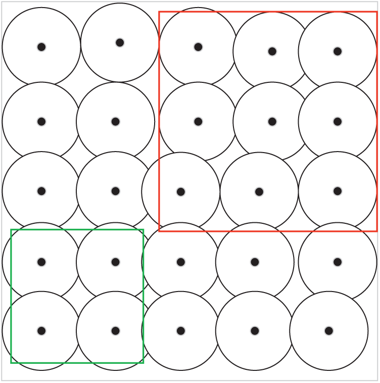
Figure 1: Schematic diagram of the monitoring region model

3  Determining the Mobile Nodes and Target Locations

To move the sensors reasonably, we employed the concentric circle method to move sensors in the non-key monitored areas to the key areas without changing the number of sensors. The sensors in the non-key monitored area were called mobile nodes and were located according to the grid nodes. The points with larger coverage holes in the key monitored area were called target locations, and their positions were determined as follows:

Suppose that the number of mobile nodes is less than the number of target locations.

Step 1. Determine the mobile nodes number N in the non-key monitored area.

Step 2. Determine the area that is not covered by the sensors. All grid points are taken as the center of the circle, and the width of the mesh is taken as the initial radius. Make concentric circles outward according to the grid width. The maximum radius of the concentric circle is the communication distance of the sensor.

Step 3. When the maximum ring of the concentric circle coincides with the coverage area the concentric circle radius will stop increasing.

Step 4. Assume that Q={q1,q2,…,qm} is the set of concentric circles of all grid nodes in the area that is not covered by the sensors, and find the circle with the largest radius in the set (if the maximum radii are the same, select the circle with the smaller sum of the horizontal and vertical coordinates of the center position). Record the node position and radius of the circle, and merge the area into the sensor coverage area.

Step 5. Repeat Steps (2)–(4). When the number of circles to be determined is equal to N, the process ends. Then the centers of these circles are the target locations.

4  Cascaded Movement Strategy Based on Floyd Algorithm

4.1 Cascaded Movement Strategy

After determining the point-to-point correspondence between the mobile nodes and the target locations, we determined how to move the mobile nodes to the target locations. Direct movement requires a long time, and long-distance movement of a single sensor will consume too much energy. The main idea of the cascaded movement strategy is to find some relay nodes to participate in the movement to reduce latency and balance the energy consumption. The principle of the cascaded movement strategy is shown in Fig. 2. Note that s0 is the node to be moved, and s1 and s2 are relay nodes. S0 moves to s1, and s1 moves to s2; then, s2 moves to s, where node s represents the target location. Nodes usually exchange their information logically, and then move simultaneously. By using the cascaded movement strategy, the time consumption was greatly reduced, and the energy originally consumed in s0 during the movement process was instead consumed by s0, s1, and s2. This method made the energy consumption of the sensor network more balanced. When selecting a cascaded movement path, we considered not only the total energy consumption but also the energy consumption of each sensor node. Therefore, we determined an optimal cascaded movement path.

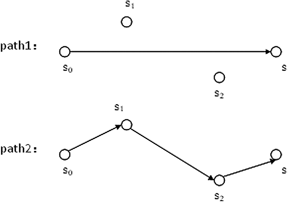
Figure 2: Cascaded movement

4.2 Floyd Algorithm

The Floyd algorithm can identify the shortest path between vertices in a given weighted graph [14–16]. In this study, we introduced the Floyd algorithm to the cascaded movement strategy. The sensors in the non-key monitored area were the initial points, and the target locations in the key area were the ending points. The remaining sensors were relay nodes. By calculating the shortest distance matrix and path matrix of the sensor nodes, and by backtracking the path matrix, we found the shortest distance of the sensor movement and the shortest cascaded path.

4.2.1 The Sensor Layout Model G=(V,E,C)

G=(V, E, C) is a weighted and directed graph, where V is the sensor node set, E is the set of the lines connected between nodes, and C is the distance adjacency matrix. In the sensor node set, v0,v1,…,vl represents l sensor nodes. The set E is formed by the nodes in V, where ek=[vivj] (the node vi is connected to node vj), and C is the distance adjacency matrix corresponding to graph G. cij is expressed as in Eq. (3):

cij={distance between vi and vjif(vi,vj)∈E0ifi=j∞if(vi,vj)∉E (3)

We constructed a suitable directed network graph to simulate the sensor network. The shortest path between the determined mobile node and the target location was planned by the Floyd algorithm, as shown in Fig. 3.

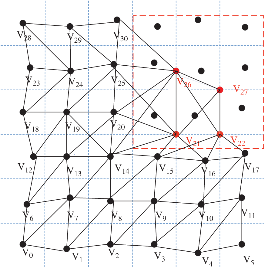
Figure 3: Sensor layout model

4.2.2 Model Description

This model regarded the sensor nodes in the non-key monitored area and the target locations in the key area as network nodes. The connected lines between the network nodes were abstracted as network edges and the relationship between these nodes was preserved.

The moving direction in the sensor networks was in a bidirectional path. The initial energy of the node and the actual distance of the path between the nodes should be comprehensively considered in the weights in application. Then, experts can label the weights. In this study, we considered only the distance.

4.2.3 Find the Shortest Distance Matrix D(n) and the Shortest Path Matrix R(n)

The basic idea of the Floyd algorithm is to construct v matrices D(1),D(2),…,D(v) in turn by inserting the points directly in the weighted adjacency matrix of the graph. The resulting matrix D(v) becomes the distance matrix of the graph, and the matrix of insertion points is calculated to obtain the shortest path between two points, where element dij0 of D(0) represents the distance between two connected nodes vi and vj (see Eq. (4)). D(k) and R(k) are calculated by Eqs. (5) and (6):

dij(0)={cijif(vi,vj)∈E0ifi=j∞if(vi,vj)∉E(4)

dij(k)=min{dij(k-1),dik(k-1)+dkj(k-1)}(i,j=1,2,…,n)(5)

rij(k)={kifdij(k-1)>dik(k-1)+dkj(k-1)rij(k-1)else(6)

We obtained the shortest distance matrix D(n) and the shortest path matrix R(n) by distance adjacency matrix C using the Floyd algorithm. Only the shortest path between the mobile node and the target location was saved in R(n). On this basis, the shortest path could be traced back to obtain the specific path between the two nodes. Then, according to the cascaded movement strategy, the mobile node was moved through the relay node to reach the target node location.

5  Simulation Analysis

5.1 Experimental Design

In this study, we used the cascaded movement strategy to move the sensors in the non-key monitored area to the key monitored area to achieve effective coverage of the key monitored areas. The water area was 100m×100 m, and the grid was 2m×2 m. The sensor radius was 10 m. The initial energy was 10000 J, and the energy consumption was 30 J when the sensor moved 1 m.

5.2 Experimental Results and Analysis

We increased the coverage of the key monitored areas by moving the sensors in the non-key monitored areas to the key monitored areas. Fig. 4 shows the distribution of sensor nodes after uniform deployment. The area enclosed in red represents the key monitored area, and the area enclosed by green indicates the non-key monitored area.

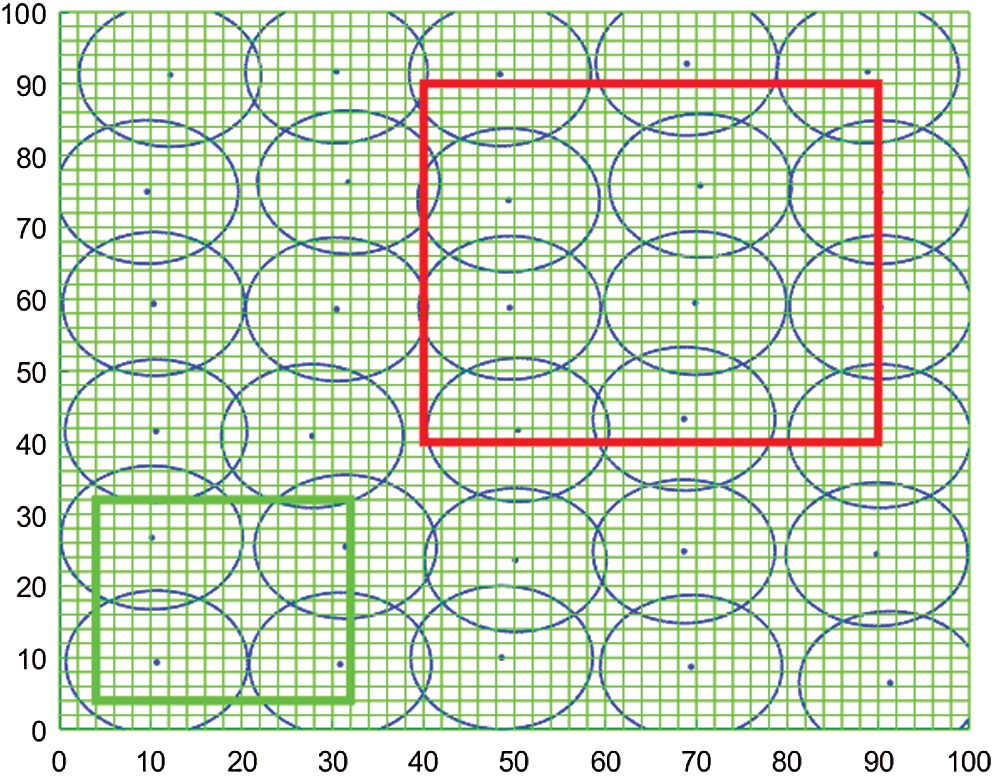
Figure 4: Distribution of the sensor nodes after uniform deployment

Fig. 5 presents the result of the final deployment of the sensors after cascaded movement. As shown in Fig. 5, the sensor nodes in the non-key monitored area have moved to the key monitored area, which greatly enhanced the coverage rate of the key monitored area.

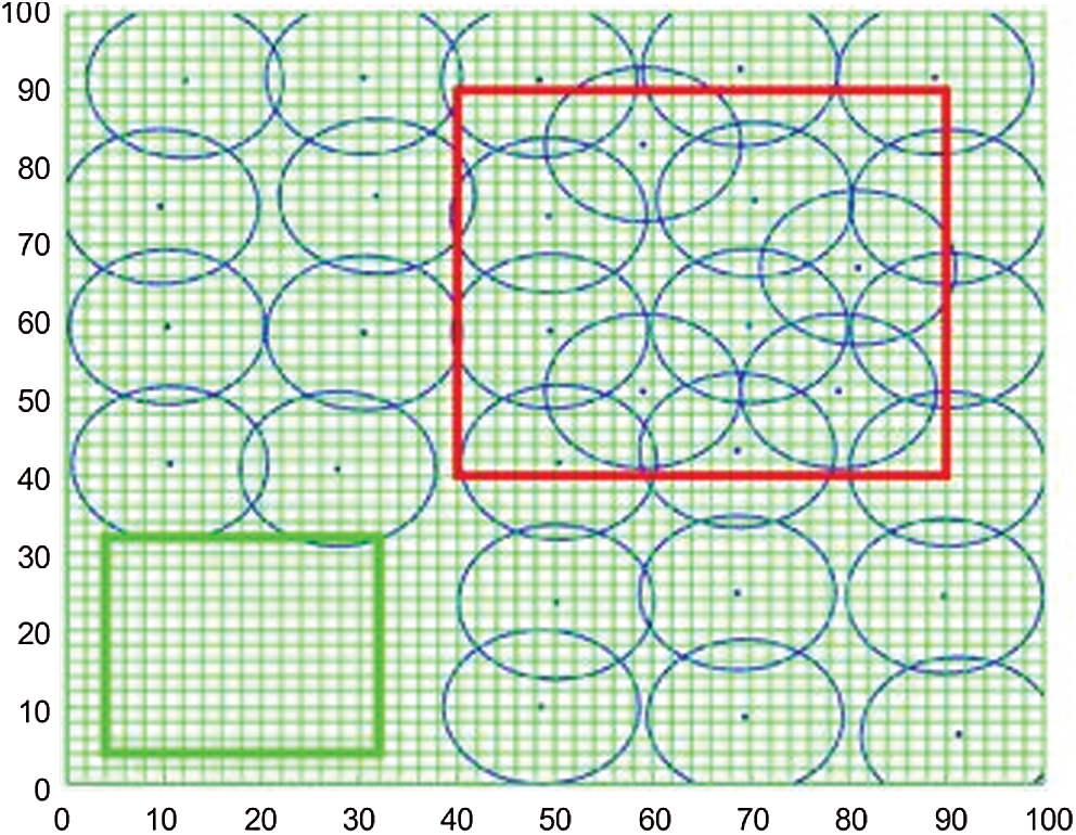
Figure 5: Distribution of the sensor nodes after cascaded movement

The change in coverage rate over time by direct movement is shown in Fig. 6. Fig. 7 presents the change in coverage rate with cascaded movement over time. With the movement of sensors in non-key monitored areas, the original uniform coverage was broken, which reduced the coverage of non-key monitored areas as well as the entire monitored area. At the same time, with the increase in sensor nodes in key monitored areas, the coverage of key monitored areas gradually increased, and eventually reached 96%. Thus, we achieved effective coverage of key monitored areas without increasing the number of sensors. Moreover, these two figures highlight that if we considered only the coverage rate, direct movement and cascaded movement were considered to be equivalent.

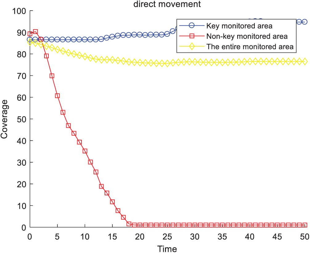
Figure 6: Coverage rate (direct movement)

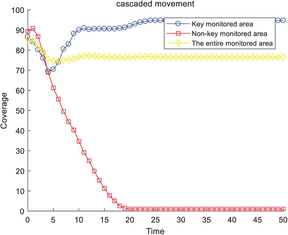
Figure 7: Coverage rate (cascaded movement)

Fig. 8 shows the total moved distance of the mobile sensor nodes when using direct movement and cascaded movement. We can see that when the sensor node reached a new balance (the growth of the coverage rate of key monitored area is less than 0.05%), the total move distance for the cascaded movement was slightly higher than that for the direct movement. We needed only 23.963 s, however, to reach the new balance for cascaded movement, whereas 35.012 s was required for direct movement. Therefore, using cascaded movement effectively reduced the network adjustment time.

Fig. 9 shows the nodes’ residual energy. Although direct movement could achieve effective coverage of key areas with less moved distance, some nodes’ residual energy was too low after moving. If we used cascaded movement, more nodes could be involved to share the energy consumption during the movement of sensor nodes. When the network reached a new balance, the residual energy of the nodes was relatively balanced, which effectively extended the life cycle of the network.

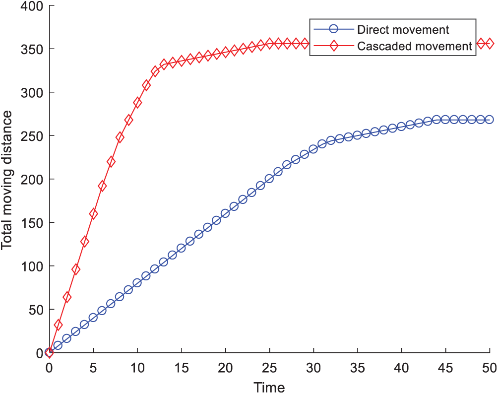
Figure 8: Moved distances

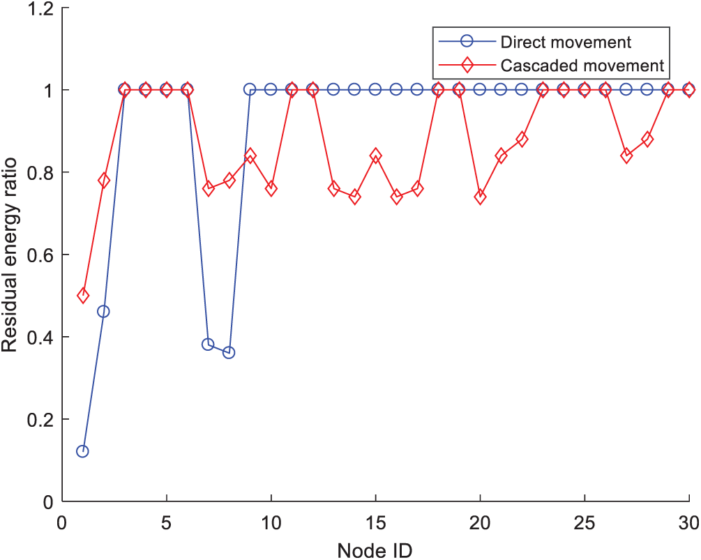
Figure 9: Residual energy of the sensor nodes

6  Conclusions

We studied the deployment of water quality sensor networks. First, we established the monitored area model and divided the entire monitored area into a key area and non-key area. The mobile nodes and the target locations were determined, and the cascaded movement strategy was used to move the sensors. This realized the effective coverage of the key monitored area under the condition of limited resources. The simulation results showed that the cascaded movement strategy could make the residual energy relatively balanced and extended the life cycle of the network compared with the direct movement.

Funding Statement: This research was funded by the National Natural Science Foundation of China (Grant No. 61802010); National Social Science Fund of China (Grant No. 19BGL184); Beijing Excellent Talent Training Support Project for Young Top-Notch Team (Grant No. 2018000026833TD01); and Hundred-Thousand-Ten Thousand Talents Project of Beijing (Grant No. 2020A28).

Conflicts of Interest: The authors declare that they have no conflicts of interest to report regarding the present study.

This work is licensed under a Creative Commons Attribution 4.0 International License, which permits unrestricted use, distribution, and reproduction in any medium, provided the original work is properly cited.