DOI:10.32604/cmc.2021.017046
| Computers, Materials & Continua DOI:10.32604/cmc.2021.017046 | |
| Article |
L-Moments Based Calibrated Variance Estimators Using Double Stratified Sampling
1Department of Mathematics and Statistics, International Islamic University, Islamabad, 44000, Pakistan
2Department of Mathematics and Statistics, PMAS-Arid Agriculture University, Rawalpindi, 46300, Pakistan
3Department of Mathematics, College of Science, King Khalid University, Abha, 62529, Saudi Arabia
4Statistical Research and Studies Support Unit, King Khalid University, Abha, 62529, Saudi Arabia
5Department of Mathematics, College of Science, Mustansiriyah University, Baghdad, 10011, Iraq
*Corresponding Author: Usman Shahzad. Email: usman.stat@yahoo.com
Received: 19 January 2021; Accepted: 04 March 2021
Abstract: Variance is one of the most vital measures of dispersion widely employed in practical aspects. A commonly used approach for variance estimation is the traditional method of moments that is strongly influenced by the presence of extreme values, and thus its results cannot be relied on. Finding momentum from Koyuncu’s recent work, the present paper focuses first on proposing two classes of variance estimators based on linear moments (L-moments), and then employing them with auxiliary data under double stratified sampling to introduce a new class of calibration variance estimators using important properties of L-moments (L-location, L-cv, L-variance). Three populations are taken into account to assess the efficiency of the new estimators. The first and second populations are concerned with artificial data, and the third populations is concerned with real data. The percentage relative efficiency of the proposed estimators over existing ones is evaluated. In the presence of extreme values, our findings depict the superiority and high efficiency of the proposed classes over traditional classes. Hence, when auxiliary data is available along with extreme values, the proposed classes of estimators may be implemented in an extensive variety of sampling surveys.
Keywords: Variance estimation; L-moments; calibration approach; double sampling; stratified random sampling
Planning is an integral part of the administrative process for the development of any field. Among the most important outputs of the planning process are the plans and programs that institutions seek to execute. One of the most important pillars of planning success is the availability of data and information that enables the decision-maker to conduct scientific analysis. In statistical literature, the additional information attached to each element is referred to as auxiliary (or ancillary, supplementary, supporting, concomitant) information. Whatever type of information is offered, it can be used to identify better sampling strategies. Auxiliary information has been used with sampling techniques for many years. The authors of [1,2] were pioneers in the usage of auxiliary information regarding the development of estimation techniques with high estimation accuracy. Recently, there have been many interesting works using auxiliary information in different ways [3–12].
In all sample surveys, the major concern is the derivation of point estimators for various parameters of interest. Nevertheless, it is equally important to evaluate the performance of these estimators. The importance of variance estimators lies primarily in the fact that the estimated variance, of any estimator, is a major component of its quality. Reference [13] pointed out that the importance of variance estimation lies in the fact that it offers an indicator of the quality of estimators. It can be used in calculating confidence intervals, and drawing accurate conclusions, and can provide indicators of data quality. The sampling design that underlies a sample survey is one of the most important factors determining both the size of sample and the procedure needed to estimate the variances. More specifically, there are many components of sample designs related to the estimation of variances, including the number of sampling stages. In single or one-stage sample designs, the stage is very direct, and the closed formula can be derived for estimation of variance. In designs with more than one stage, the state becomes complicated since there is more than one source of variance. At each stage, unit sampling (primary, secondary, etc.) leads to an additional component of variance. In cases where all other components of sampling and estimation are rather simple, a closed formula can be obtained by calculating the variance at each stage. However, common practice is to roughly estimate the variance by estimating the variation among the initial sampling units, since this is the dominant component of the overall variance. For example, with double or two-stage sampling, there are two sources of variance such as variation resulting from the selection of the primary sampling units and the variation resulting from the selection of the secondary sampling units (for more details, see [14]). There are also many studies that have employed double sampling for real data [15–18]. In this paper, we consider double stratified random sampling. With stratified sampling, the population is split into subpopulations that are not overlapping; these are known as strata and typically describe homogeneous subpopulations, resulting in reduced overall variability. A random sample is chosen from each stratum, independently of the other stratum. A stratified sampling pattern may be the same or different from that of other stratum.
Consider
It is worth noting that
The analysis of sample data is complex. The complexity of the analysis increases when the data contains unusual points (outliers or extreme values) that affect the robustness of the variance estimation under traditional central moments. One of the solutions to tackle this issue is to use L-moments instead of traditional central moments. L-moments provide a robust statistical framework for the analysis. L-moments [19] are determined by linear combinations of the expected values of the order statistics (O.S.). Furthermore, calibration estimation is another common statistical approach that relies on the use of auxiliary information to adjust the original weights of the design and improve the accuracy of estimators. The authors of [20] were pioneers in the use of calibration estimation with survey data and several additional works on mean estimation have been published since (for example, see [21–23]).
In the present paper, our objective is to develop some new classes of variance estimators for a variable of interest, based on L-moments and the calibration approach under double stratified random sampling. The remainder of this article is organized as follows. In Section 2, the L-moments and proposed classes are presented in detail. Numerical illustrations of three populations are offered in Section 3 to evaluate the performance of the new estimators. Finally, Section 4 provides conclusions.
2 L-Moments and Proposed Classes
Reference [19] described the L-moments as expectations of the order statistics of certain linear combinations. L-moments can be specified for any random variable for which a mean exists. They are used to describe probability distributions and estimate parameters, and their estimates are used for summarizing and describing the samples of observed data. There are many advantages of L-moments over traditional moments: they are linear data functions, they suffer less from the effects of sample change-ability, they are more robust to outliers/extreme values in data, and they enable safer inferences made from small samples about any fundamental population parameter. The general population mathematical forms of first four L-moments for the auxiliary variable X in relation to the stratum h are defined as follows:
Similarly, we can write second-stage sample L-moments of the auxiliary variable as
2.1 First Proposed Class of Estimators
The authors of [9,10] used robust regression and robust co-variance matrices methodologies for improved estimation of the population’s mean. Their use of robust regression and robust co-variance matrices allows us to utilize robust moments (L-moments) instead of traditional moments. Hence, taking motivation from [21], we propose the following class of L-moments based calibration estimators of variance under double stratified sampling:
where the calibrated weights are selected to minimize the measure of chi-square distance
is subject to the following calibration constraints
where
The Lagrange function is given as
where
Now,
By substituting the value of
where
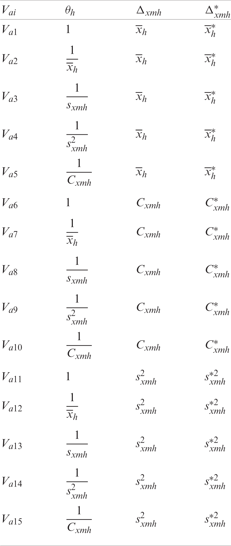
The members of the first proposed class are provided in Tab. 1.
Table 1: First proposed class of estimators
2.2 Second Proposed Class of Estimators
By extending the idea of Vai, we propose the second class of estimators of variance under double stratified sampling as given below:
Through using the distance of chi-square,
which is subject to the following three calibration constraints:
The Lagrange function is given as
After taking the derivative of T with respect to
The following equations system can be obtained by substituting Eq. (16) into Eqs. (13)–(15) respectively:
Upon solving the equations system for
When substituting these
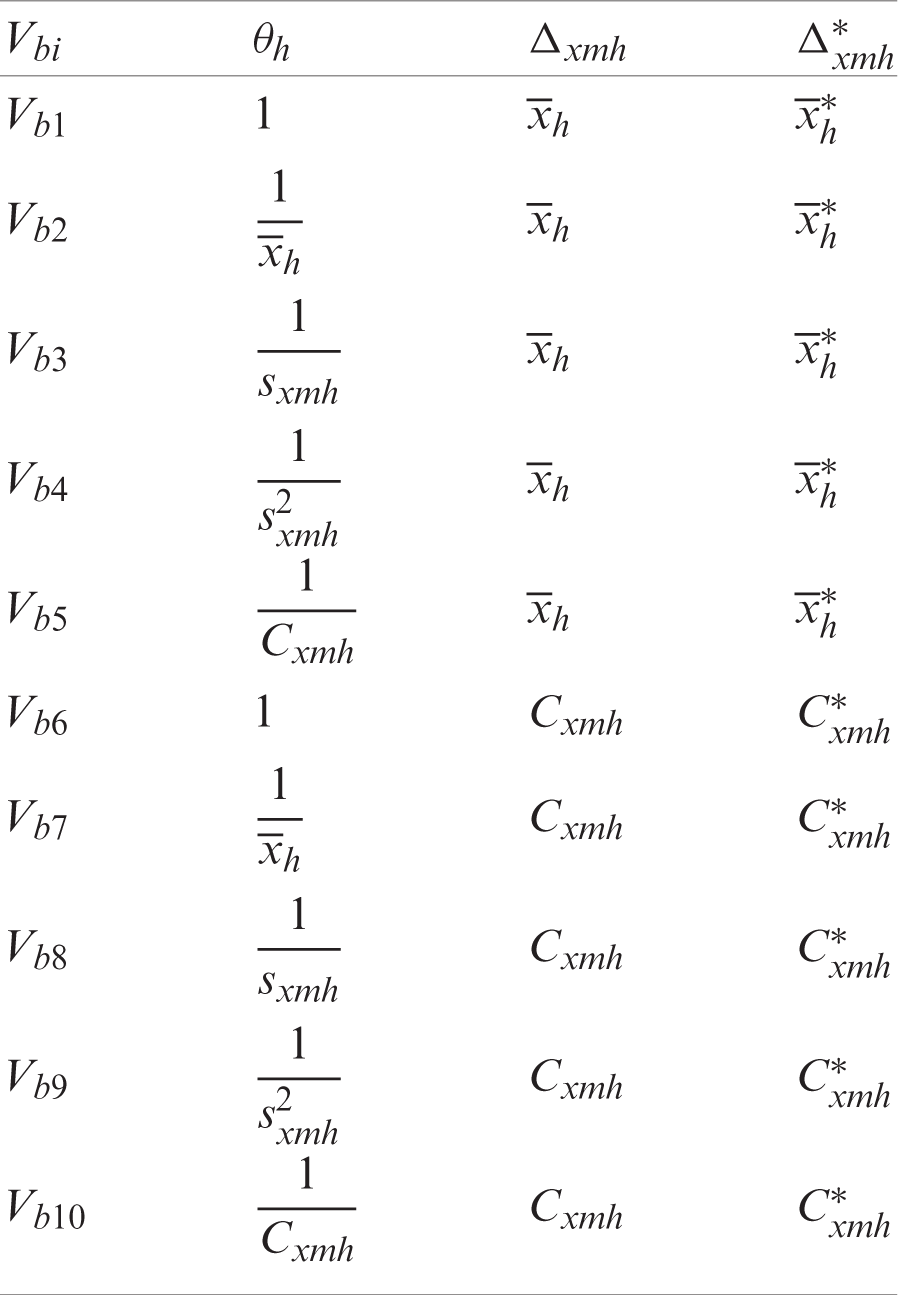
The members of the second proposed class are listed in Tab. 2.
Table 2: Second proposed class of estimators
Here, we evaluate the performance of the proposed estimators through three populations.
3.1 Simulation Design (Population-1)
In this article, we consider the population with size
where
Figs. 1–4 show the scatter plots for each stratum. The existence of extreme values is clearly demonstrated by these figures and are therefore fitting for evaluating our proposed estimators.
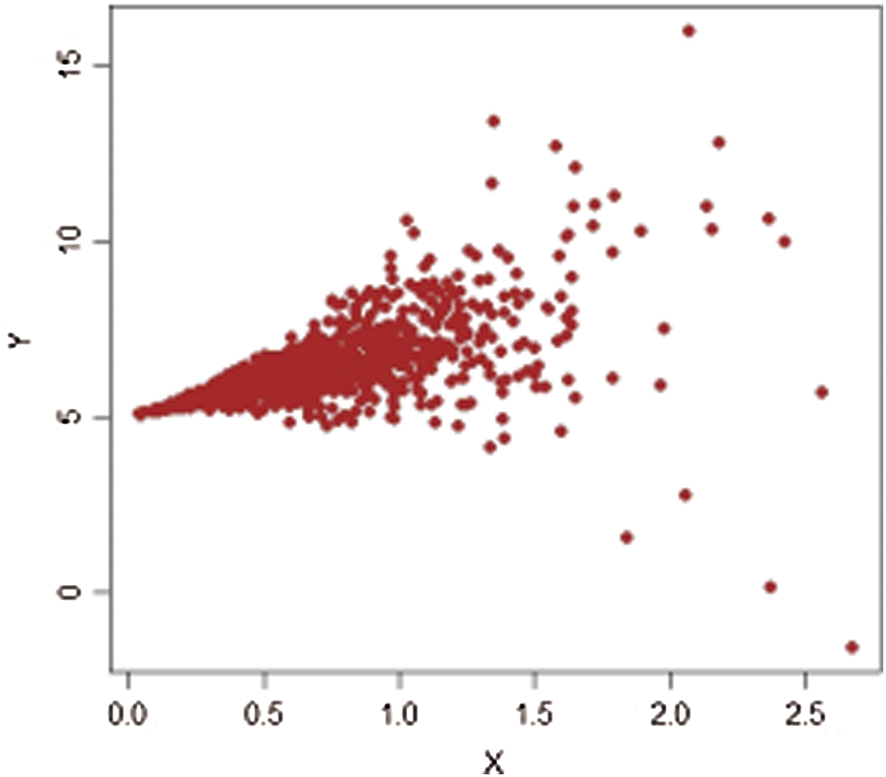
Figure 1: Population-1,
The simulation steps are as below:
Step 1: Select a random sample with size nh through SRSWOR from stratum h.
Step 2: Find the value of variance estimate, say
Step 3: Repeat Steps 1 and 2 for L = 5000 times. Obtain
Step 4: Compute the mean square error (MSE) as
Step 5: Compute the percentage relative efficiency (PRE) as
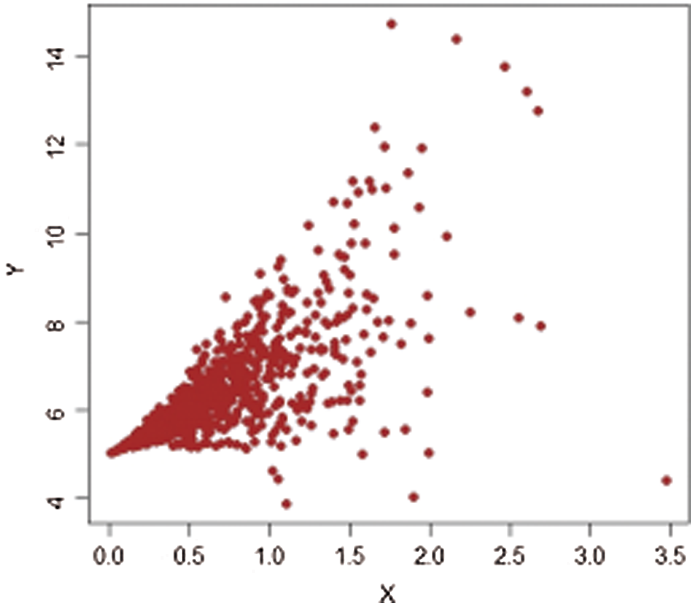
Figure 2: Population-1,
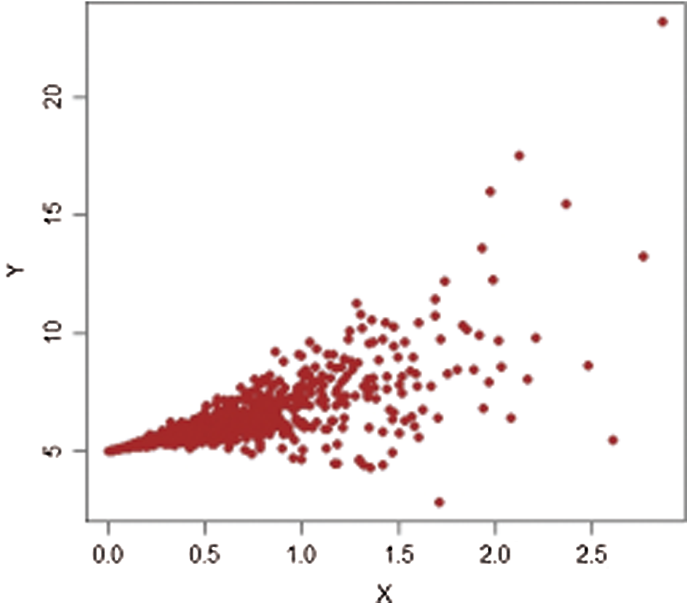
Figure 3: Population-1,
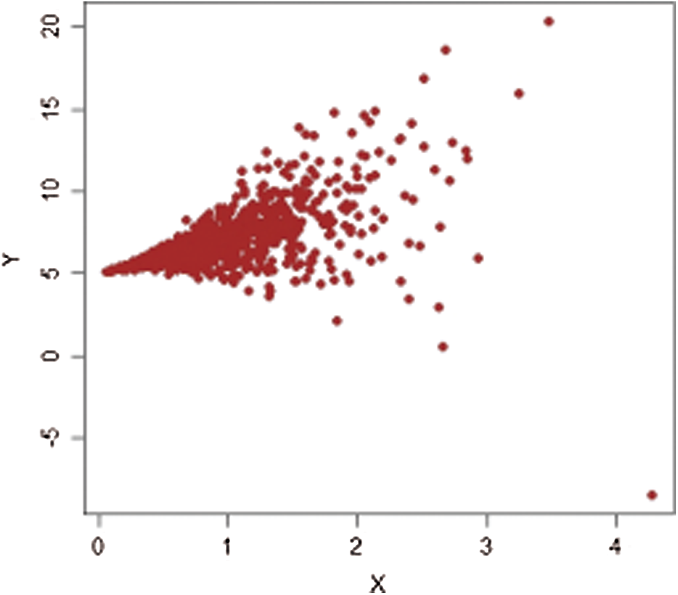
Figure 4: Population-1,
The estimators’ PRE obtained from the above five steps are provided in Tab. 3.
The apple fruit is one of the most common types of fruits. It is native to Central Asia, but today it grows worldwide with different colors and sizes. The apple fruit is rich in fiber, vitamins, and antioxidants and has many health benefits.
In the present article, we use collected apple fruit data used by [24], where
Population-2:
Population-3:
It should be noted that we consider 477 villages in four strata in 1999, termed (1: Marmarian), (2: Agean), (3: Mediterranean), and (4: Central Anatolia). The scatter plots of extreme values for each stratum are shown in Figs. 5–12. The estimators’ PREs are computed as defined in Subsection 3.1, and are presented in Tabs. 4 and 5. The first-stage samples with sizes
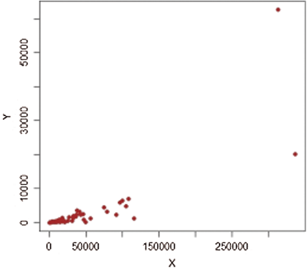
Figure 5: Population-2,
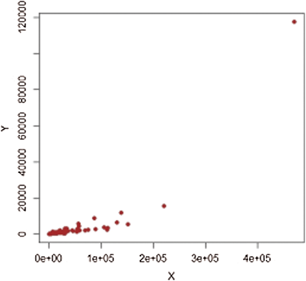
Figure 6: Population-2,

Figure 7: Population-2,
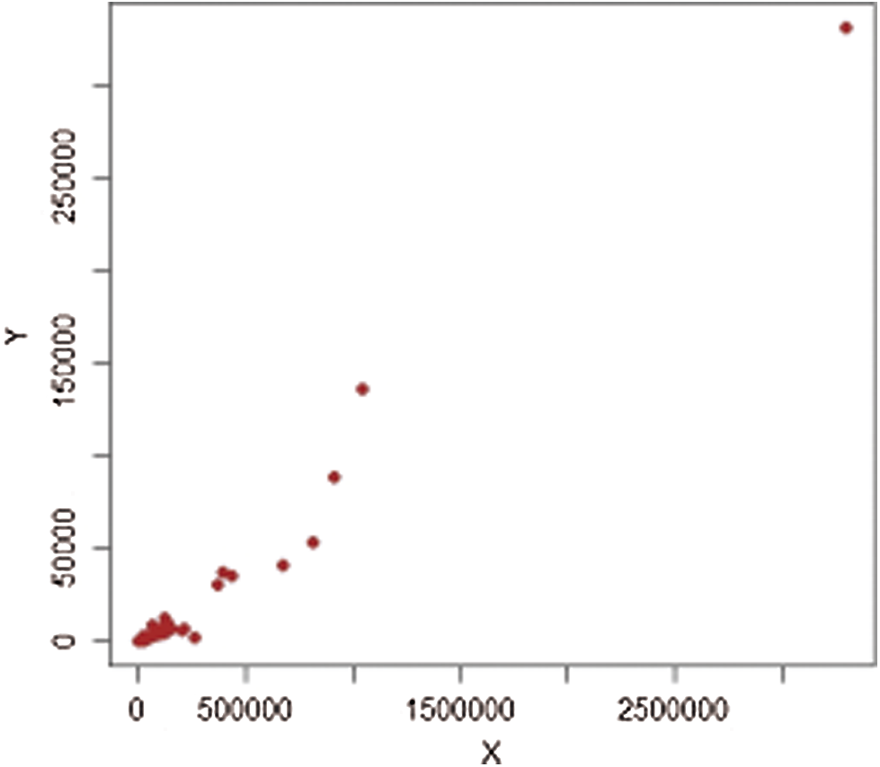
Figure 8: Population-2,
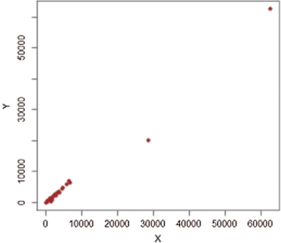
Figure 9: Population-3,
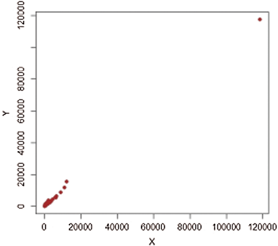
Figure 10: Population-3,
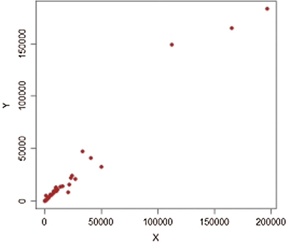
Figure 11: Population-3,
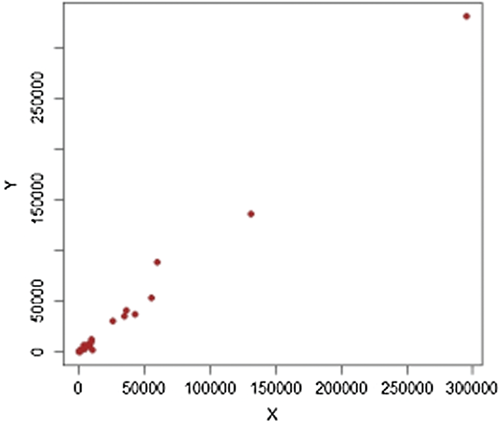
Figure 12: Population-3,
1: From Tab. 3, we can see that the results
The proposed estimators Va11 and Vb3 record the highest efficiency compared to other competitor estimators.
2: Meanwhile, the results
The proposed estimators Va11 and Vb5 record the highest efficiency compared to other competitor estimators.
3: The results
Hence, the proposed estimators Va11 and Vb1 record the highest efficiency of all compared estimators.
4: Comparing the two proposed classes for each population, leads us to the following findings:
Population-1:
Population-2:
Population-3:
5: Overall, all the members of new classes have PRE > 100 with respect to To, and this clearly indicates that the performance of the proposed estimators is better than that of traditional estimators.
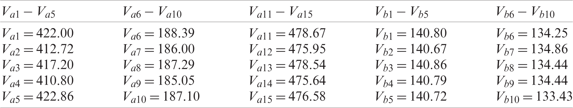
6: Furthermore, the proposed variance estimator Va11 is the best estimator among all proposed estimators, having PREs of 478.67, 28051.41, and 77307.88 for populations 1–3, respectively.
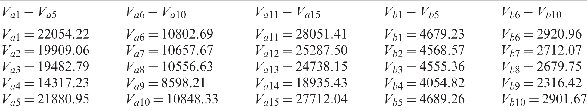
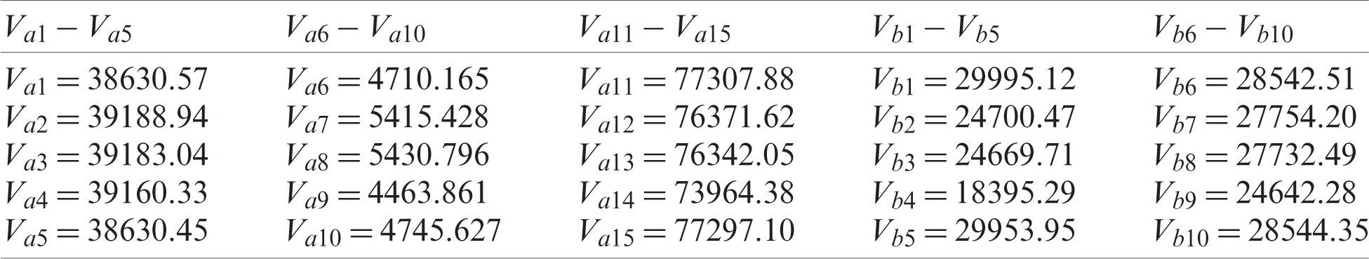
The difficulty of data analysis arises from the presence of extreme values that adversely impact the variance estimation based on central moments. One of the ways to solve this issue is to use L-moments that provide a robust statistical structure for analysis. Calibration estimation is a common statistical approach that relies on the use of auxiliary information to adjust the original weights of design and to improve the accuracy of estimators. Motivation by [21], we propose new classes of estimators to estimate the population variance based on L-moments and present a calibration approach for double stratified random sampling. The percentage relative efficiency is adopted to compare the performance of the proposed estimators through three populations and through a simulation as well as application to real-life data. Our numerical results show that the proposed estimators are always superior and more efficient to existing estimators.
Funding Statement: The authors thank the Deanship of Scientific Research at King Khalid University, Kingdom of Saudi Arabia for funding this study through the research groups program under Project Number R.G.P.1/64/42. Ishfaq Ahmad and Ibrahim Mufrah Almanjahie received the grant.
Conflicts of Interest: The authors declare that they have no conflicts of interest to report regarding the present study.
1. D. J. Watson, “The estimation of leaf area in field crops,” Journal of Agricultural Science, vol. 27, no. 3, pp. 474–483, 1937. [Google Scholar]
2. W. G. Cochran, “The estimation of the yields of cereal experiments by sampling for the ratio of grain to total produce,” Journal of Agricultural Science, vol. 30, no. 2, pp. 262–275, 1940. [Google Scholar]
3. K. Ibrahim, M. Syam and A. I. Al-Omari, “Estimating the population mean using stratified median ranked set sampling,” Applied Mathematical Sciences, vol. 4, no. 47, pp. 2341–2354, 2010. [Google Scholar]
4. M. Syam, K. Ibrahim and A. I. Al-Omari, “The efficiency of stratified quartile ranked set sample in estimating the population mean,” Tamsui Oxford Journal of Information and Mathematical Sciences, vol. 28, no. 2, pp. 175–190, 2012. [Google Scholar]
5. M. Abid, N. Abbas and M. Riaz, “Improved modified ratio estimators of population mean based on deciles,” Chiang Mai Journal of Science, vol. 43, no. 1, pp. 1311–1323, 2016. [Google Scholar]
6. U. Shahzad, P. F. Perri and M. Hanif, “A new class of ratio-type estimators for improving mean estimation of nonsensitive and sensitive variables by using supplementary information,” Communications in Statistics-Simulation and Computation, vol. 48, no. 9, pp. 2566–2585, 2019. [Google Scholar]
7. N. Ali, I. Ahmad, M. Hanif and U. Shahzad, “Robust-regression-type estimators for improving mean estimation of sensitive variables by using auxiliary information,” Communications in Statistics—Theory and Methods, vol. 50, no. 4, pp. 979–992, 2019. [Google Scholar]
8. M. Hanif and U. Shahzad, “Estimatıon of population variance using kernel matrix,” Journal of Statistics and Management Systems, vol. 22, no. 3, pp. 563–586, 2019. [Google Scholar]
9. T. Zaman and H. Bulut, “Modified ratio estimators using robust regression methods,” Communications in Statistics-Theory and Methods, vol. 48, no. 8, pp. 2039–2048, 2019. [Google Scholar]
10. T. Zaman and H. Bulut, “Modified regression estimators using robust regression methods and covariance matrices in stratified random sampling,” Communications in Statistics-Theory and Methods, vol. 49, no. 14, pp. 3407–3420, 2020. [Google Scholar]
11. U. Shahzad, N. H. Al-Noor, M. Hanif and I. Sajjad, “An exponential family of median based estimators for mean estimation with simple random sampling scheme,” Communications in Statistics-Theory and Methods, vol. 43, no. 1, pp. 1–10, 2020. [Google Scholar]
12. U. Shahzad, N. H. Al-Noor, M. Hanif, I. Sajjad and A. M. Muhammad, “Imputation based mean estimators in case of missing data utilizing robust regression and variance-covariance matrices,” Communications in Statistics-Simulation and Computation, vol. 3, no. 2, pp. 1–20, 2020. [Google Scholar]
13. F. Gagnon, H. Lee, E. Rancourt and C. E. Särndal, “Estimating the variance of the generalised regression estimator in the presence of imputation for the generalised estimation system,” in Proc. of the Survey Methods Section, Statistical Society of Canada, pp. 151–156, 1996. [Google Scholar]
14. C. E. Särndal, B. Swensson and J. Wretman, Model Assisted Survey Sampling. New York: Springer-Verlang, 1992. [Google Scholar]
15. A. A. Jemain, A. I. Al-Omari and K. Ibrahim, “Modified ratio estimator for the population mean using double median ranked set sampling,” Pakistan Journal of Statistics, vol. 24, no. 3, pp. 217–226, 2008. [Google Scholar]
16. A. I. Al-Omari, “Ratio estimation of the population mean using auxiliary information in simple random sampling and median ranked set sampling,” Statistics and Probability Letters, vol. 82, no. 11, pp. 1883–1890, 2012. [Google Scholar]
17. M. Syam, K. Ibrahim and A. I. Al-Omari, “The efficiency of stratified double percentile ranked set sample for estimating the population mean,” Far East Journal of Mathematical Sciences, vol. 73, no. 1, pp. 157–177, 2013. [Google Scholar]
18. M. Syam, A. I. Al-Omari and K. Ibrahim, “On the mean estimation using stratified double median ranked set sampling,” American Journal of Applied Sciences, vol. 14, no. 4, pp. 496–502, 2017. [Google Scholar]
19. J. R. Hosking, “L-moments: Analysis and estimation of distributions using linear combinations of order statistics,” Journal of the Royal Statistical Society: Series B (Methodological), vol. 52, no. 1, pp. 105–124, 1990. [Google Scholar]
20. J. C. Deville and C. E. Särndal, “Calibration estimators in survey sampling,” Journal of the American Statistical Association, vol. 87, no. 418, pp. 376–382, 1992. [Google Scholar]
21. N. Koyuncu, “Calibration estimator of population mean under stratified ranked set sampling design,” Communications in Statistics-Theory and Methods, vol. 47, no. 23, pp. 5845–5853, 2018. [Google Scholar]
22. U. Shahzad, I. Ahmad, I. Almanjahie, N. H. Al-Noor and M. Hanif, “A new class of L-moments based calibration variance estimators,” Computers Materials and Continua, vol. 66, no. 3, pp. 3013–3028, 2021. [Google Scholar]
23. U. Shahzad, I. Ahmad, I. Almanjahie, M. Hanif and N. H. Al-Noor, “L-moments and calibration based variance estimators under double stratified random sampling scheme: An application of covid-19 pandemic,” Scientia Iranica, pp. 1–17, 2021. [Google Scholar]
24. N. Koyuncu and C. Kadilar, “Ratio and product estimators in stratified random sampling,” Journal of Statistical Planning and Inference, vol. 139, no. 8, pp. 2552–2558, 2009. [Google Scholar]
 | This work is licensed under a Creative Commons Attribution 4.0 International License, which permits unrestricted use, distribution, and reproduction in any medium, provided the original work is properly cited. |