DOI:10.32604/cmc.2021.016881
| Computers, Materials & Continua DOI:10.32604/cmc.2021.016881 | |
| Article |
Bitcoin Candlestick Prediction with Deep Neural Networks Based on Real Time Data
1Department of Information Technology, College of Computer, Qassim University, Buraydah, 51452, Saudi Arabia
2Department of Computer Science, College of Computer, Qassim University, Buraydah, 51452, Saudi Arabia
*Corresponding Author: Amal A. Al-Shargabi. Email: a.alshargabi@qu.edu.sa
Received: 14 January 2021; Accepted: 26 February 2021
Abstract: Currently, Bitcoin is the world’s most popular cryptocurrency. The price of Bitcoin is extremely volatile, which can be described as high-benefit and high-risk. To minimize the risk involved, a means of more accurately predicting the Bitcoin price is required. Most of the existing studies of Bitcoin prediction are based on historical (i.e., benchmark) data, without considering the real-time (i.e., live) data. To mitigate the issue of price volatility and achieve more precise outcomes, this study suggests using historical and real-time data to predict the Bitcoin candlestick—or open, high, low, and close (OHLC)—prices. Seeking a better prediction model, the present study proposes time series-based deep learning models. In particular, two deep learning algorithms were applied, namely, long short-term memory (LSTM) and gated recurrent unit (GRU). Using real-time data, the Bitcoin candlesticks were predicted for three intervals: the next 4 h, the next 12 h, and the next 24 h. The results showed that the best-performing model was the LSTM-based model with the 4-h interval. In particular, this model achieved a stellar performance with a mean absolute percentage error (MAPE) of 0.63, a root mean square error (RMSE) of 0.0009, a mean square error (MSE) of 9e-07, a mean absolute error (MAE) of 0.0005, and an R-squared coefficient (R2) of 0.994. With these results, the proposed prediction model has demonstrated its efficiency over the models proposed in previous studies. The findings of this study have considerable implications in the business field, as the proposed model can assist investors and traders in precisely identifying Bitcoin sales and buying opportunities.
Keywords: Bitcoin; prediction; long short term memory; gated recurrent unit; deep neural networks; real-time data
Recently, virtual currency has gained more popularity as an accepted means for financial transactions. The cryptocurrencies are the most representative virtual currencies and receive more attention from the media and investors [1,2]. This is due to their attractive characteristics, such as simplicity, transparency, and increasing acceptance [3]. Bitcoin is the first and the most popular cryptocurrency on the market. It was implemented by Nakamoto [4] in January 2009 and is currently traded on over 40 exchanges worldwide and acceptable in over thirty different currencies [5].
Bitcoin allows people to sell and buy using different currencies. Bitcoins do not necessitate an institution or central bank to emit and control them. Therefore, the decentralization of Bitcoins makes possessors of Bitcoins feel safe. As Bitcoin is grounded on Blockchain as its primary database, it has some anonymity features. The username of a Bitcoin user is not disclosed during transactions; only their wallet ID is made public. Such features have made Bitcoin one of the most commonly used and valuable cryptocurrencies. Thus, Bitcoin is rising and has become an attractive investment for traders [6]. For traders or general users, the main issue is the Bitcoin exchange rate volatility. As Van Alstyne [7] mentioned, the excessive volatility of Bitcoin is a factor that prevents it being a currency; however, this volatility is thus far a motivation for traders. Meanwhile, the general public are seeking solutions to cut down their risk. In fact, the Bitcoin price is remarkably volatile and changeable within a very short period of time.
To provide a better picture of this dilemma, Fig. 1 shows a sample of the fluctuations in Bitcoin’s price within a single day, i.e., May 10, 2020.
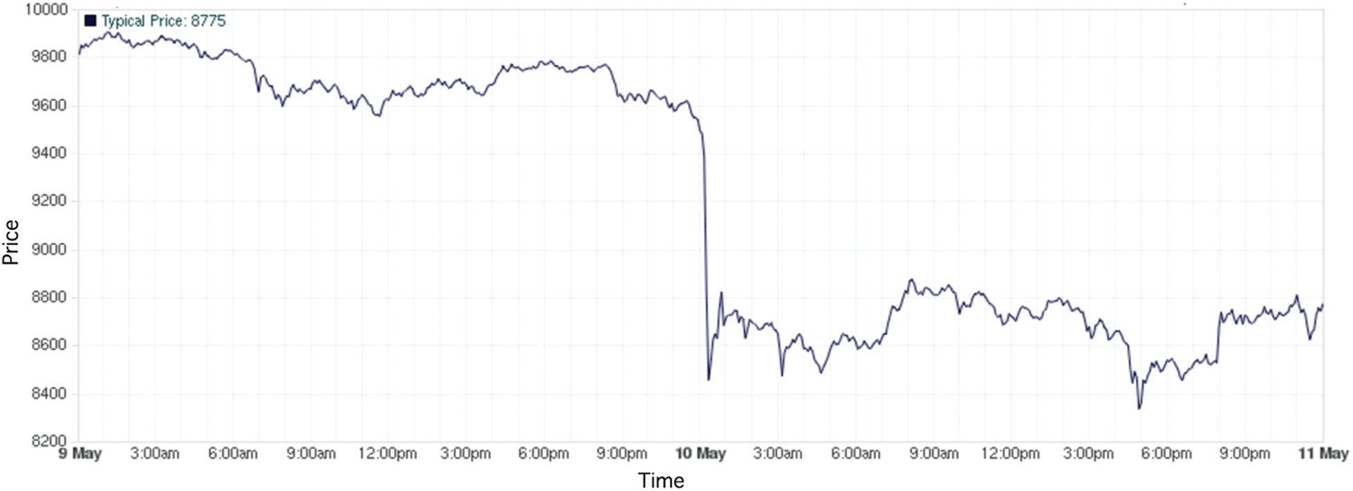
Figure 1: A sample of fluctuating Bitcoin price (in USD) collected from Bitstamp (https://www.bitstamp.net). Price was very volatile on 10 May 2020 and fell from 9,561 to 8,293 USD
As shown in Fig. 1, the recorded Bitcoin price was 9,561 USD at the beginning of the day and dropped down to 8,293 USD before the end of the same day. That is, the price dropped by around 13% within one single day.
In the financial world, the opportunity to predict the price direction of assets is a practical matter that helps a trader decision to buy or sell an investment instrument. Given that Bitcoin has a relatively young lifespan and volatile approach, there currently exists a novel opportunity to predict its price.
Existing studies of cryptocurrency and Bitcoin prediction, mostly short-term prediction, are mainly based on historical data, i.e., benchmark data, and many of these studies provide a relatively low-performance prediction. We assume that one of the main reasons for inaccurate prediction is the dependency on historical datasets. Bitcoin price time series data are typically collected from the past without taking into account the real-time (i.e., live) data. This is because the Bitcoin price readings for a few days may make a difference due to the price volatility problem mentioned earlier.
The majority of Bitcoin prediction studies mainly focus on using different algorithms on prediction performance alone rather than the effect of data type (historical vs real-time data) on prediction performance. To our knowledge, the present study is the first to compare Bitcoin prediction performance of historical data with real-time data. Specifically, this study starts with the collection of a dataset of real-time Bitcoin candlesticks from popular resources such as BitcoinCharts (https://bitcoincharts.com) and CryptoCompare (https://www.cryptocompare.com). The candlestick refers to four Bitcoin attributes: opening price, highest price, lowest price, and closing price, over a period of time, i.e., OHLC. With a historical dataset, the collected dataset is used to train two deep learning models: LSTM and GRU. These two models were selected due to their appropriateness to time series data. Three time intervals are used to develop the best-fit model: 4, 12, and 24-h intervals. The trained models are tested, and their performances are measured to identify the best-performed model. For evaluation, the best-performing model is compared with previous models in terms of performance.
The main contributions of this study are as follows: 1) The use of both historical and real-time data for the Bitcoin candlesticks prediction. The use of real-time data was not emphasized in previous studies, e.g., [5]. The majority of the studies were mainly based on historical-based data, 2) The proposal of multiple prediction models, i.e., LSTM and GRU. In literature, several models have been applied. However, the use of numerous deep learning methods in a single study was not common. In particular, the use of long short term memory (LSTM) together with the gated recurrent unit (GRU) was not widely used for Bitcoin price prediction, and 3) The consideration of three intervals in the prediction, i.e., 4, 12, 24-h. The proposal of three intervals gives more flexibility for people to choose sales and buy opportunities at different times.
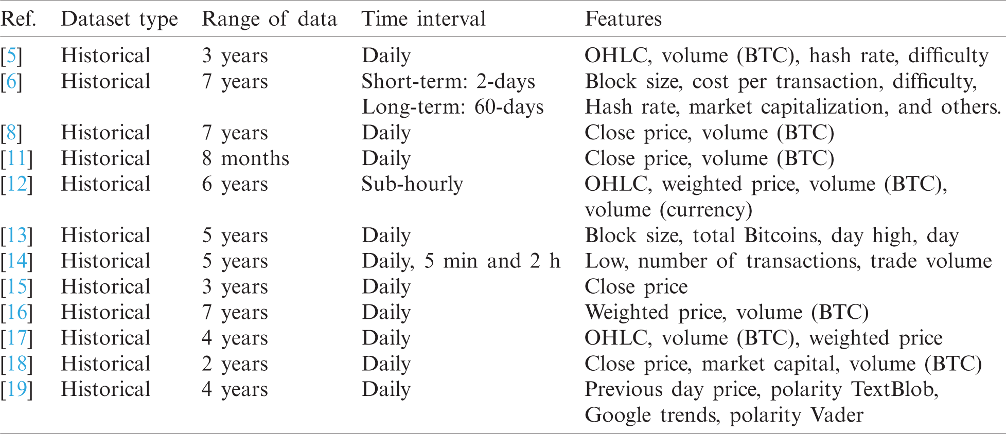
Tab. 1 shows a summary of related studies, in terms of the type of the Bitcoin dataset type used for prediction, i.e., historical vs. real-time, and the Bitcoin features used for prediction. As shown in the table, almost all studies depend on historical data and do not consider real-time data when building their prediction models. However, these studies make use of a wide variety of features. The features can be classified into two main categories: primary and secondary. The primary features are those related directly to Bitcoin and Blockchain per se and can affect the short-term Bitcoin price. These include examples like open price, daily high, hash rate, and block size. In contrast, the secondary features are loosely related to the Bitcoin and can affect the long-term Bitcoin price, such as international exchange rates, microeconomic, and technical indicators. Most of the studies used the primary features. As in the study of Shintate et al. [8], the author uses the open, high, low, and close of Bitcoin as the main features to build a new trend prediction classification method for Bitcoin price. The same study relied on a pre-processing phase before data analysis. They proposed a deep learning-based random sampling model (RMS) for cryptocurrency time series that are non-stationary. Also, the study of Purbarani et al. [9] applied Pearson correlation to select the most correlated features and found that OHLC were the most correlated features to predict the weighted price of Bitcoin.
Several approaches have been applied in the context of prediction methods, such as time series analysis, traditional machine learning algorithms, and deep learning algorithms. Madan et al. [10] compare forecasting Bitcoin price accuracy through binomial logistic regression, random forest, and support vector machine. Wu et al. [11] propose a new prediction framework using the LSTM model to predict Bitcoin’s daily price with two distinct LSTM models: a conventional LSTM model and an LSTM with an autoregressive model. Phaladisailoed et al. [12] applied different models, such as gated recurrent unit (GRU), Huber regression, LSTM, and Theil-Sen regression. The first model, GRU, shows the best results in which the means square error (MSE) was as low as 0.00002, and the R-squared coefficient (R2) was as high as 99.2%.
Table 1: summary of related Bitcoin prediction studies
Despite the importance of Bitcoin price prediction approaches, two main limitations can be derived from the literature. First, most Bitcoin studies focus on the security aspects rather than creating efficient prediction models for the Bitcoin price. Second, among the limited number of Bitcoin price prediction studies, most of the studies used historical datasets as they mainly focused on developing new models for prediction rather than studying the effect of the dataset (i.e., historical or real-time) on the prediction performance.
To bridge this gap, this study proposes prediction models for the Bitcoin candlestick and compares Bitcoin prediction performance of historical data with real-time data.
3 The Proposed Real-Time Prediction Model of Bitcoin Candlestick
In this section, the proposed model of Bitcoin price prediction is described. Fig. 2 shows the proposed model. First, the real-time data of Bitcoin candlesticks are collected with particular features (Section 3.1). The datasets collected are for three intervals: 4, 12, and 24 h. Second, the collected data are pre-processed before feeding them to the prediction models. The pre-processing includes cleaning data, such as removing outliers and fixing missing values, and also a transformation of data using data normalization (Section 3.2). Third, the prediction models are built with specific configurations. The models created are LSTM and GRU, which are deep learning-based models appropriate to be used with time-series data. The two models are constructed with specific structures to achieve good performance (Section 3.3). The models are trained based on the real-time data collection, and the performance of the models is evaluated in terms of specific metrics (Section 3.4). An experiment is conducted based on the phases included in the proposed model. The experiment is explained in detail in the following sub-sections.
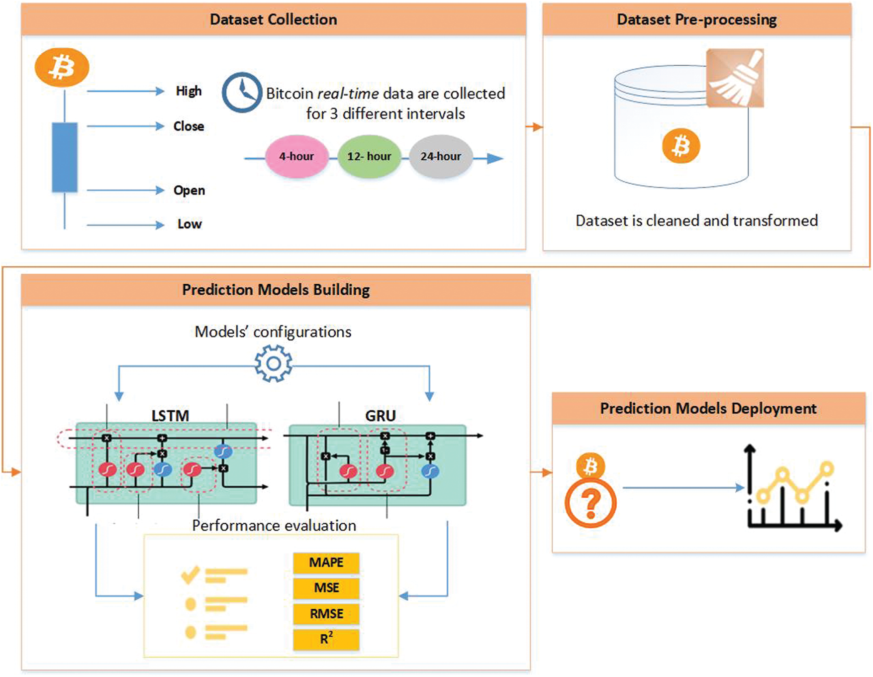
Figure 2: The proposed real-time prediction model of Bitcoin candlestick
The collection of data followed two steps. First, the historical data of Bitcoin were scraped from BitcoinCharts (https://bitcoincharts.com) for the period of January 1, 2017 to August 20, 2020. Next, the live, i.e., real-time data were requested from CryptoCompare (https://www.cryptocompare.com) websites using APIs from August 21, 2020, up to the current date, which on August 27, 2020 was streamed. The data were collected over 1-min intervals of Kraken exchange activity in US dollars. The collected data were then used to create three intervals: 4, 12, and 24 h. These intervals are made to get multiple alternatives in the prediction process.
Tab. 2 shows the key features considered: those representing the Bitcoin candlestick, opening price, highest price, lowest price, and closing price, i.e., OHLC. The final dataset collected has over 1,300,000 rows with a size of 120 MB, growing each time we request the API.
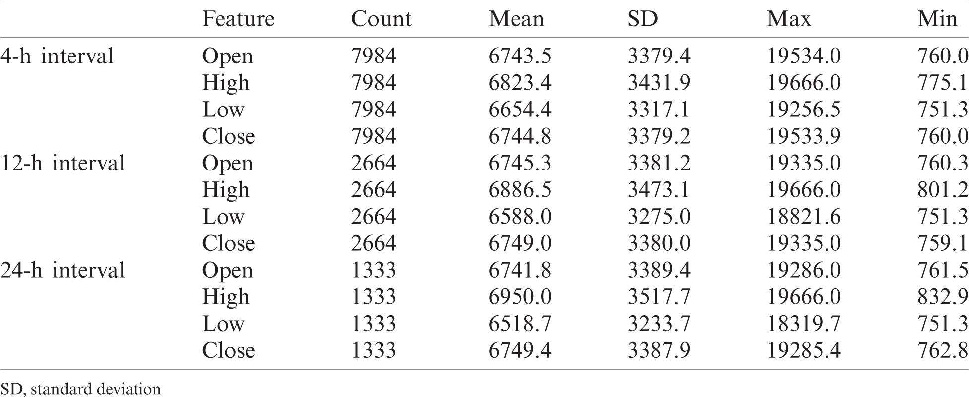
To get an overview of the collected dataset, Tab. 3 shows descriptive statistics of the features within three intervals: 4, 12, and 24 h. Note that as the interval is longer, the number of records is reduced.
Table 2: Features included in the dataset with their descriptions
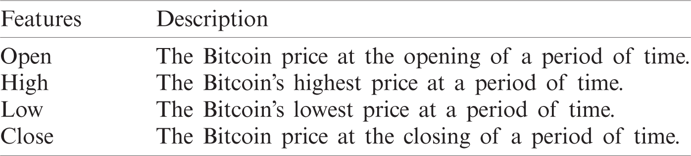
Table 3: Descriptive statistics Bitcoin features utilized for prediction. Statistics include the number of dataset records (samples) in each interval, the mean, the standard deviation, the maximum value, and the minimum value of each feature
To understand the data more, Fig. 3 shows how Bitcoin candlestick prices change over time. As shown in the figure, the OHLC features are similar in terms of the trend, but with different values.
As the dataset came from two sources, i.e., BitcoinCharts (https://bitcoincharts.com) and CryptoCompare (https://www.cryptocompare.com/), the processing step is significant since each source provides different features in a different order. To guarantee the correctness and consistency of the dataset, pre-processing methods have been applied, such as excluding the outliers and the null values, deleting irrelevant features, and performing order corrections.
Additionally, to avoid model overfitting, the dataset was processed to include a 4-h interval due to the high repetition rate in the 1-min interval records.
The last step applied in the data pre-processing is transforming the data to a form more suitable to be used by the deep learning algorithms: LSTM and GRU. In particular, the decimal scaling approach is utilized as a data normalization technique, which is expressed as
The normalization was performed by moving the decimal points of a given value. The number of decimal points to transfer is determined by the absolute maximum value of the given dataset. The complete dataset is available online at https://github.com/reemkhd/Bitcoin-Dataset.git.
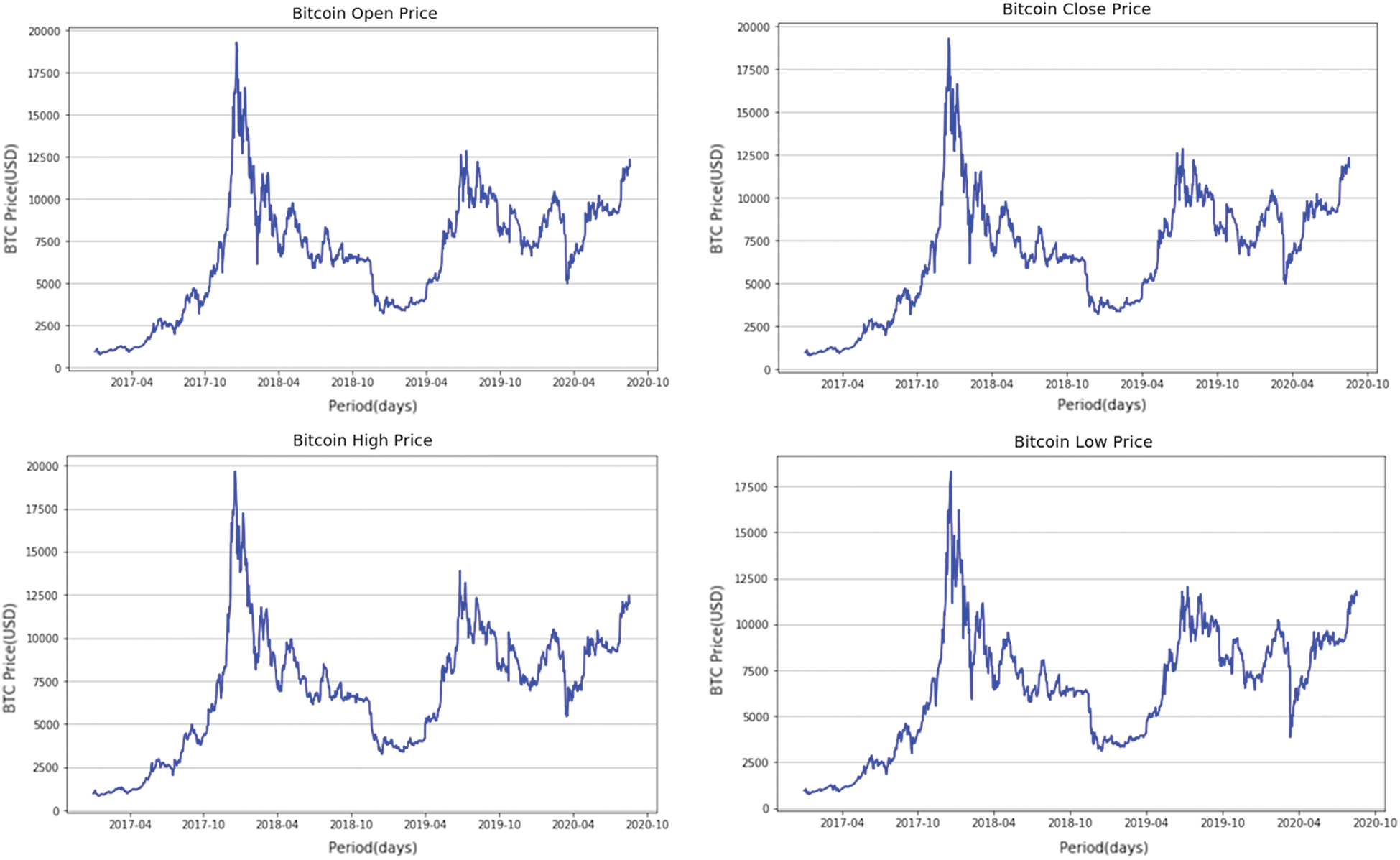
Figure 3: Bitcoin candlestick prices (OHLC) overtime. The figures emphasize that the price of the Bitcoin candlestick is volatile in all features. OHLC, open, high, low, and close
Recurrent neural networks (RNNs) are suitable for time series modeling. However, RNNs suffer from a problem known as vanishing gradient. The most common variants of RNN that solved that problem are long short-term memory (LSTM) and gated recurrent unit (GRU), selected in this work to predict the Bitcoin candlesticks. Besides, these two models are efficient at remembering long-term dependencies.
3.3.1 The Theoretical Basis of the Models
In the following discussion, the theoretical bases of the LSTM and GRU models are explained. LSTM was first introduced by Hochreiter et al. [20] as an extension of RNN. It is designed to solve the vanishing gradient problem and works tremendously well on time-series with long-term information problems. Currently, LSTM is widely utilized in stock price prediction and natural language processing. The internal structure of the LSTM model is shown in Fig. 4.
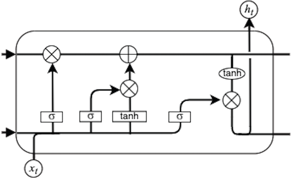
Figure 4: Long short term memory (LSTM) internal representation. LSTM contains three gates: input, forget, and output
The cell state and hidden state are utilized to collect and send data to the next state. To define if the data can pass through or not, input, output, and forget gates are utilized, all of which depend on data priority. Thus, the vanishing gradient problem can be solved, as described in Eqs. (2)–(6).
where Xt is the input, i is the input gate, f is the forget gate, o is the output gate, c is the cell state, h is the hidden state,
GRU was developed based on LSTM with a less complicated structure by tuning the gate in the LSTM to reset and update the gate. The reset gate is used to limit the amount of back-state data used with the current input data, while the update gate is intended to determine the amount of back-state data collection. Fig. 5 shows the structure of GRU nodes.
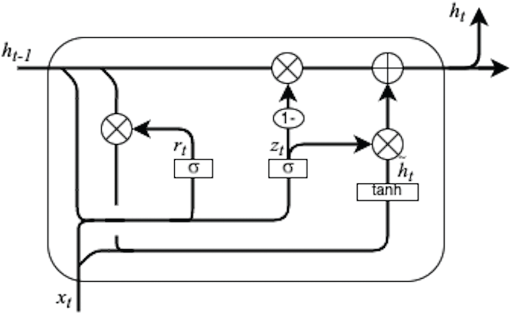
Figure 5: Gated recurrent unit (GRU) internal representation. GRU contains two gates: reset and update
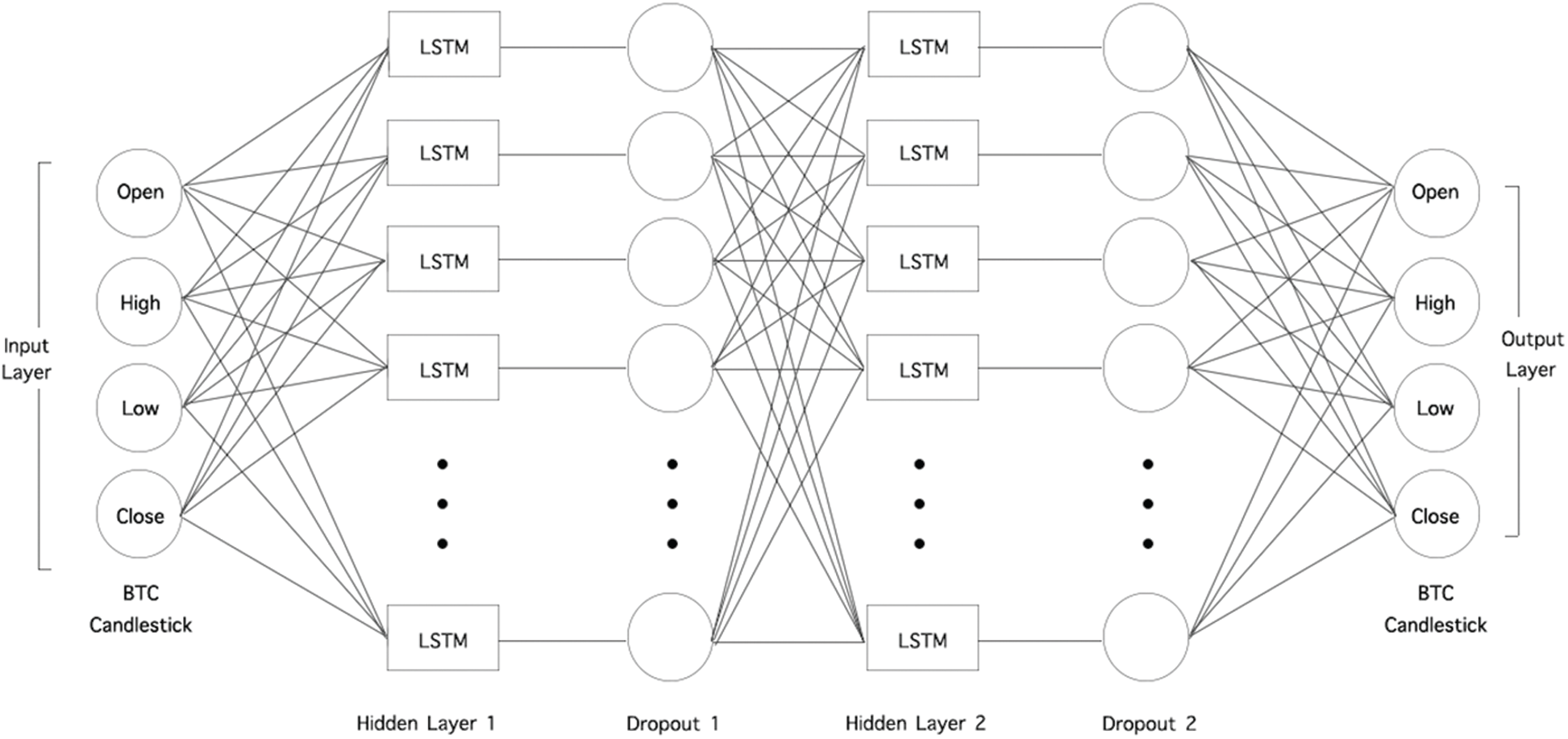
Figure 6: The structure of the long short term memory (LSTM) model
Figs. 6 and 7 show the LSTM and GRU structure employed to develop the prediction model. As shown in the figures, there is an input layer, two hidden layers, and one output layer. The input layer contains the Bitcoin candlestick, which involves the four features: the opening price, highest price, lowest price, and closing price (OHLC). The output layer contains the Bitcoin candlestick. We used two hidden layers. Each of the hidden layers has a regularization function, which was added to reduce overfitting. The regularization function used is dropout, which drops a random unit of the model. The use of two hidden layers is motivated by Velankar et al. [13], and the use of the dropout function is inspired by Yogeshwaran et al. [14]. To optimize weight, we use an Adam optimizer, which was also used by Yogeshwaran et al.
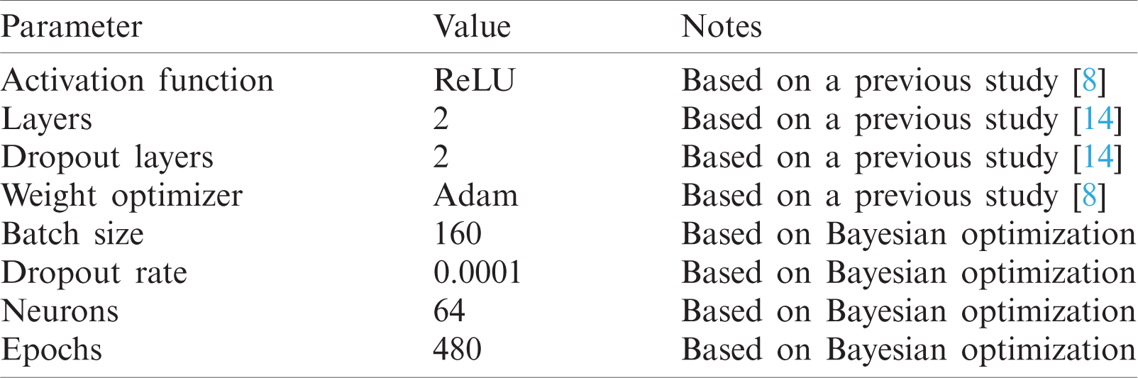
All the parameters mentioned above, i.e., Layers, Dropout layers, Weight optimizer, and Activation function, were configured based on previous studies. However, for other parameters needed to complete the model’s structure, i.e., Batch size, Dropout rate, Neurons, and Epochs, we had to find a proper way to choose their values. Based on multiple attempts at identifying the parameter values, we found that the babysitting approach (also known as trial and error) is not suitable. It is cumbersome and time-consuming because it is based on guessing. Thus, we utilized the Bayesian optimization technique to optimize the missing values alongside known values. Bayesian optimization is a method that uses an approximation to find the global optimum in a minimum number of steps without the need for guessing. Based on Bayesian optimization, the values of Batch size, Dropout rate, Neurons, and Epochs were identified as 160, 0.0001, 64, and 480, respectively. The complete list of the parameters’ configurations utilized in the prediction model is presented in Tab. 4.
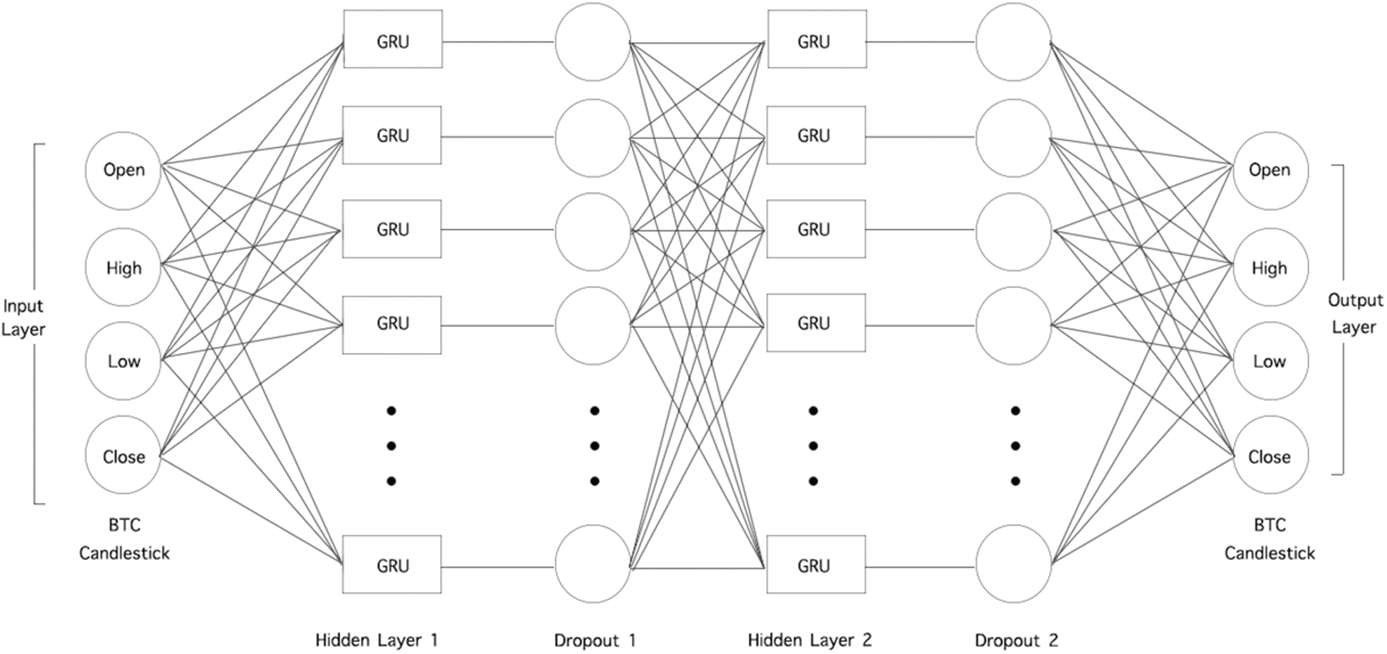
Figure 7: The structure of the gated recurrent units (GRU) model
Table 4: LSTM and GRU models’ parameter configurations
The train/test split is the applied method in the training and testing phases, where 80% of the records were utilized for training, and the remaining 20% was used for testing. The model was executed in the Python programming language, including several libraries such as Keras, Scikit-learn, Requests, NumPy, and Pandas. The Keras and the Scikit-learn libraries were used to build the model. The Requests library was used to call the API to get the real-time dataset. For data pre-processing, NumPy and Pandas were utilized. To accelerate the training time, the Colab graphics processing unit (GPU) was used. Using the GPU, it takes 49 min to train the 7984 records in 4-h intervals compared to 379 min when using the traditional CPU.
To measure the performance of the real-time prediction model, five metrics are used: mean absolute percentage error (MAPE), root mean square error (RMSE), MSE, mean absolute error (MAE), and R2. The MAPE is defined as the mean or average of the absolute percentage errors of forecasts. Error is defined as actual or observed value minus the forecasted value. The MAPE metric is expressed, as shown in Eq. (7).
The MSE is defined as the average of the squared error used as the loss function for least-squares regression and expressed in Eq. (8).
The RMSE measures the average magnitude of the errors in a set of predictions without recognizing their direction. This is the same as MSE, but the value’s root is considered while determining the model’s accuracy. The corresponding equation is shown below.
The MAE measures the average magnitude of the errors in a set of forecasts without considering their direction. It measures accuracy for continuous variables. The MAE metric is denoted, as shown in Eq. (10).
The R2 coefficient is described as the variance ratio in the dependent variable predictable from the independent variable(s) and expressed in Eq. (11).
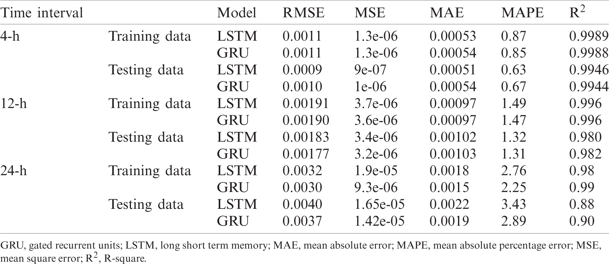
The LSTM and GRU prediction models were applied to 4, 12, and 24 h real-time Bitcoin data for three years, i.e., from January 1, 2017 to August 27, 2020, using the selected features explained earlier in Section 3. To measure the models’ performance, we used the measures mentioned in Section 3.4 to train and test data. Tab. 5 shows the LSTM and GRU models’ prediction results with the three intervals: 4, 12, and 24 h.
As shown in Tab. 5, the LSTM model outperformed the GRU with the 4-hour interval in all the performance measures. Specifically, it achieved an RMSE of 0.0009, an MSE of 9e-07, an MAE of 0.00051, and MAPE of 0.63, and an R2 of 0.9946. On the other hand, with the 12-h interval, the GRU model outperformed the LSTM model in all performance measures except the MAE measure. Specifically, the performance measures were as follows: RMSE was 0.00177, MSE was 3.2e-06, MAE was 0.00102, MAPE was 1.31, and R2 was 0.982. Like the 12-h interval results, the GRU model also outperformed the LSTM model with the 24-h interval, but in all measures. The performance measures were as follows: RMSE was 0.0037, MSE was 1.42e-05, MAE was 0.0019, MAPE was 2.89, and R2 was 0.90.
Table 5: Prediction performance of the with LSTM & GRU based on three time intervals
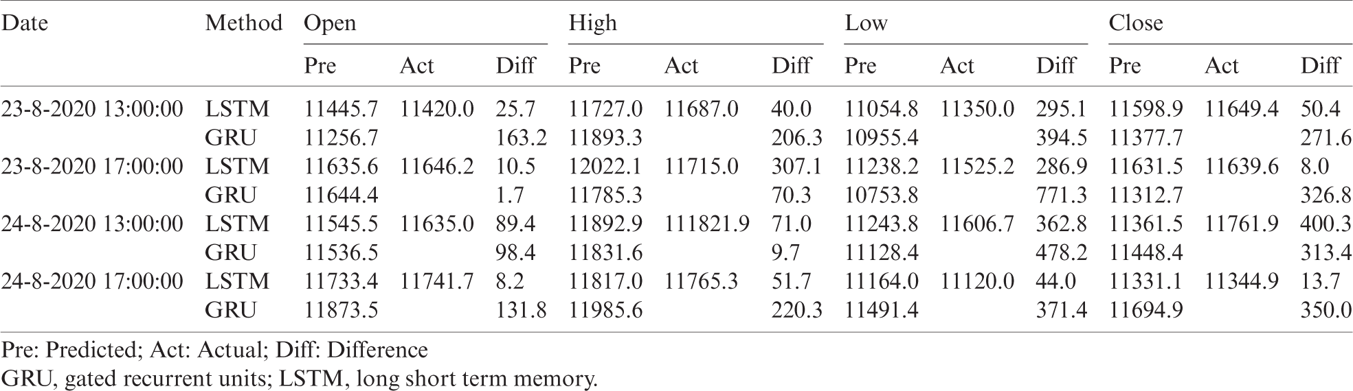
To get an overview of the LSTM and GRM models’ prediction results, the predicted Bitcoin daily close is shown graphically in Fig. 8 for the 4, 12, 24-h interval, respectively. In the figure, the predicted value of the daily close is compared with the actual value where the x-axis represents the date, and the y-axis represents the corresponding Bitcoin close price in U.S. dollars. As shown in Fig. 8, the lines representing the actual and predicted values are very close. To better compare between the two models, Fig. 9 zooms in and shows the predicted values of daily close for only three days. This is applied for each of the three intervals: the 4, 12, and 24 h. These results confirmed the results that we have shown earlier in Tab. 5, where the LSTM model outperformed GRU with the 4-h interval, and GRU outperformed the LSTM model for the other two intervals. However, the best-performing model is the LSTM model. For more detailed results for all models, Tabs. 6–8 presents four samples of the predicted and actual values of the Bitcoin candlesticks for the LSTM and the GRU model with all intervals. Specifically, the tables present the predicted values of the Bitcoin open, high, low, and close and how far they are from the actual values.
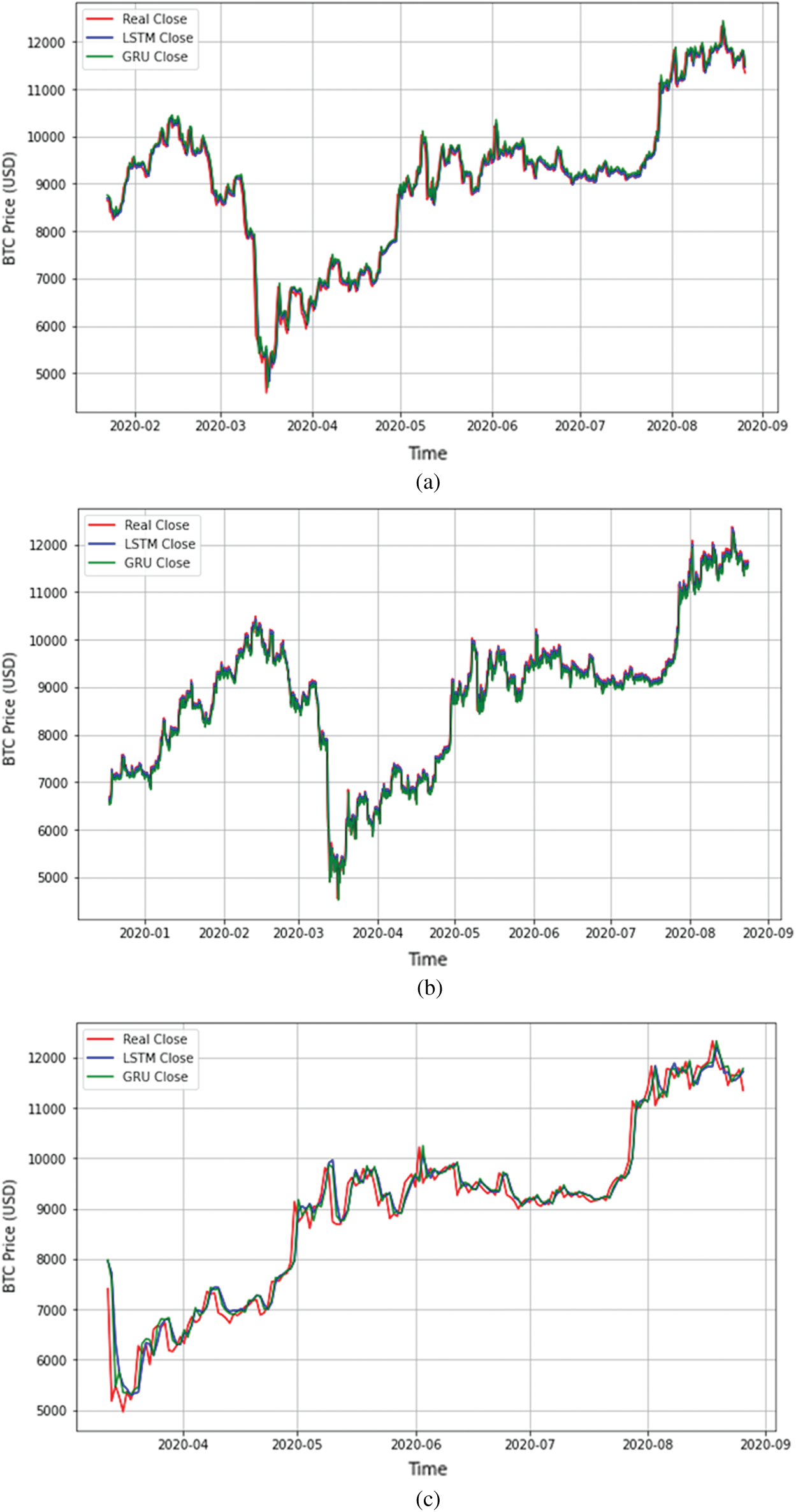
Figure 8: Overall prediction of Bitcoin close price based on LSTM and GRU with all intervals. (a) For 4-h interval, (b) For 12-h interval, and (c) For a 24-h interval
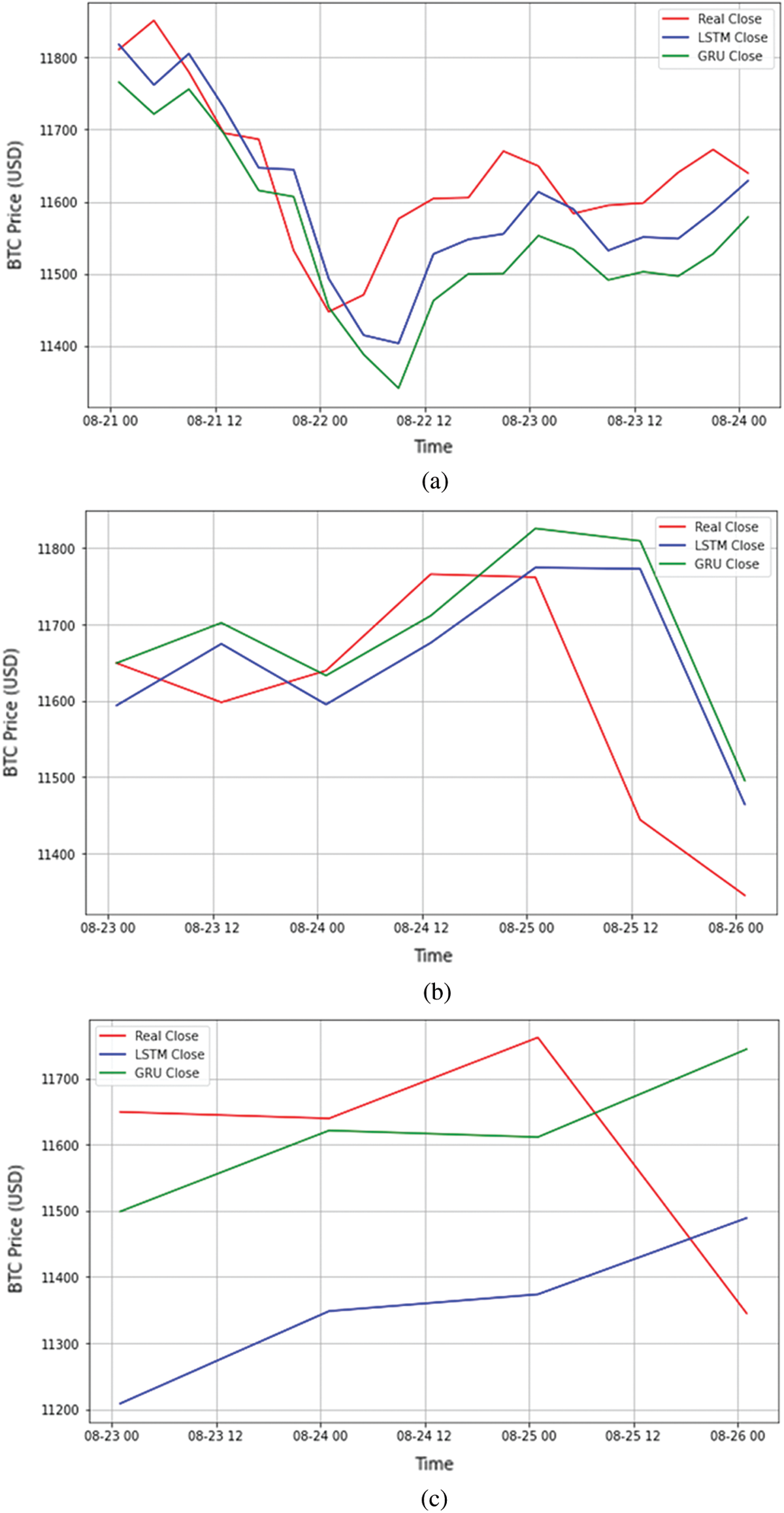
Figure 9: Sample Prediction of Bitcoin close price of three days: (a) For a 4-h interval, (b) for 12-h interval. and (c) for a 24-h interval
Table 6: Sample prediction of the Bitcoin candlestick for the next 4-h
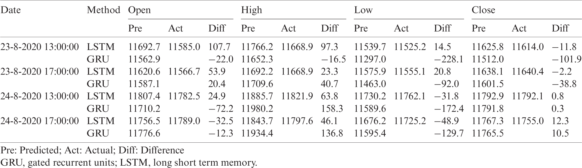
Table 7: Sample prediction of the Bitcoin candlestick for the next 12-h
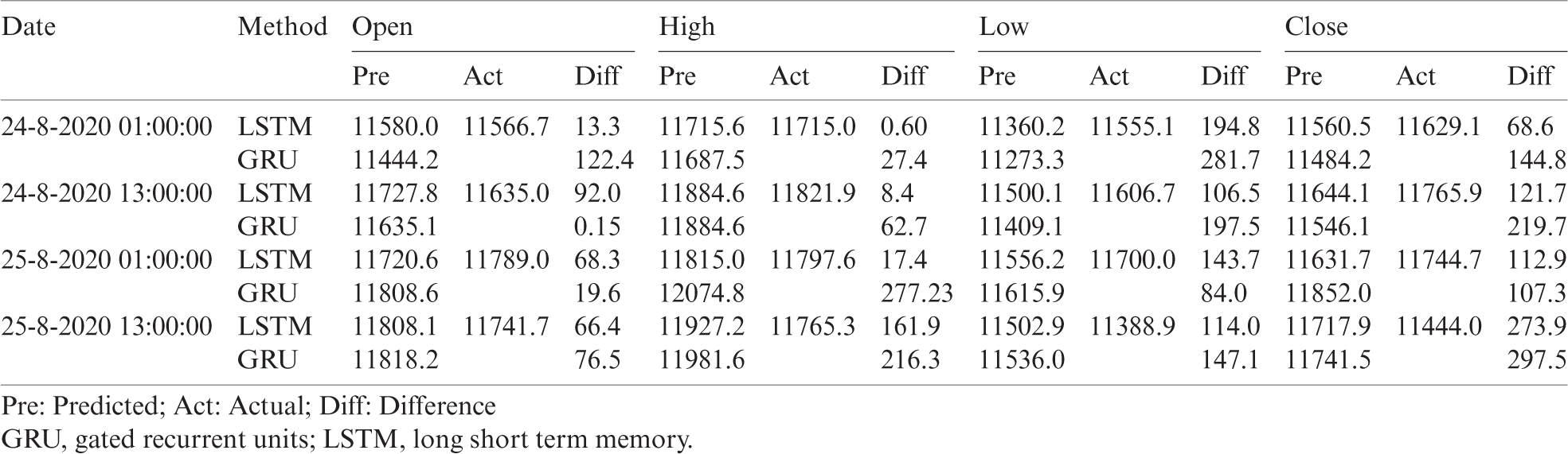
Table 8: Sample prediction of the Bitcoin candlestick for the next 24-h
Based on the results presented earlier, we can derive the following findings:
1. The LSTM model outperformed the GRU with the 4-h interval in all the performance measures. The GRU model gives some prediction readings that are slightly far from the actual prices. Based on the results presented in Tab. 6, the highest difference values between the predicted price and the actual price was produced by the GRU model, i.e., 158.3, −228.1, −101.9 for the high, low, and close prices, respectively.
2. The GRU model outperformed the LSTM model for the other two intervals. However, the best-performed model was the LSTM model with the 4-h interval. This model achieved the best performance, i.e., the lowest values of RMSE, MSE, MAE, and MAPE, and the highest value of R2.
The performance of the prediction model proposed in this study is evaluated and compared with previous models in the following section.
The results are evaluated in two ways. First, the best-performing model is compared with itself if it applied for historical data without the live (i.e., real-time) data. Second, the best-performing models in each interval are compared with similar models of previous studies.
5.1 Self-Comparison: Historical vs. Real-Time
For evaluation, we test the best performance prediction model (LSTM with 4-h interval) once with a Bitcoin historical dataset (Fig. 10), and again with both real-time Bitcoin data and historical data (Fig. 11). As shown in the figures, the real-time based model performed better than the historical-based model. This is obvious from the closeness of the two lines representing the actual and predicted values of Bitcoin daily close.
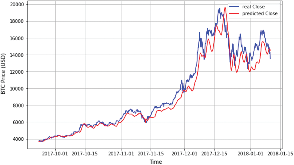
Figure 10: Predictions of the best-performed model (LSTM with 4-h interval) using historical data. Real-time based model performed better. LSTM, long short term memory
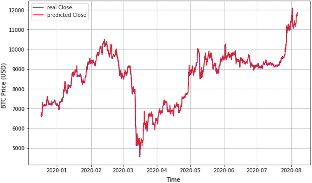
Figure 11: Predictions of the best-performed model (LSTM with 4-h interval) using real-time data. The close predicted prices are not far from the actual prices. LSTM, long short term memory
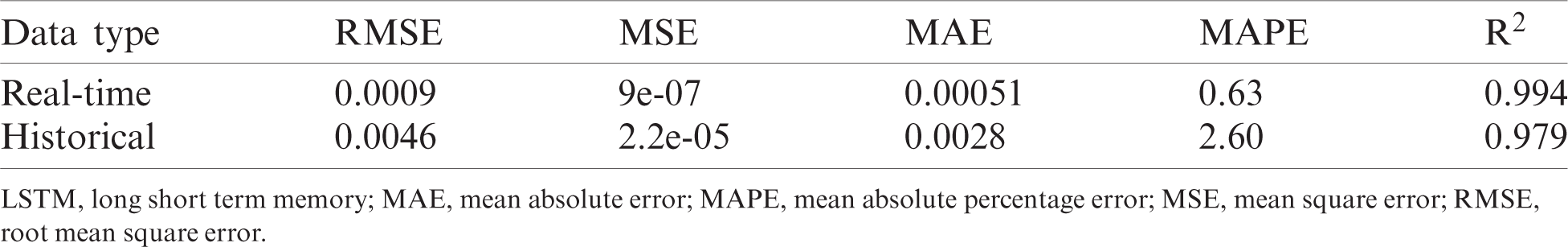
To get a better idea about the two models’ performance, Tab. 9 shows both models’ performance metrics that use LSTM with 4 h. As shown in the table, the real-time model outperformed the historical-based model in RMSE, MSE, MAE, MAPE, and R2.
Table 9: Performance of the 4-hour LSTM model with real-time data and historical data
5.2 A Comparison with the State-of-the-Art Models
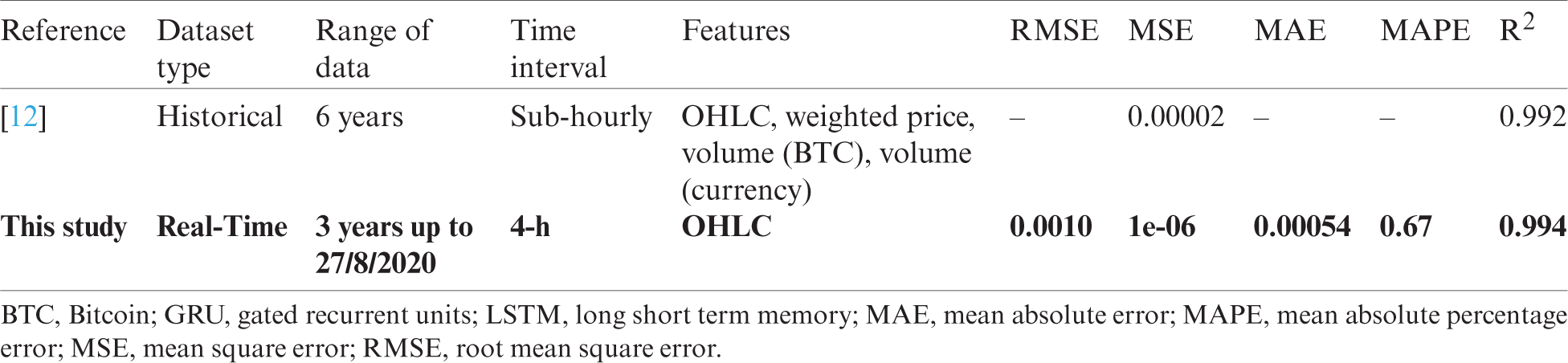
The model is compared with previous studies that have applied LSTM and GRU to predict Bitcoin price. The comparison is made in terms of performance metrics (see Tabs. 10 and 11). As shown in the tables, the proposed real-time model outperformed the state-of-the-art models in terms of RMSE, MSE, MAE, MAPE, and R2. This supports our assumption that including real-time data in addition to the historical data does improve prediction model performance.
Table 10: comparison of the LSTM real-time based model with previous studies that used LSTM
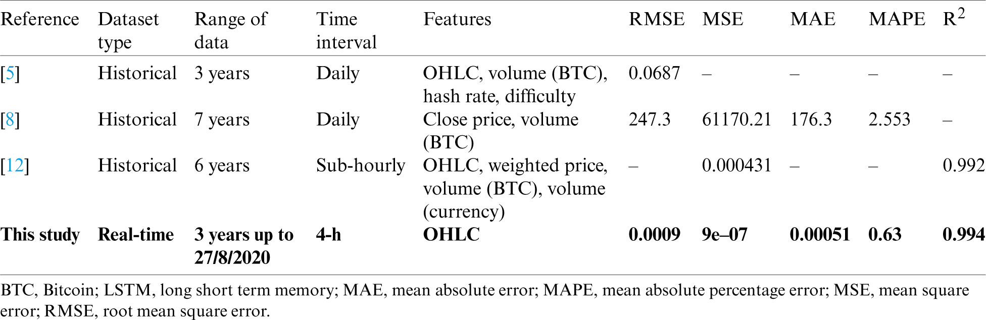
Table 11: comparison of the GRU real-time based model with previous studies that used GRU
The price of Bitcoin is considered to be very unpredictable. That is, within hours of a day, the price can go up and down. Consequently, potential users are averse to the risks inherent to Bitcoin. In deciding the buying and selling opportunities, an accurate forecast of the Bitcoin price would help alleviate risk. This study proposed using two deep learning algorithms, LSTM and GRU, for short-term real-time Bitcoin prediction models. The models were applied to three intervals (4, 12, and 24-h) based on Bitcoin real-time (i.e., live) data along with Bitcoin historical data. The LSTM model with a 4-h interval was the best-performing model and outperformed the state-of-the-art models, which were mainly based on historical data sets without taking real-time data into account. We believe that such a model can effectively lead to the learning of potential Bitcoin price trends and help people determine when to buy and sell Bitcoins. Among the conclusions made by this study is that Bayesian optimization is a promising approach to define the values of parameters and can be used by other researchers to construct high-performance prediction models in similar areas such as the stock market. Future works can include the extension of the real-time dataset to have more exchanges, e.g., Bitstamp in addition to Kraken exchange. Further efforts may include the construction of Bitcoin prediction models based on other machine and deep learning algorithms.
Acknowledgement: Researchers would like to thank the Deanship of Scientific Research, Qassim University for funding publication of this project.
Funding Statement: The authors received no specific funding for this study.
Conflicts of Interest: The authors declare that they have no conflicts of interest to report regarding the present study.
1. S. Abboushi, “Global virtual currency—Brief overview,” Journal of Applied Business and Economics, vol. 19, no. 6, pp. 10–18, 2017. [Google Scholar]
2. Y. Peng, P. H. M. Albuquerque, J. M. C. de Sá, A. J. A. Padula and M. R. Montenegro, “The best of two worlds: Forecasting high frequency volatility for cryptocurrencies and traditional currencies with support vector regression,” Expert Systems with Applications, vol. 97, no. 3, pp. 177–192, 2018. [Google Scholar]
3. A. Urquhart, “Price clustering in Bitcoin,” Economics Letters, vol. 159, no. 4, pp. 145–148, 2017. [Google Scholar]
4. S. Nakamoto, “Bitcoin: A peer-to-peer electronic cash system,” Technical Report, 2019. [Online]. Available: https://bitcoin.org/bitcoin.pdf. [Google Scholar]
5. S. McNally, J. Roche and S. Caton, “Predicting the price of Bitcoin using machine learning,” in Euromicro Int. Conf. on Parallel, Distributed and Network-based Processing, Cambridge, UK, pp. 339–343, 2018. [Google Scholar]
6. R. Albariqi and E. Winarko, “Prediction of Bitcoin price change using neural networks,” in Int. Conf. on Smart Technology and Applications, Surabaya, Indonesia, pp. 1–4, 2020. [Google Scholar]
7. M. Van Alstyne, “Why Bitcoin has value,” Communications of the ACM, vol. 57, no. 5, pp. 30–32, 2014. [Google Scholar]
8. T. Shintate and L. Pichl, “Trend prediction classification for high frequency Bitcoin time series with deep learning,” Journal of Risk and Financial Management, vol. 12, no. 1, pp. 17, 2019. [Google Scholar]
9. S. C. Purbarani and W. Jatmiko, “Performance comparison of Bitcoin prediction in big data environment,” in Int. Workshop on Big Data and Information Security, Jakarta, pp. 99–106, 2018. [Google Scholar]
10. I. Madan, S. Saluja and A. Zhao, “Automated Bitcoin trading via machine learning algorithms,” 2015. [Online]. Available: http://cs229.stanford.edu/proj2014/Isaac%20Madan,%20Shaurya%20Saluja,%20Aojia%20Zhao,Automated%20Bitcoin%20Trading%20via%20Machine%20Learning%20Algorithms.pdf. [Google Scholar]
11. C. Wu, C. Lu, Y. Ma and R. S. Lu, “A new forecasting framework for Bitcoin price with LSTM,” in IEEE Int. Conf. on Data Mining Workshops, Singapore, pp. 168–175, 2018. [Google Scholar]
12. T. Phaladisailoed and T. Numnonda, “Machine learning models comparison for Bitcoin price prediction,” in Int. Conf. on Information Technology and Electrical Engineering, Kuta, Indonesia, pp. 506–511, 2018. [Google Scholar]
13. S. Velankar, S. Valecha and S. Maji, “Bitcoin price prediction using machine learning,” in Int. Conf. on Advanced Communication Technology, Korea, pp. 144–147, 2018. [Google Scholar]
14. S. Yogeshwaran, M. J. Kaur and P. Maheshwari, “Project based learning: Predicting Bitcoin prices using deep learning,” in IEEE Global Engineering Education Conf., Dubai, United Arab Emirates, pp. 1449–1454, 2019. [Google Scholar]
15. G. Serafini, Y. Ping, Z. Qingquan, M. Brambilla, W. Jiayue et al., “Sentiment-driven price prediction of the Bitcoin based on statistical and deep learning approaches,” in IEEE Int. Joint Conf. on Neural Networks, Glasgow, United Kingdom, pp. 1–8, 2020. [Google Scholar]
16. M. Rizwan, S. Narejo and M. Javed, “Bitcoin price prediction using deep learning algorithm,” in IEEE Int. Conf. on Mathematics, Actuarial Science, Computer Science and Statistics, Karachi, Pakistan, pp. 1–7, 2019. [Google Scholar]
17. S. Roy, S. Nanjiba and A. Chakrabarty, “Bitcoin price forecasting using time series analysis,” in IEEE Int. Conf. of Computer and Information Technology, Dhaka, Bangladesh, pp. 1–5, 2018. [Google Scholar]
18. P. Linardatos and S. Kotsiantis, “Bitcoin price prediction combining data and text mining, smart innovation,” Systems and Technologies, vol. 170, pp. 49–63, 2020. [Google Scholar]
19. D. C. Mallqui and R. A. Fernandes, “Predicting the direction, maximum, minimum and closing prices of daily Bitcoin exchange rate using machine learning techniques,” Applied Soft Computing, vol. 75, no. 2, pp. 596–606, 2019. [Google Scholar]
20. S. Hochreiter and J. Schmidhuber, “Long short-term memory,” Neural Computation, vol. 9, no. 8, pp. 1735–1780, 1997. [Google Scholar]
 | This work is licensed under a Creative Commons Attribution 4.0 International License, which permits unrestricted use, distribution, and reproduction in any medium, provided the original work is properly cited. |