DOI:10.32604/cmc.2021.016626
| Computers, Materials & Continua DOI:10.32604/cmc.2021.016626 | |
| Article |
An Optimal Big Data Analytics with Concept Drift Detection on High-Dimensional Streaming Data
1Department of Mathematics, Faculty of Science, New Valley University, El-Kharga, 72511, Egypt
2Department of Information Systems, College of Computer and Information Sciences, Princess Nourah Bint Abdulrahman University, Riyadh, 84428, Saudi Arabia
3Department of Computer Sciences, College of Computer and Information Sciences, Princess Nourah Bint Abdulrahman University, Riyadh, 84428, Saudi Arabia
4Department of Entrepreneurship and Logistics, Plekhanov Russian University of Economics, Moscow, 117997, Russia
5Department of Logistics, State University of Management, Moscow, 109542, Russia
*Corresponding Author: Romany F. Mansour. Email: romanyf@scinv.au.edu.eg
Received: 07 January 2021; Accepted: 01 March 2021
Abstract: Big data streams started becoming ubiquitous in recent years, thanks to rapid generation of massive volumes of data by different applications. It is challenging to apply existing data mining tools and techniques directly in these big data streams. At the same time, streaming data from several applications results in two major problems such as class imbalance and concept drift. The current research paper presents a new Multi-Objective Metaheuristic Optimization-based Big Data Analytics with Concept Drift Detection (MOMBD-CDD) method on High-Dimensional Streaming Data. The presented MOMBD-CDD model has different operational stages such as pre-processing, CDD, and classification. MOMBD-CDD model overcomes class imbalance problem by Synthetic Minority Over-sampling Technique (SMOTE). In order to determine the oversampling rates and neighboring point values of SMOTE, Glowworm Swarm Optimization (GSO) algorithm is employed. Besides, Statistical Test of Equal Proportions (STEPD), a CDD technique is also utilized. Finally, Bidirectional Long Short-Term Memory (Bi-LSTM) model is applied for classification. In order to improve classification performance and to compute the optimum parameters for Bi-LSTM model, GSO-based hyperparameter tuning process is carried out. The performance of the presented model was evaluated using high dimensional benchmark streaming datasets namely intrusion detection (NSL KDDCup) dataset and ECUE spam dataset. An extensive experimental validation process confirmed the effective outcome of MOMBD-CDD model. The proposed model attained high accuracy of 97.45% and 94.23% on the applied KDDCup99 Dataset and ECUE Spam datasets respectively.
Keywords: Streaming data; concept drift; classification model; deep learning; class imbalance data
The progressive deployment of Information Technology (IT) in different domains results in the production of huge volumes of data. The maximum velocity of big data outperforms the computational approach followed by classic models. Some of the examples are Sensor Networks (SN), spam filtering mechanism, traffic management, and Intrusion Detection System (IDS). In general, data-stream S is highly unbounded, while the regular sequence of samples arrives frequently in a robust manner. However, this framework has a primary limitation i.e., the presence of concept drift issues and the principle behind this model is drifted in dynamic fashion. This issue must be resolved. Concept drift is a common problem that exists in real-time practical applications. For example, in recommended systems, the choice of a user may vary and it tend to change frequently based on situation, finance, climatic conditions, and other such factors. These changes may reduce the classification function. Basically, a classifier should be capable of realizing these changes and react to them appropriately. Followed by, learning models are developed to handle static platforms. But real-time applications have dynamic hierarchy. Here, concept drift is reported as non-stationary platform in which the target concept is modified in the presence of controversial training and application data [1]. Different domains have concept drift-based issues such as monitoring, management and strategic planning, personal guidance, and so on. The current research work makes use of technologies to handle and predict the concept drift.
Preprocessing is an important task since the storage space is minimum and the samples need to be scanned in single pass. Further, collective samples should be decided from data stream as well. The main purpose of sampling is to select a part of data stream and regard it as ‘entire system.’ When computing stream data, irregular data phenomenon is important since it is utilized in several applications like weather data forecasting, anomalous prediction, social media mining, etc. Next, class imbalance is feasible when representing a single instance or if the values are more than others. Classes, with maximum number of data samples, are named as majority classes. While the remaining classes are referred to as minority classes. In stream data classification, the majority class overcomes the samples and eliminates the minority class.
Pre-processing is a better solution to balance the distribution of class. When the reservoir size is unnecessarily allocated for stream data sourced from different devices, it increases the imbalance problem. So, resampling is applied extensively to manage the sample set through instant elimination of majority class and the process is called under-sampling and oversampling. But, the sensitivity of learning accuracy, in class imbalance, is based on the distribution of minority classes and degree of overlap among the classes. Concept drift denotes the modifications in distributed samples due to major problems in stream data examination.
This research work presents a new Multi-Objective Metaheuristic Optimization-based Big Data Analytics with Concept Drift Detection (MOMBD-CDD) on High-Dimensional Streaming Data. The presented MOMBD-CDD model handles class imbalance problem using a Synthetic Minority Over-sampling Technique (SMOTE). To determine oversampling rate and the neighboring points of SMOTE, Glowworm Swarm Optimization (GSO) algorithm is employed. Further, Statistical Test of Equal Proportions (STEPD), a CDD technique is utilized. At last, bidirectional Long Short-Term Memory (Bi-LSTM) model is applied for classification. To enhance the classifier results of Bi-LSTM model, GSO-based hyperparameter tuning process is performed. The proposed MOMBD-CDD model was evaluated through comprehensive analysis of high dimensional benchmark streaming datasets namely intrusion detection (NSL KDDCup) dataset and ECUE dataset.
Barros et al. [2] presented Reactive Drift Detection Method (RDDM) based on DDM. This technique eliminates the previous samples of prolonged models. It helps in predicting drifts as well as increasing the accuracy. Li et al. [3] projected Ensemble Decision Trees for Concept (EDTC) drift data streams by mimicking cut-points in tree development. The method was used along with three diverse random Feature Selection (FS) models. After reaching an instance, a growing node randomly divides the features and eliminates the unwanted branches. In this research, EDTC applies two thresholds and local data distributions are employed to predict the drift. Ross et al. [4] proposed Exponentially Weighted Moving Average (EWMA) for Concept DD (ECDD), a drift detection model depending on exponentially-weighted average chart. The model used classification error stream and the developers required no data to be saved in storage space.
Widmer et al. [5] developed Floating Rough Approximation (FLORA) approach to handle CD with collective descriptors. In this study, variable-sized sample window was used for selecting the descriptors. Liu et al. [6] projected a DD in SN-relied Angle Optimized Global Embedding (AOGE) as well as Principal Component Analysis (PCA) method. PCA and AOGE intend to examine the projection difference and projection angle which are again applied in the prediction of drift. Bifet et al. [7] implied Adaptive Windowing (ADWIN2) mechanism, an extended version of ADWIN model. ADWIN2 has windows of different sizes which gets developed or reduced, when a concept drift is predicted. Additionally, supervised models are used in predicting the drifts under the application of elements present in a window. Xu et al. [8] deployed Dynamic Extreme Learning Machine (DELM) technology by leveraging Extreme Learning Machine (ELM) technique for drift prediction. The primary objective of this method was to apply a double hidden layer to train the network and enhance its performance.
Lobo et al. [9] established a popular Spiking Neural Network (NN) model in web learning data streams. This method primarily focused on the mitigation of size of neurons. By exploiting data limitation methods, the study reaped the benefits of compressed neuron learning potential. Zhang et al. [10] implied a 3-layered drift prediction model in text data stream. In this model, a layer represents multiple components such as label space, layer of feature space, and finally the layer of mapping labels as well as its features. Lobo et al. [11] illustrated DRED relied on multi-objective optimization for data labeling. The developers, in this paper, projected the significance of applying ensembles which possess the capability to deal with modifications in a data stream after its prediction.
Mirza et al. [12] proposed Ensemble of Subset Online Sequential Extreme Learning Machine (ESOS-ELM), a drift detection mechanism to solve the class imbalance issues. Arabmakki et al. [13] deployed Reduced labeled Samples Self Organizing Map (RLS-SOM) to overcome the issues in imbalanced data stream. The ensemble is used to classify Dynamic Weighted Majority (DWM) as per the new method under the application of labeled samples, if the drifts are selected. Lobo et al. [14] implied a possible mechanism to overcome the problems in imbalanced data streams. Next, the researchers have recommended the identification of essential samples from senior learners.
Sethi et al. [15] introduced MD3 (Margin Density DD) to predict the drift in unlabeled stream. When there is a deviation in margin density, a classifier has a collection of labeled samples that can be retrained. De Andrade Silva et al. [16] projected Fast Evolutionary Algorithm for Clustering (FEAC-data Streams) algorithm based on k-means clustering with k-automatic estimation of stream value. In this study, FEAC-Stream applied Page-Hinkley test to predict the reduction in quality of clusters to initialize k evolutionary models.
3 The Proposed MOMBD-CDD Model
Fig. 1 shows the workflow of the presented MOMBD-CDD model in big data environment. As illustrated, the online streaming of big data is initially preprocessed through three distinct ways such as conversion into .csv format, conversion of categorical to numerical data, and chunk generation. Next, the preprocessed data undergoes class imbalance handling process by following SMOTE-GSO algorithm. Followed by, the CDD process is performed as per STEPD technique. At last, Bi-LSTM model performs the classification while the model is already tuned by GSO algorithm to determine the hyperparameters.
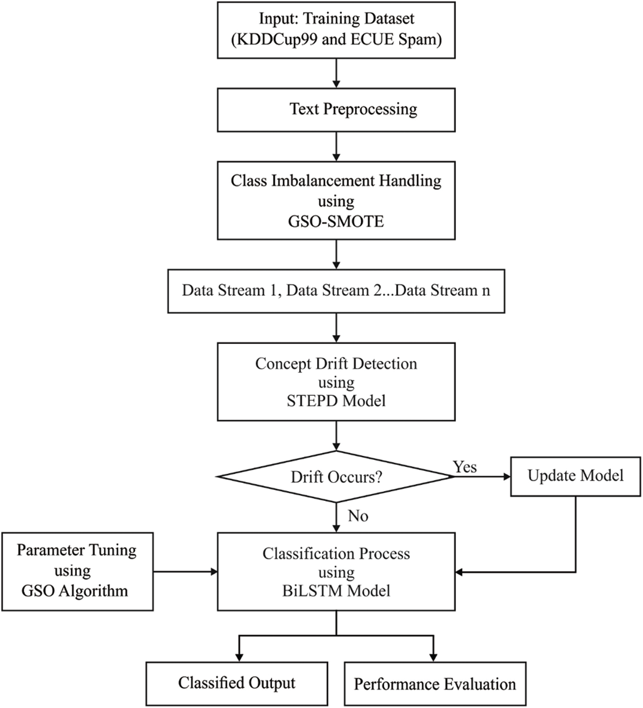
Figure 1: Working process of the proposed MOMBD-CDD model
CDD is considered as a major concern that needs to be resolved to predict a change-point in
Assume
The above-defined characteristic values from
To overcome the issues involved in big data streaming, Hadoop ecosystem and its corresponding elements are extensively applied. In distributed platform, Hadoop belongs to open source structure that allows its shareholders to save and compute big data functions through computer clusters using simple programming methods. With the help of maximum number of nodes from single server, both scalability and fault tolerance can be increased through this technique. Hadoop has three major components namely, MapReduce, Hadoop Distributed File System (HDFS), and Hadoop YARN. Based on Google File System (GFS), HDFS has been developed. It is regarded as a model that functions as per master/slave mechanism; when the master is comprised of numerous data nodes, it is referred to as original data and diverse name node is referred to as metadata. Hadoop Map Reduce is applied to generate drastic scalability over massive Hadoop clusters. This is also named as computational approach at Apache Hadoop core. Map Reduce is utilized to compute numerous data over large-scale clusters. There are two essential phases present in Map Reduce namely, Reduce and Map. Each phase is composed of pairs-like key values called input and output. Both output as well as input are secured, especially in file system. It is responsible for task scheduling, management, and re-implementation of the failed task. The infrastructure of Map Reduce contains a slave node manager and master resource manager for every cluster node.
Hadoop YARN is a model applied for cluster management. Based on the experience gained during primary Hadoop production, the above-mentioned model is labeled as 2nd generation Hadoop and is treated as a major attribute. Among Hadoop clusters, security, scalability, and data governance machines are some of the major aspects to be resolved while YARN serves as a main framework as well as a resource manager. To handle big data, alternate devices and elements are deployed over Hadoop infrastructure. Map Reduce method, a scheme of MRODC approach, is utilized in enhancing the classification scalability and robustness in computing. The following aspects are composed of MRODC method.
• Based on N-gram, Polarity score is checked for each sentence
• Based on Polarity score, data classification is performed
• Based on the classified data, new words and Term Frequency (TF) are evaluated
When applying diverse Data Mining (DM) models, the basic data from HDFS undergoes pre-processing. Using Map function, the iterations are processed simultaneously and are named as combiner function and reduce function respectively. The performance is measured when the Map approves every line from the sentence, as different pairs of key-value, since this is the input for Map function. Based on the developed corpus, Map function measures a data object value. Based on different grams, the value is determined. The result of a mapping function is forwarded to Combiner function. The whole set of data objects are retrieved from Combiner function after which the data is classified according to identical class. Consequently, it unifies the whole set of data with identical class values, and saves the sample values for Reducer function. The simulation result of a cluster is transmitted. From different classes, Reduce function retrieves complete data which can otherwise be called as the simulation outcome of Combiner function. After the data from different class labels is summarized and evaluated, the final results are attained in JHDFS along with class labels and the next iteration is proceeded.
Once the streaming data is preprocessed, class imbalance handling process is executed. SMOTE is defined as over-sampling mechanism by Chawla et al. [18] and it is generally processed in feature space rather than data space. Here, the count of samples for minority class in actual data set is improved. This is accomplished by developing synthetic instances which pose as extensive decision regions for minority class. However, naive over-sampling and replacement results in specific minority class. Novel synthetic samples are developed by two variables namely, over-sampling rate (%) and count of the nearest neighbors (k).
• Evaluate the difference between feature vector in minority class and k nearest neighbors (kNN).
• Enhance the distance attained earlier by random values between 0 and 1.
• Include the value gained from former step which is used to regain the measure of new feature vector.
The novel feature vector is developed by as follows
where xn refers to a new synthetic sample, x0 denotes a feature vector in minority class, xoi depicts the ith selected NN of xO, and
• Step 1: Gain the majority vote among features by considering kNN for nominal feature value. When both are symmetric, the values are selected randomly
• Step 2: Allocate the accomplished value for new synthetic minority class instance
To determine the sample rate and neighboring points of SMOTE, GSO algorithm is used. GSO algorithm applies glowworms with glowing quantity named luciferin, or agents. At the beginning, the glowworms are considered as initial solutions which are randomly distributed in problem space. Then, it travels to highly-illuminated place by the sensor range. At last, the brighter ones are collected and is referred to as an optimal solution for the given problem. In GSO, there are three phases listed in the following literature [20]. Fig. 2 illustrates the flowchart of GSO model.
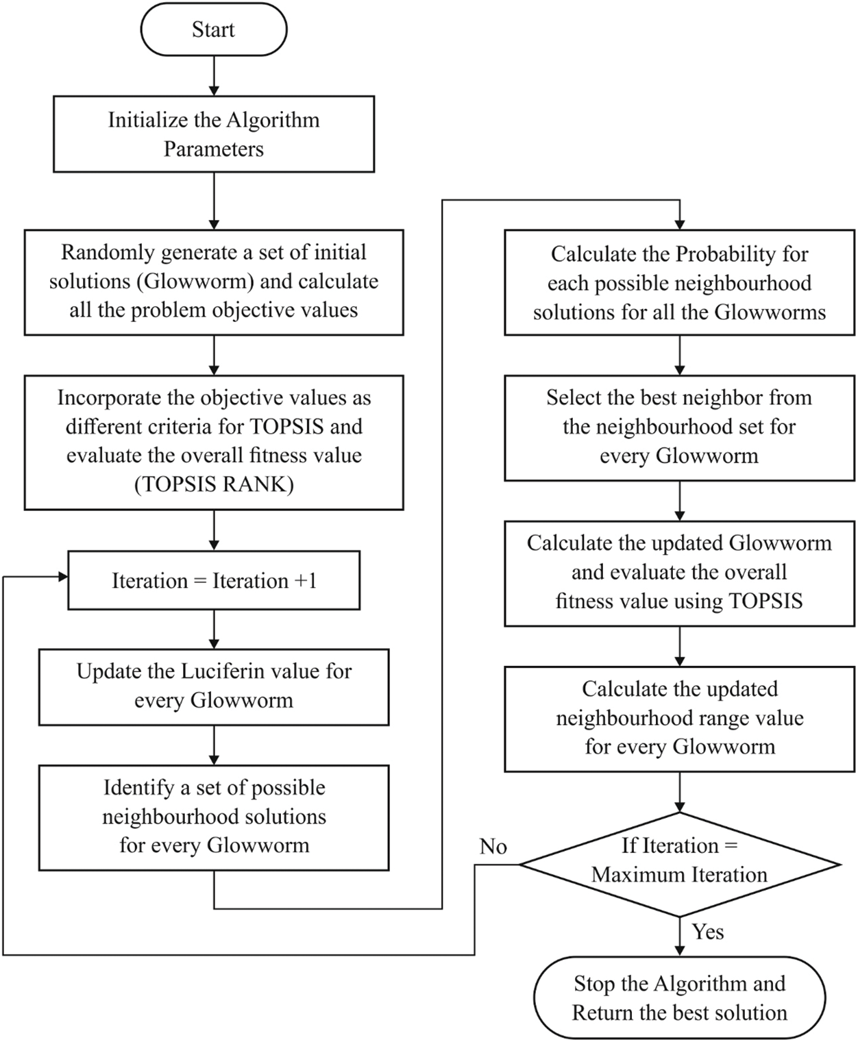
Figure 2: Flowchart of GSO model
The measure of luciferin glowworms is based on the objective function of recent position. The expression to upgrade the luciferin is given herewith.
where
where VPV means the overall voltage of PV cells in a series. The voltage of PV cell is projected as a function of present I. Hence, F denotes the performance of solar irradiation, current, and temperature. I signifies the variable to be optimized considering the position of glowworm, and S denotes the input parameter.
When an agent decides to move towards a supreme individual, it depends upon the probability mechanism. The probability of an agent i traveling to agent j is measured as given herewith.
where
where s denotes the step size and
3.3.3 Local-Decision Range Update Phase
Decision radius has to be upgraded on the basis of individuals in present range:
where
The model parameters are well operated in an extensive range of applications. While, only n and rs are referred to as parameters that influence the behavior of the model. The measures of high iteration value and glowworm number are applied, when GSO model is simulated.
STEPD observes the predictions of classifier to select signal warnings and drifts. It is composed of two parametrized thresholds which refer to important drift prediction levels as well as alerts i.e.,
In order to compare the accuracies of these two windows, STEPD defines a hypothesis test of similar proportions with frequent adjustment, as given in Eq. (1). Followed by, it is clear that r0 means the value of accurate predictions in n0 samples of previous window, rr defines the count of accurate predictions from
The final outcome of
Bi-LSTM model is employed at the end to determine the class label properly. Bi-LSTM is a hybrid mechanism, a resultant of combination of LSTM and Bi-directional Recurrent Networks (Bi-RNN). Recurrent Neural Network (RNN) is one of the well-known models evolved from Artificial Neural Networks (ANN) and is used to compute the sequences as well as time series. RNN is beneficial to encode the dependencies among inputs. Followed by, LSTM is developed to resolve the prolonged problems faced in RNN. LSTM is composed of few gates. In case of input layer, the input gate is available. While, for output layer, forget gate and output gate are present. Therefore, LSTM and RNN can be applied to acquire the data from existing content; thus, the output is further enhanced with the help of Bidirectional Bi-RNN. It is capable of handling two data from front end and backend. Fig. 3 shows the structure of Bi-LSTM model.
Thus, the benefits of LSTM in memory storage and Bi-RNN are applied in data accessing before and after Bi-LSTM. It makes Bi-LSTM to be benefitted for LSTM with feedback for consecutive layer [22]. Hence, Bi-LSTM with inputs of
where
where
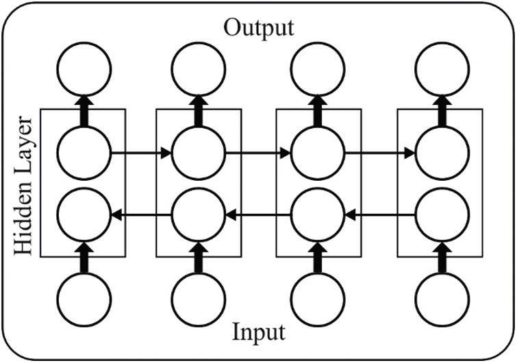
Figure 3: The structure of Bi-LSTM
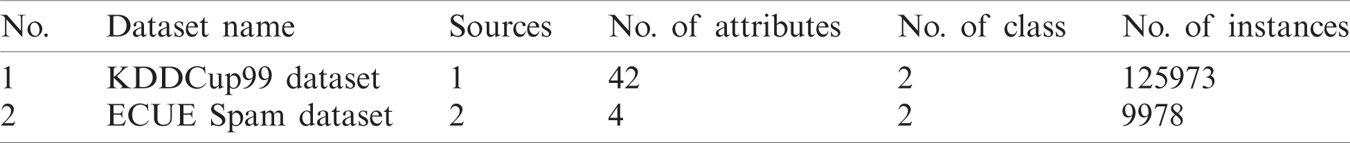
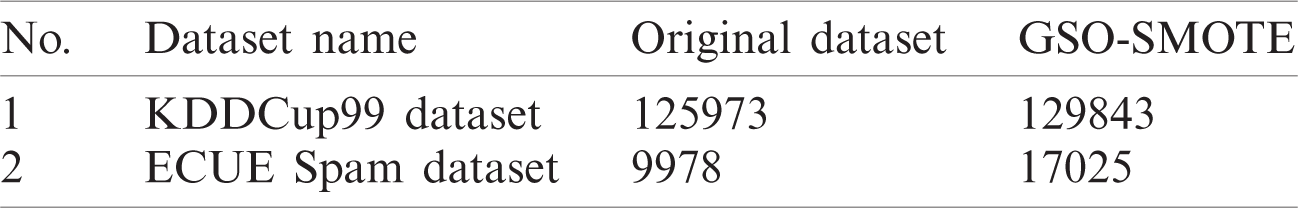
The performance of the presented MOMBD-CDD model was validated in this section using two datasets namely, KDDCup99 [23] and ECUE spam dataset [24]. Tab. 1 shows the information relevant to these datasets. Firstly, the KDDCup 99 dataset includes a set of 125973 instances with two class labels and 42 attributes. Secondly, the ECUE spam dataset comprises of 4 attributes with 9978 instances with two class labels.
Table 1: The dataset description
Tab. 2 shows the results attained after class imbalance handling process by GSO-SMOTE technique. The table reports that the GSO-SMOTE technique sampled the original KDDCup99 dataset with 125973 instances into 129843 instances. Besides, on the applied ECUE spam dataset, the GSO-SMOTE model sampled 17025 instances from the original 9978 instances.
Table 2: Results of the analysis of original dataset vs. GSO-SMOTE
Tab. 3 and Figs. 4–5 demonstrate the classification results of analysis for the presented MOMBD-CDD model upon applied KDDCup99 and ECUE spam datasets. The resultant values of the presented MOMBD-CDD model on applied KDDCup99 dataset accomplished a higher sensitivity, specificity, precision, accuracy, F-score, and kappa value of 97.84%, 95.43%, 97.17%, 97.45%, 96.51%, and 95.29% respectively. At the same time, the obtained experimental values denote that MOMBD-CDD model processed the ECUE spam dataset with maximum sensitivity, specificity, precision, accuracy, F-score, and kappa value of 94.88%, 93.20%, 94.19%, 94.23%, 93.56%, and 92.90% respectively.
Table 3: Result attained by the proposed models in terms of different measures
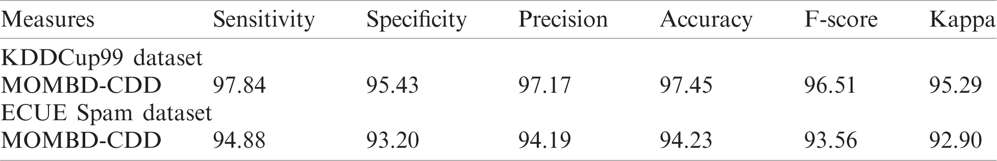
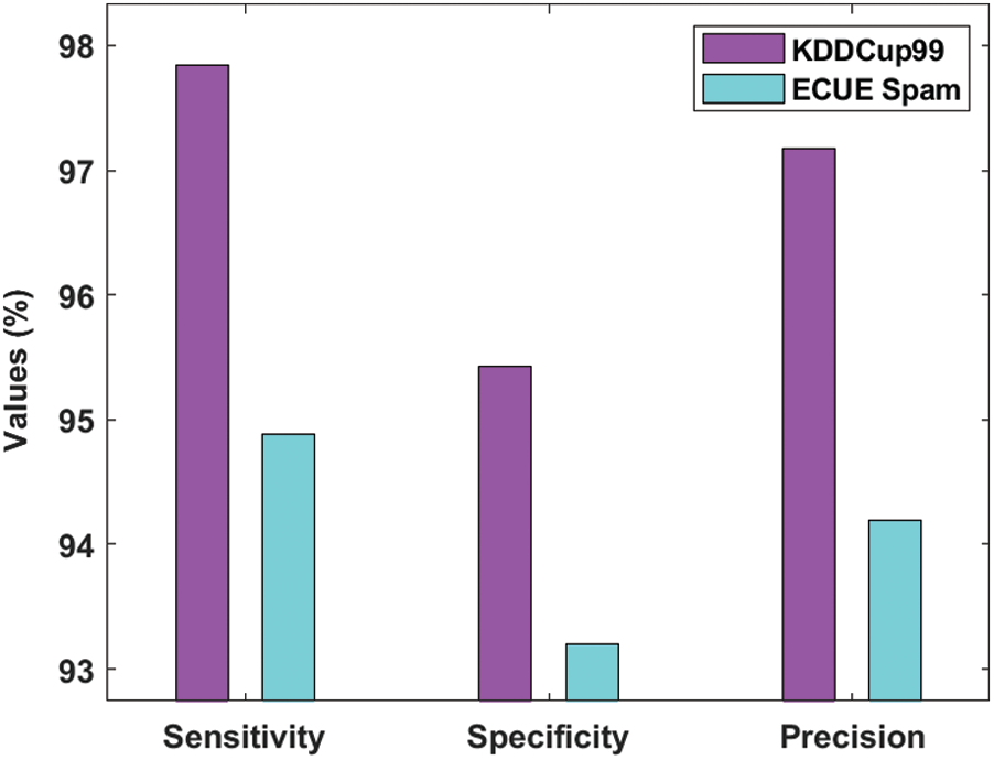
Figure 4: Result analysis of MOMBD-CDD model with different measures-I
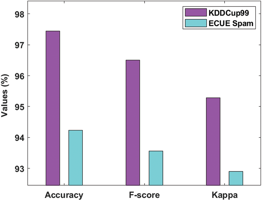
Figure 5: Result analysis of MOMBD-CDD model with different measures-II
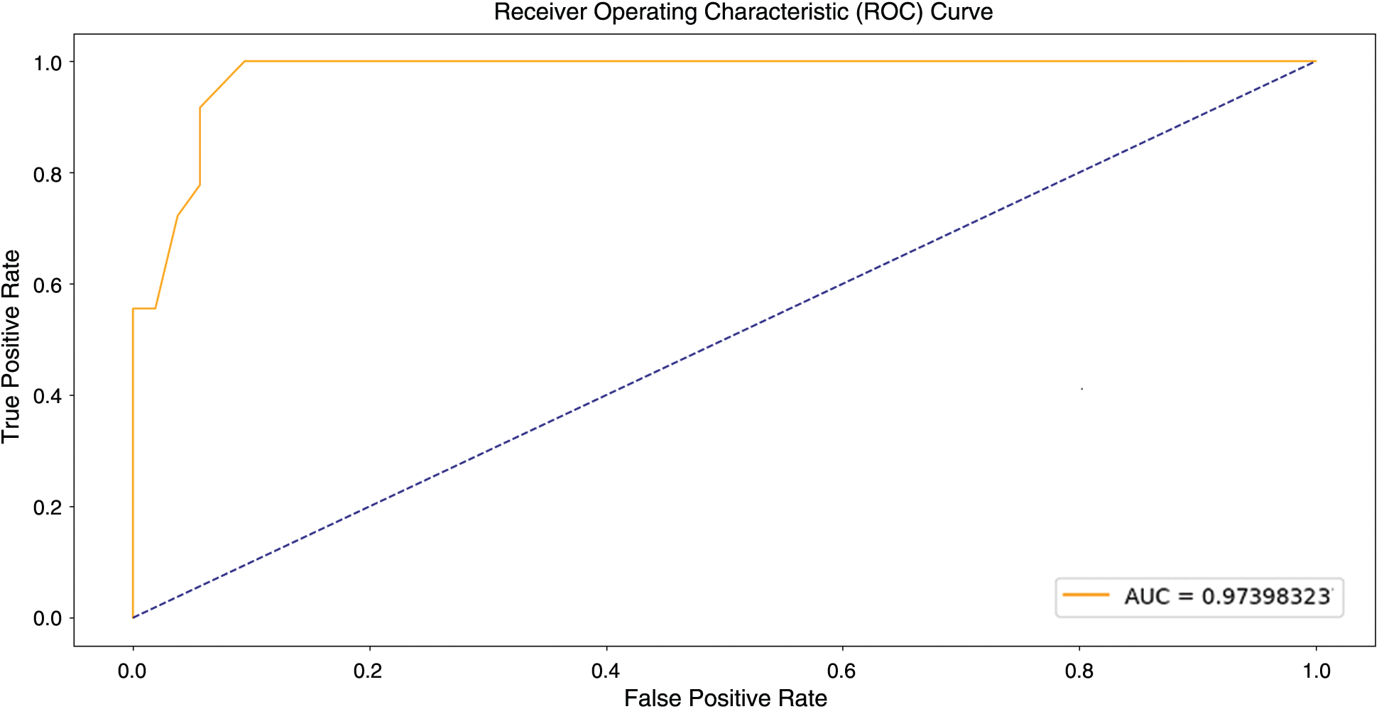
Figure 6: ROC analysis of KDDCup99 dataset on MOMBD-CDD
Fig. 6 illustrates the results of ROC analysis for MOMBD-CDD model on the applied test KDDCup99 dataset. From the figure, it is understood that the MOMBD-CDD model accomplished effective outcomes i.e., maximum AUC of 0.97398323.
Fig. 7 demonstrates the results of ROC analysis for MOMBD-CDD model upon the applied test ECUE Spam Dataset. From the figure, it is understood that the MOMBD-CDD model gained proficient performance as the model produced high AUC of 0.932389937.
Tab. 4 and Fig. 8 investigate the results of classification analysis of the MOMBD-CDD model upon applied KDDCup99 dataset [25]. The table values denote that the Gradient Boosting technique achieved only the least accuracy of 84.30%. Besides, Naïve Bayesian model accomplished a slightly-increased accuracy of 89.60%. At the same time, Random Forest model obtained a moderate accuracy of 90.24%. Likewise, the OC-SVM and Gaussian Process models too demonstrated closer accuracy values of 91.80% and 91.10% respectively. Simultaneously, the DNN-SVM model exhibited a competitive accuracy of 92%. Among these, the MOMBD-CDD model accomplished effective outcomes with high accuracy of 97.45%.
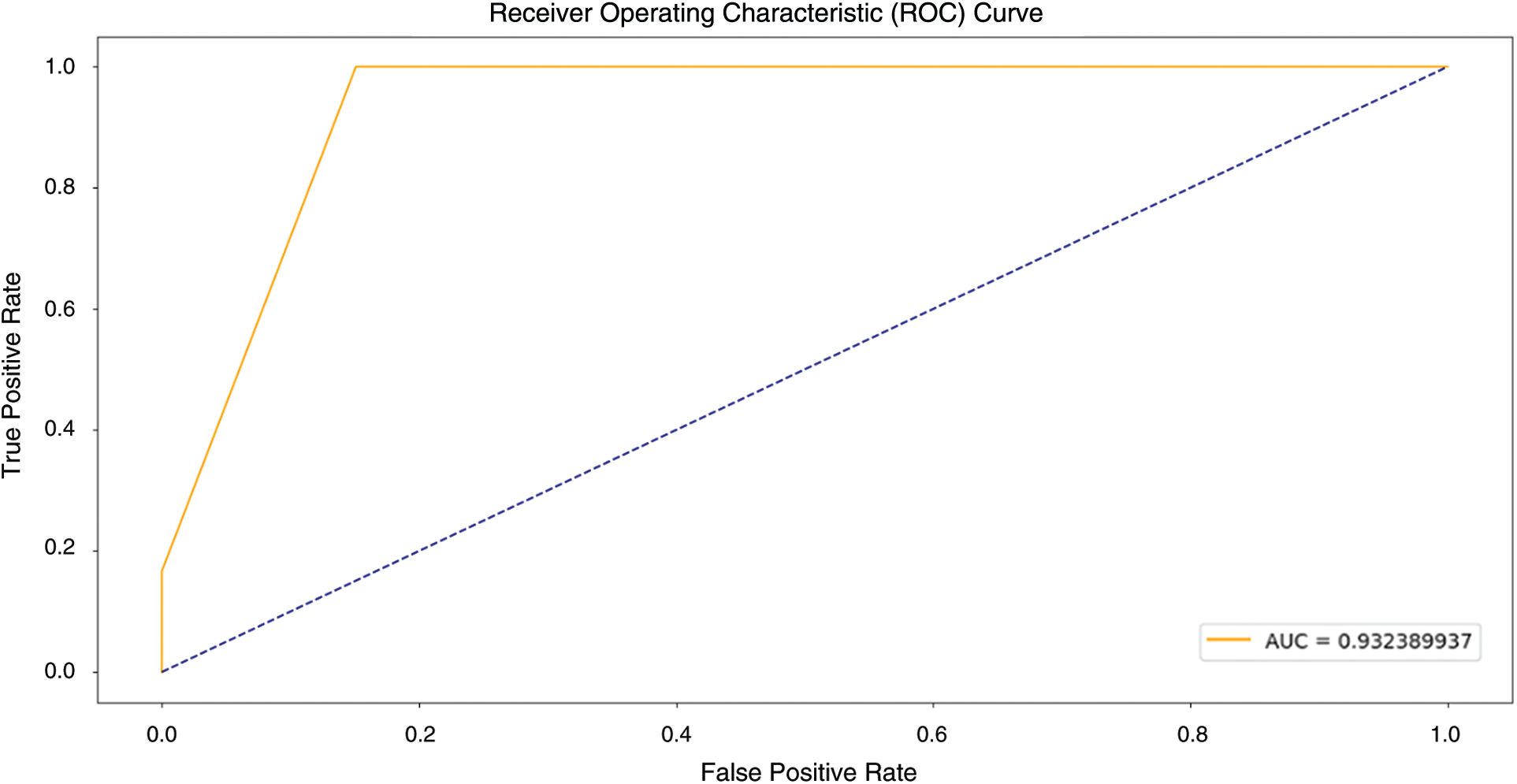
Figure 7: ROC analysis on ECUE spam dataset on MOMBD-CDD
Table 4: Performance comparison of the proposed method with recent methods on KDDCup99 dataset
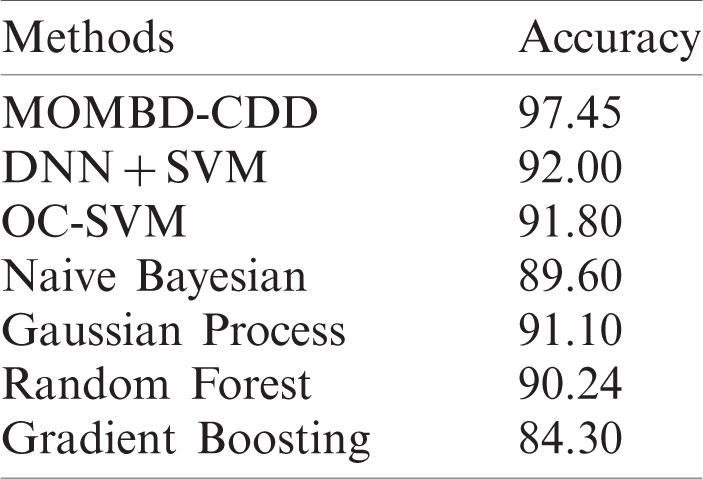
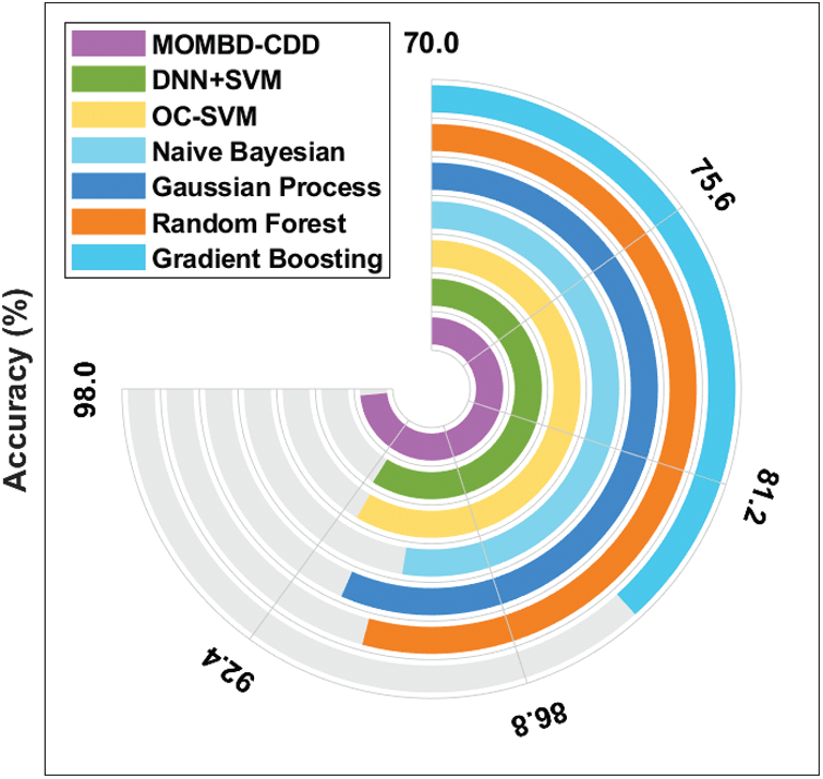
Figure 8: Accuracy analysis of MOMBD-CDD model on KDDCup99 dataset
Table 5: Performance evaluation of the proposed method with recent methods on ECUE spam dataset
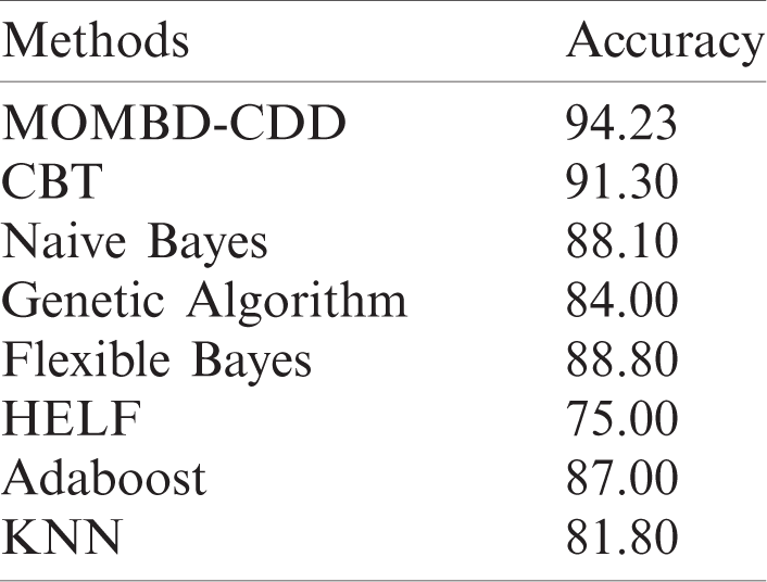
Tab. 5 and Fig. 9 examine the outcomes of classification analysis for MOMBD-CDD method upon the applied ECUE spam dataset [26–29]. The table values correspond that the HELF technique resulted in minimum accuracy of 75%. Besides, the KNN model resulted in somewhat higher accuracy of 81.80%. At the same time, the Genetic algorithm model attained a moderate accuracy of 84%. In line with this, the Adaboost model also showcased an even better result with an accuracy of 87%.
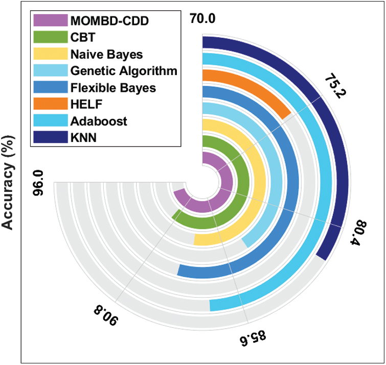
Figure 9: The accuracy analysis of MOMBD-CDD model on ECUE spam dataset
Likewise, Naive Bayes and Flexible Bayes models also accomplished close accuracy values of 88.10% and 88.80% respectively. Simultaneously, CBT model exhibited a competitive accuracy value of 91.30%. At last, the MOMBD-CDD model accomplished the best effective results with high accuracy of 94.23%. From the above discussed results, it is evident that the MOMBD-CDD model accomplished superior results over other methods.
This research work proposed a novel MOMBD-CDD model for High-Dimensional Big Streaming Data. The presented MOMBD-CDD model has different operational stages namely, pre-processing, CDD, and classification. At first, online streaming big data was preprocessed to transform the raw streaming data into a compatible format. Then, the preprocessed data underwent class imbalance handling process with the help of SMOTE-GSO algorithm. Followed by, the CDD process was incorporated with the help of STEPD technique. Finally, the classification task was performed by Bi-LSTM model and further tuned by GSO algorithm to determine the hyperparameters. The model was extensively validated through experiments which confirmed that the proposed model can produce effective outcome. The presented MOMBD-CDD model attained high accuracies of 97.45% and 94.23% on the applied datasets i.e., KDDCup99 Dataset and Spam dataset respectively. In future, the performance can be increased through clustering and feature selection techniques.
Funding Statement: The authors received no specific funding for this study.
Conflicts of Interest: The authors declare that they have no conflicts of interest to report regarding the present study.
1. I. Žliobaite, “Learning under concept drift: An overview,” Technical report, Faculty of Mathematics and Informatics, Vilnius University, Vilnius, Lithuania, 2009. [Google Scholar]
2. R. S. M. Barros, D. R. L. Cabral, P. M. Gonçalves Jr. and S. G. T. C. Santos, “RDDM: Reactive drift detection method,” Expert Systems with Applications, vol. 90, pp. 344–355, 2017. [Google Scholar]
3. P. Li, X. Wu, X. Hu and H. Wang, “Learning concept-drifting data streams with random ensemble decision trees,” Neurocomputing, vol. 166, no. 3, pp. 68–83, 2015. [Google Scholar]
4. J. Ross, N. M. Adams, D. K. Tasoulis and D. J. Hand, “Exponentially weighted moving average charts for detecting concept drift,” Pattern Recognition Letters, vol. 33, no. 2, pp. 191–198, 2012. [Google Scholar]
5. G. Widmer and M. Kubat, “Learning in the presence of concept drift and hidden contexts,” Machine Learning, vol. 23, no. 1, pp. 69–101, 1996. [Google Scholar]
6. S. Liu, L. Feng, J. Wu, G. Hou and G. Han, “Concept drift detection for data stream learning based on angle optimized global embedding and principal component analysis in sensor networks,” Computers & Electrical Engineering, vol. 58, no. 8, pp. 327–336, 2017. [Google Scholar]
7. A. Bifet and R. Gavaldà, “Learning from time-changing data with adaptive windowing,” in Society for Industrial and Applied Mathematics. Int. Conf. on Data Mining, Minnesota, USA, 2007. [Google Scholar]
8. S. Xu and J. Wang, “Dynamic extreme learning machine for data stream classification,” Neurocomputing, vol. 238, no. 99, pp. 433–449, 2017. [Google Scholar]
9. J. L. Lobo, I. Laña, J. D. Ser, M. N. Bilbao and N. Kasabov, “Evolving spiking neural networks for online learning over drifting data streams,” Neural Networks, vol. 108, no. 12, pp. 1–19, 2018. [Google Scholar]
10. Y. Zhang, G. Chu, P. Li, X. Hu and X. Wu, “Three-layer concept drifting detection in text data streams,” Neurocomputing, vol. 260, no. 3, pp. 393–403, 2017. [Google Scholar]
11. J. L. Lobo, J. D. Ser, M. N. Bilbao, C. Perfecto and S. S. Sanz, “DRED: An evolutionary diversity generation method for concept drift adaptation in online learning environments,” Applied Soft Computing, vol. 68, pp. 693–709, 2018. [Google Scholar]
12. B. Mirza, Z. Lin and N. Liu, “Ensemble of subset online sequential extreme learning machine for class imbalance and concept drift,” Neurocomputing, vol. 149, no. 9, pp. 316–329, 2015. [Google Scholar]
13. E. Arabmakki and M. Kantardzic, “SOM-based partial labeling of imbalanced data stream,” Neurocomputing, vol. 262, pp. 120–133, 2017. [Google Scholar]
14. J. L. Lobo, J. D. Ser, M. N. Bilbao, I. Laña and S. S. Sanz, “A probabilistic sample matchmaking strategy for imbalanced data streams with concept drift,” in Int. Symp. on Intelligent and Distributed Computing IDC 2016: Intelligent Distributed Computing X, Cham, Springer, vol. 678, pp. 237–246, 2016. [Google Scholar]
15. T. S. Sethi and M. Kantardzic, “On the reliable detection of concept drift from streaming unlabeled data,” Expert Systems with Applications, vol. 82, no. 12, pp. 77–99, 2017. [Google Scholar]
16. J. De Andrade Silva, E. R. Hruschka and J. Gama, “An evolutionary algorithm for clustering data streams with a variable number of clusters,” Expert Systems with Applications, vol. 67, no. 1, pp. 228–238, 2017. [Google Scholar]
17. I. Kim and C. H. Park, “Concept drift detection on streaming data under limited labeling,” in IEEE Int. Conf. on Computer and Information Technology, Nadi, Fiji, pp. 1–9, 2016. [Google Scholar]
18. V. Chawla, K. W. Bowyer, L. O. Hall and W. P. Kegelmeyer, “SMOTE: Synthetic minority over-sampling technique,” Journal of Artificial Intelligence Research, vol. 16, pp. 321–357, 2002. [Google Scholar]
19. J. Wang, B. Makond, K. H. Chen and K. M. Wang, “A hybrid classifier combining SMOTE with PSO to estimate 5-year survivability of breast cancer patients,” Applied Soft Computing, vol. 20, pp. 15–24, 2014. [Google Scholar]
20. N. Krishnan and D. Ghose, “Glowworm swarm optimization for searching higher dimensional spaces,” in Innovations in Swarm Intelligence, vol. 248. Berlin, Heidelberg: Springer, pp. 61–75, 2009. [Google Scholar]
21. D. R. De Lima Cabral and R. S. M. De Barros, “Concept drift detection based on fisher’s exact test,” Information Sciences, vol. 442–443, pp. 220–234, 2018. [Google Scholar]
22. N. Yulita, M. I. Fanany and A. M. Arymuthy, “Bi-directional long short-term memory using quantized data of deep belief networks for sleep stage classification,” Procedia Computer Science, vol. 116, pp. 530–538, 2017. [Google Scholar]
23. KDD Cup 1999 Data, The Third International Knowledge Discovery and Data Mining Tools Competition. [Online]. Available: http://kdd.ics.uci.edu/databases/kddcup99/kddcup99.html (Accessed June 14, 2020). [Google Scholar]
24. ECUE Spam dataset, [Online]. Available: http://www.comp.dit.ie/sjdelany/dataset.htm (Accessed June 14, 2020). [Google Scholar]
25. H. Hindy, R. Atkinson, C. Tachtatzis, J. N. Colin and E. Bayne, “Utilising deep learning techniques for effective zero-day attack detection,” Electronics, vol. 9, no. 10, pp. 1–16, 2020. [Google Scholar]
26. J. Delany, P. Cunningham, A. Tsymbal and L. Coyle, “A case-based technique for tracking concept drift in spam filtering,” Knowledge-Based Systems, vol. 18, no. 4–5, pp. 187–195, 2005. [Google Scholar]
27. N. Pérez-Díaz, D. Ruano-Ordás, F. Fdez-Riverola and J. R. Méndez, “Boosting accuracy of classical machine learning antispam classifiers in real scenarios by applying rough set theory,” Scientific Programming, vol. 2016, pp. 1–10, 2016. [Google Scholar]
28. C. Zhao, Y. Xin, X. Li, Y. Yang and Y. Chen, “A heterogeneous ensemble learning framework for spam detection in social networks with imbalanced data,” Applied Sciences, vol. 10, no. 3, pp. 1–18, 2020. [Google Scholar]
29. N. Saidani, K. Adi and M. S. Allili, “A semantic-based classification approach for an enhanced spam detection,” Computers & Security, vol. 94, no. 1, pp. 101716, 2020. [Google Scholar]
 | This work is licensed under a Creative Commons Attribution 4.0 International License, which permits unrestricted use, distribution, and reproduction in any medium, provided the original work is properly cited. |