Computers, Materials & Continua DOI:10.32604/cmc.2021.016539
Article

Unsupervised Domain Adaptation Based on Discriminative Subspace Learning for Cross-Project Defect Prediction

Ying Sun1, Yanfei Sun*,1,2, Jin Qi1, Fei Wu1, Xiao-Yuan Jing1,3, Yu Xue4 and Zixin Shen5

1Nanjing University of Posts and Telecommunications, Nanjing, 210003, China
2Jiangsu Engineering Research Center of HPC and Intelligent Processing, Nanjing, 210003, China
3Wuhan University, Wuhan, 430072, China
4Nanjing University of Information Science and Technology, Nanjing, 210044, China
5Carnegie Mellon University, Pittsburgh, 15213, USA
*Corresponding Author: Yanfei Sun. Email: sunyanfei@njupt.edu.cn
Received: 04 January 2021; Accepted: 26 February 2021

Abstract: Cross-project defect prediction (CPDP) aims to predict the defects on target project by using a prediction model built on source projects. The main problem in CPDP is the huge distribution gap between the source project and the target project, which prevents the prediction model from performing well. Most existing methods overlook the class discrimination of the learned features. Seeking an effective transferable model from the source project to the target project for CPDP is challenging. In this paper, we propose an unsupervised domain adaptation based on the discriminative subspace learning (DSL) approach for CPDP. DSL treats the data from two projects as being from two domains and maps the data into a common feature space. It employs cross-domain alignment with discriminative information from different projects to reduce the distribution difference of the data between different projects and incorporates the class discriminative information. Specifically, DSL first utilizes subspace learning based domain adaptation to reduce the distribution gap of data between different projects. Then, it makes full use of the class label information of the source project and transfers the discrimination ability of the source project to the target project in the common space. Comprehensive experiments on five projects verify that DSL can build an effective prediction model and improve the performance over the related competing methods by at least 7.10% and 11.08% in terms of G-measure and AUC.

Keywords: Cross-project defect prediction; discriminative subspace learning; unsupervised domain adaptation

1  Introduction

Software security is important in the software product development process. Defects are inevitable and damage the high quality of the software. Software defect prediction (SDP) [1–3] is one of the most important steps in software development and can detect potentially defective instances before the release of software. Recently, SDP has received much research attention.

Most SDP methods construct a prediction model based on historical defect data and then apply it to predict the defects of new instances within the same project, which is called within-project defect prediction (WPDP) [4–6]. The labeled historical data, however, usually are limited. New projects have few historical data, and the collection of labels is time-consuming. However, plenty of data are available from other projects, and cross-project defect prediction (CPDP) [7,8] has emerged as an alternative solution.

CPDP uses training data from external projects (i.e., source projects) to train the prediction model, and then predicts defects in the target project [9]. CPDP is challenging because a prediction model that is trained on one project might not work well on other projects. Huge gaps exist between different projects because of differences in the programming language used, developer experience levels, and code standards. Zimmermann et al. [7] performed CPDP on 622 pairs of projects, and only 21 pairs performed well. In the machine learning literature [10], such works always require different projects to have similar distribution. In WPDP, this assumption is easy, but it cannot hold for CPDP. Therefore, the ability to reduce the distribution differences between different projects is key to increasing the effectiveness of CPDP.

To overcome this distribution difference problem, many methods have been proposed. Some researchers have used data filtering techniques. For example, Turhan et al. [11] used the nearest neighbor technique to choose instances from the source project that were similar to instances from the target project. Some researchers have introduced transfer learning methods into CPDP. For example, Nam et al. [12] used transfer component analysis to reduce the distribution gaps between different projects. These works usually have ignored the consideration of conditional distributions of different projects.

Unsupervised domain adaptation (UDA) [13,14] focuses on knowledge transfer from the source domain to the target domain, with the aim of decreasing the discrepancy of data distribution between two domains, which is widely used in various fields, such as computer vision [15], and natural language processing [14]. The key to UDA is to reduce the domain distribution difference. Subspace learning is the main category of UDA, which can conduct subspace transformation to obtain better feature representation. In addition, most existing CPDP methods ignore the effective exploration of class label information from the source data [11].

In this paper, to reduce the distribution gap across projects and make full use of the class label information of source project, we propose a discriminative subspace learning (DSL) approach based on UDA for CPDP. DSL aims to align the source and target projects into a common space by feature mapping. In addition, DSL incorporates class-discriminative information into the learning process. We conduct comprehensive experiments on five projects to verify that DSL can build an effective prediction model and improve the performance over the related competing methods by at least 7.10% and 11.08% in terms of G-measure and AUC, respectively. Our contributions are as follows:

1.    We propose a discriminative subspace learning approach for CPDP. To reduce the distribution gap of the data between source and target projects, DSL uses subspace learning based on UDA to learn a projection that can map the data from different projects into the common space.

2.    To fully use the label information and ensure that the model has better discriminative representation ability, DSL incorporates discriminative feature learning and accurate label prediction into subspace learning procedure for CPDP.

3.    We conduct extensive experiments on 20 cross-project pairs. The results indicate the effectiveness and the superiority of DSL compared with related baselines.

The remainder of this paper is organized as follows. The related works are discussed in Section 2. The details of DSL are introduced in Section 3. The experiment settings are provided in Section 4. Section 5 gives the experimental results and analysis. Section 6 analyzes the threats to the validity of our study. The study is concluded in Section 7.

2  Related Work

In this section, we review the related CPDP methods and subspace learning based unsupervised domain adaptation methods.

2.1 Cross-Project Defect Prediction

Over the past several years, CPDP has attached many studies and many new methods have been proposed. Briand et al. [16] first proposed whether the cross system prediction model can be investigated. They developed a prediction model on one project and then used it for other projects. The poor experimental results showed that applying models across projects is not easy.

Some methods focus on designing an effective machine learning model with an improved learning ability or generalization ability. Xia et al. [8] proposed a hybrid model (HYDRA) including genetic algorithm and ensemble learning. In the genetic algorithm stage, HYDRA builds multiple classifiers and assigns weights to different classifiers to output an optimal composite model. In ensemble learning phase, the weights of instances can be updated by iteration to learn a composition of the previous classifiers. Wu et al. [17] employed dictionary learning in CPDP and proposed an improved dictionary learning method CKSDL for addressing class imbalanced problem and semi-supervised problem. The authors utilize semi-supervised dictionary learning to improve the feature learning ability of the prediction model. CKSDL combines cost-sensitive technique and kernel technique to further improve the prediction model. Then, Sun et al. [18] introduced adversarial learning into CPDP and embedded a triplet sampling strategy into an adversarial learning framework.

In addition, some methods focus on introducing transfer learning into CPDP. Ma et al. [19] proposed transfer naive bayes for CPDP. They exploited the transfer information from different projects to construct weighted training instances, and then built a prediction model on these instances. The experiment indicated that useful transfer knowledge would be helpful. Nam et al. [12] employed transfer component analysis for CPDP, which learns transfer components in a kernel space to make the data distribution from different projects similar, and an experiment on two datasets indicated that TCA+ achieves good performance. Li et al. [20] proposed cost-sensitive transfer kernel canonical correlation analysis (CTKCCA) to mitigate the linear inseparability problem and class imbalance problem in heterogeneous CPDP. They introduced CCA into heterogeneous CPDP and improved the CCA to obtain better performance. Liu et al. [21] proposed a two-phase method called TPTL based on transfer learning, which can address the instability issue of traditional transfer learning. TPTL first selects source projects that have high similarity with target project. Then, TPTL uses TCA+ in the prediction model on the selected source projects.

Hosseini et al. [22] evaluated 30 previous studies, including their data metrics, models, classifiers and corresponding performance. The authors counted the common settings and concluded that CPDP is still a challenge and has room for improvement. Zhou et al. [23] compared the performance of existing CPDP methods. In addition, they built two unsupervised models—ManualUp and ManualDown, which only use the size of a module to predict its defect proneness. They concluded that the module size based models achieve good performance for CPDP.

Existing CPDP methods cannot consider the conditional distribution differences between different projects and ignore the discriminative information from both source project and target project. From the above consideration, we propose DSL to improve the performance of CPDP.

2.2 Unsupervised Domain Adaptation

Unsupervised domain adaptation has attracted much attention, and it aims to transfer useful information from the source to the target domain effectively in unsupervised scenario. Domain adaptation methods have been applied to various applications, such as computer vision [15] and natural language processing [14]. Subspace learning based unsupervised domain adaptation aims to learn a mapping for aligning the subspaces between two projects. Sun et al. [13] proposed subspaces distribution alignment method for performing subspace alignment to reduce distribution gaps. Long et al. [24] adapted both marginal distribution and conditional distribution between the source and target domains to reduce the different distributions simultaneously. Zhang et al. [25] proposed guided subspace learning to reduce the discrepancy between different domains.

In this paper, we introduce subspace learning based unsupervised domain adaptation into CPDP, which can effectively reduce the distribution gap between different projects. We also make full use of the class information from source project and propose a discriminative subspace learning approach for CPDP.

3  Methodology

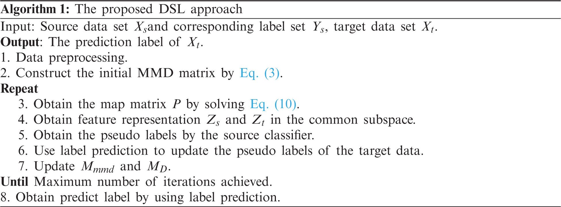
In this section, we present the details of DSL. Fig. 1 illustrates the overall framework of the proposed DSL approach for CPDP.

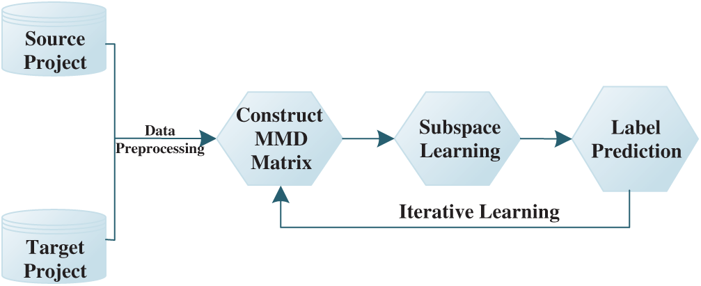
Figure 1: Framework of our proposed DSL approach for CPDP

3.1 Data Preprocessing

To alleviate the class imbalance problem, we perform SMOTE [26] technique on the source project, as is one of the most widely used data preprocessing methods in CPDP. Previous works [27,28] have demonstrated that dealing with the class imbalance problem is helpful for SDP.

3.2 Notation

Given the labeled source project S={Xs,Ys}={xsi,ysi}i=1ns and the unlabeled target project T={Xt}={xti}i=1nt, where Xs and Xt are the data sets and Ys is the label set. ns and nt are the numbers of instances from source and target projects, respectively. Here, xsi={asi1;asi2;…;asid} denotes the ith instance in the source project, and xti={ati1;ati2;…;atid} denotes the ith instance in target project. ysi is the corresponding label of xsi. asij denotes the value of the jth metric in the ith instance xsi in source project. atij denotes the value of the jth metric in the ith instance xti in the T source project; and d is the metric dimension of the source or target project. In CPDP, the labels of the target project Yt={yt1,yt2,…,ytnt} are unknown.

3.3 Subspace Learning

To minimize the distribution discrepancy between the projects, we seek an effective transformation P . We construct a common subspace with the projection P . The mapped representations with the projection matrix from the source and target projects are represented as zs = PTxs, and zt = PTxt, respectively.

To effectively reduce the distribution discrepancy between the different projects, we consider the distances of conditional distributions across the projects. The maximum mean discrepancy (MMD) criterion [29] has been used widely to measure the difference between two distributions. We minimize the distance Fmmd(S,T) between the source and target projects as follows:

Fmmd(S,T)=Fmmd(p(ys∣xs),p(y˜t∣xt))=∑c=1C‖ 1nsc∑i=1nsczsic−1ntc∑j=1ntcztjc ‖2(1)

where p(ys∣xs) and p(yt∣xt) denote the conditional distributions from the source and target projects. C denotes the number of label classes in CPDP. In this paper, the label of an instance is defective or non-defective, and C = 2 . nsc and ntc are the numbers of the instances from source and target projects in class c . Specifically, the label of the target instance is unknown in CPDP. A feasible method is to use the target pseudo label ỹt, which can be predicted by the source classifier. We can make full use of the intrinsic discriminative information of the target project during the training process. In addition, we employ multiple iterations to improve the accuracy of the predicted labels.

Using matrix tricks, we rewrite Eq. (1) as follows:

Fmmd(S,T)=∑c=1CTr(PTXMcXTP)=Tr(PTXMmmdXTP)(2)

where X={Xs,Xt} combines the source project and target project data, and Mmmd=∑c=1CMc. Mc denotes the conditional MMD matrix with class c , which is computed as

Mcij={1nscnsc,if xi,xj∈S1ntcntc,if xi,xj∈T-1nscntc,if {xi∈S,xj∈Txi∈T,xj∈S0,otherwise(3)

3.4 Discriminative Feature Learning

Minimizing Eq. (1) can align the source data and target data, but it cannot guarantee that the learned feature representations are sufficiently discriminative. To ensure that the feature representations from the same class are closer than those from different classes in the common space, we design a triplet constraint that minimizes the distance between the intra-class instances and maximizes the distances between the inter-class instances. This constraint is based on the prior assumption of consistency. This means that nearby instances are likely to have the same label.

Specifically, we focus on the hardest cases, which are the most dissimilar instances within the same class and the most similar instances in the different classes. For each instance zsi in the source project, we choose the farthest instance zsj with the same class as a positive matching, and the nearest instance zsk with a different class as a negative matching. Finally, we construct the triplet (zsi,zsj+,zsk-) for each instance in the source project. Then, we design the following formulation:

Fs=∑c=1C∑i=1nsc(minzjs‖ zsi−zsj ‖2−minzsk‖ zsi−zsk ‖2)=Tr(PTXs(Msintra−Msinter)XsTP)(4)

where Msintra and Msinter denote the distance between the instance pairs. Similarly, we define the triplet for the target instances in the same way and the formulation can be represented as

Ft=∑c=1C∑i=1ntc(minzjt‖ zti−ztj ‖2−minztk‖ zti−ztk ‖2)=Tr(PTXt(Mtintra−Mtinter)XtTP)(5)

We obtain the whole formula for the source and target projects as

FD=Fs+Ft=Tr(PTX(Mintra-Minter)XTP)=Tr(PTXMDXTP)(6)

We formulate the overall equation of the DSL by incorporating Eqs. (2) and (6) as follows:

F=Fmmd+αFD+β∥P∥F2(7)

where α is a balance factor and β is a regularization term.

The optimization of DSL is represented as follows:

minPTr(PTX(Mmmd+αMD)XTP)+β∥P∥F2s.t.PTXHXTP=I(8)

where I is an identity matrix and H=I-(1/n)1 denotes a centering matrix similar to that in [24]. The constraint condition ensures that PTX can preserve the inner attributes of the original data. The optimization problem of Eq. (8) can be solved as a generalized eigendecomposition problem. To solve Eq. (8), we denote Lagrange multipliers as Φ=(Φ1,Φ2,…,Φdl), and then we rewrite Eq. (8) as

LP=PTX(Mmmd+αMD)XTP+β∥P∥F2+(I-PTXHXTP)Φ(9)

We set the derivative of P to 0, and then we compute the eigenvectors for the generalized eigenvector problem:

(X(Mmmd+αMD)XT+βI)P=XHXTPΦ(10)

By solving Eq. (10), we can obtain the optimal transformation matrix P . We iteratively update P and M to benefit the next iteration process in a positive feedback way.

3.5 Label Prediction

To further improve the prediction accuracy of the target data, we design a label prediction mechanism. Considering that predicting target labels by using a source classifier directly may lead to overfitting, we utilize the label consistency between different projects and within the same project to obtain more accurate label prediction results.

In the common subspace, we believe that the classifier will be more accurate when the target instances are close to the source instances. Moreover, similar instances should have consistent labels. We assign larger weights to similar target instances that are close to the source instances, and assign smaller weights to dissimilar target instances that are far from the source instances.

The formula for label prediction can be defined as

minft∑i=1ntλi(fs(zti)-ft(zti))2+∑i,j=1ntwij(ft(zti)-ft(ztj))2(11)

where fs(zti) is the prediction label for zti from the source classifier. ft(zti) is the expected label for zti. λi is a weight factor for ztic⋅wij is a binary matrix that is used to measure the similarity between different instances from the target project. If the ith instance and jth instance are nearest neighbor, the value of wij is 1, otherwise the value of wij is 0. λi can be calculated by the following formula:

λi=ntntc⋅11+ exp(lic)(12)

where nt/ntc is used to balance the effects of different classes. lic denotes the distance between the target instance with pseudo label c predicted by the source classifier and the instance with an expect label c .

For simplicity, we define fs={fs(zt1),…,fs(ztnt)}, ft={ft(zt1),…,ft(ztnt)} and Λ=diag(λ1,…,λnt). We introduce the Laplacian matrix L = D − W , where W=∑i,j=1ntwij and Dii=∑j=1ntwij. Then, we rewrite Eq. (11) as

minft(ft-fs)TΛ(ft-fs)+ftTLft(13)

Then, we obtain the solution of (13) as ŷ=(Zt(Λ+L)ZtT)-1ZtΛfs. The label of zti is ft(zti)=(ŷ)Tzti. We summarize the DSL approach in Algorithm 1.

4  Experiment

4.1 Dataset

We adopt five widely used projects from the AEEEM dataset [30] for CPDP. The AEEEM dataset is collected by D’Ambros et al. [30] and contains the data about Java projects. The projects of AEEEM are Equinox (EQ), Eclipse JDT Core (JDT), Apache Lucene (LC), Mylyn (ML) and Eclipse PDE UI (PDE). Each project consists of 61 metrics including entropy code metrics, source code metrics, etc. The data is publicly available online: http://bug.inf.usi.ch/. Tab. 1 shows the detailed information for each project.

4.2 Evaluation Measures

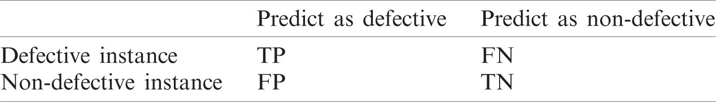
In the experiment, we employ two well-known measures, the G-measure and AUC, to evaluate the performance of the CPDP model; these have been widely used in previous SDP works [20,31]. The G-measure is a harmonic mean of recall (aka. pd) and specificity, and it is defined in Eq. (14). Recall is a measure defined as TP/(TP+FN). Specificity is a statistical measure that is defined as TN/(TN+FP). TP, FN, TN, and FP mean True Positive, False Negative, True Negative and False Positive, respectively, and they are defined in Tab. 2.

G-measure=2×recall×specificity(recall+specificity)(14)

The AUC is used to evaluate the performance of the classification model. The ROC curve is a two-dimensional plane with recall and pf. Pf, i.e., the possibility of false alarm, which is defined as FP/(TN+FP). The AUC calculates the area under ROC curve.

The values of the G-measure and AUC range from 0 to 1. A higher value means better prediction performance. AUC=0.5 signifies a model that is randomly guessing.

Table 1: Experimental data description

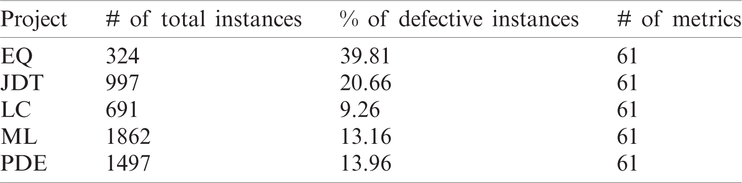
Table 2: Four kinds of defect prediction results

4.3 Research Question

In this paper, we answer the following research question:

RQ: Does DSL outperform previous related works?

We compare DSL with defect prediction models including TCA+ [12], CKSDL [17], CTKCCA [20] and ManualDown [23]. TCA+, CKSDL and CTKCCA are successful CPDP methods. ManualDown is an unsupervised method that was suggested as the baseline for comparison in [23] when developing a new CPDP method.

4.4 Experimental Setup

Similar to prior CPDP methods [17,20], we count cross-project pairs to perform CPDP. For each target project, there are four prediction combinations. For example, when EQ is selected as the target project, JDT, LC, ML and PDE are separately selected as source project for training. The prediction combinations are JDT→EQ, LC→EQ, ML→EQ, and PDE→EQ. We can obtain 20 cross-project pairs for the five projects. In DSL, we set α=1 and β=0.1 in Eq. (10) empirically. We fix the maximum number of iterations to 10 in experiment.

5  Experimental Results and Analysis

5.1 RQ: Does DSL Outperform Previous Related Works?

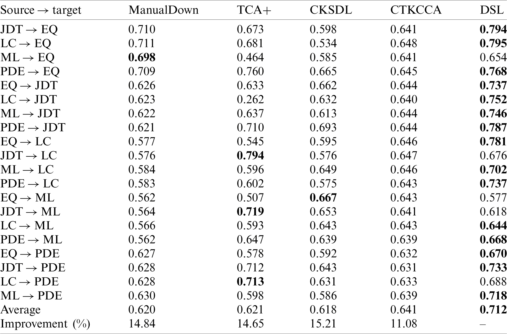
Tabs. 3 and 4 show the G-measure and AUC results of DSL and the baselines for each cross-project pair. The best result of each combination is in boldface. Fig. 2 shows the boxplots of G-measure and AUC for DSL and the baselines. From Tabs. 3 and 4 and Fig. 2, it is evident that DSL performs best in most cases compared with the baselines and obtains the best average result in terms of G-measure and AUC. In terms of the overall performance, DSL improves the average G-measure values by 7.10%–19.96% and average AUC values by 11.08%–15.21%.

Table 3: Comparison results in terms of G-measure for DSL and baselines. The best values are in boldface

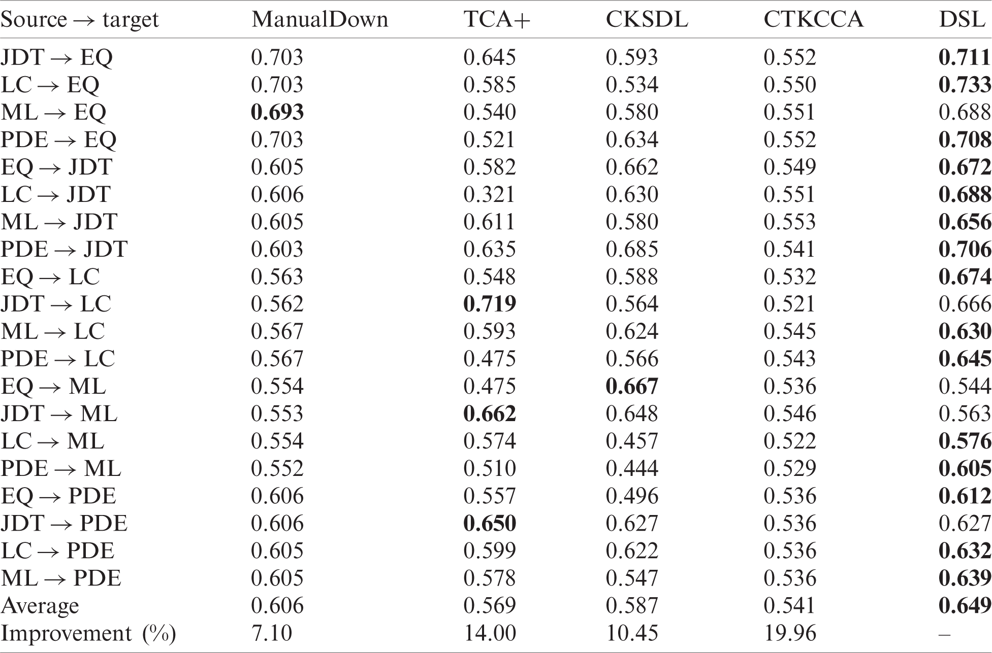
DSL obtains good performance may for the following reasons: Compared with TCA+ and CTKCCA, which reduce the distribution gap based on transfer learning, DSL embeds the discrimination representation into the feature learning process, and obtains discriminative common feature space that can reduce the distribution gap of data from different projects. Compared with ManualDown, DSL can utilize the class label information from the source project and discriminant information from the target project, which then obtain more useful information for the model training process. Compared with CKSDL, DSL can align the data distributions between different projects and has strong discriminative ability that can transfer it from the source project to the target project. Thus, in most cases, DSL outperforms the baselines.

Table 4: Comparison results in terms of AUC for DSL and baselines. The best values are in boldface

5.2 Statistical Test

We perform the Friedman test [32] with the Nemenyi test on the two measure results to analyze the statistical difference between DSL and baselines, which has been widely used in SDP [33,34]. For each evaluation measure, we compute the ranking of comparison methods on each cross-project pair. We apply Friedman test to determine whether the methods are significantly different. Then we apply Nemenyi test to compare the difference among each pair of methods. For a method pair, we compute their difference in rank by using critical difference (CD) value. If the difference in rank exceeds CD, we consider that the methods have significant difference. CD is defined as

CD=qαL(L+1)6N(15)

where qα denotes the critical value at significance level α, N is the number of cross-project pairs, and L denotes the number of methods.

The Friedman test results on the G-measure and AUC are visualized in Figs. 3 and 4 respectively. A lower rank means better performance. The methods that have significant differences are divided into different groups. As shown in Figs. 3 and 4, DSL performs better than the baselines with lower ranks. For the G-measure and AUC, DSL belongs to the top-ranked group without other methods, which means that it achieves the best performance, and that DSL has significant differences when compared with the baselines.

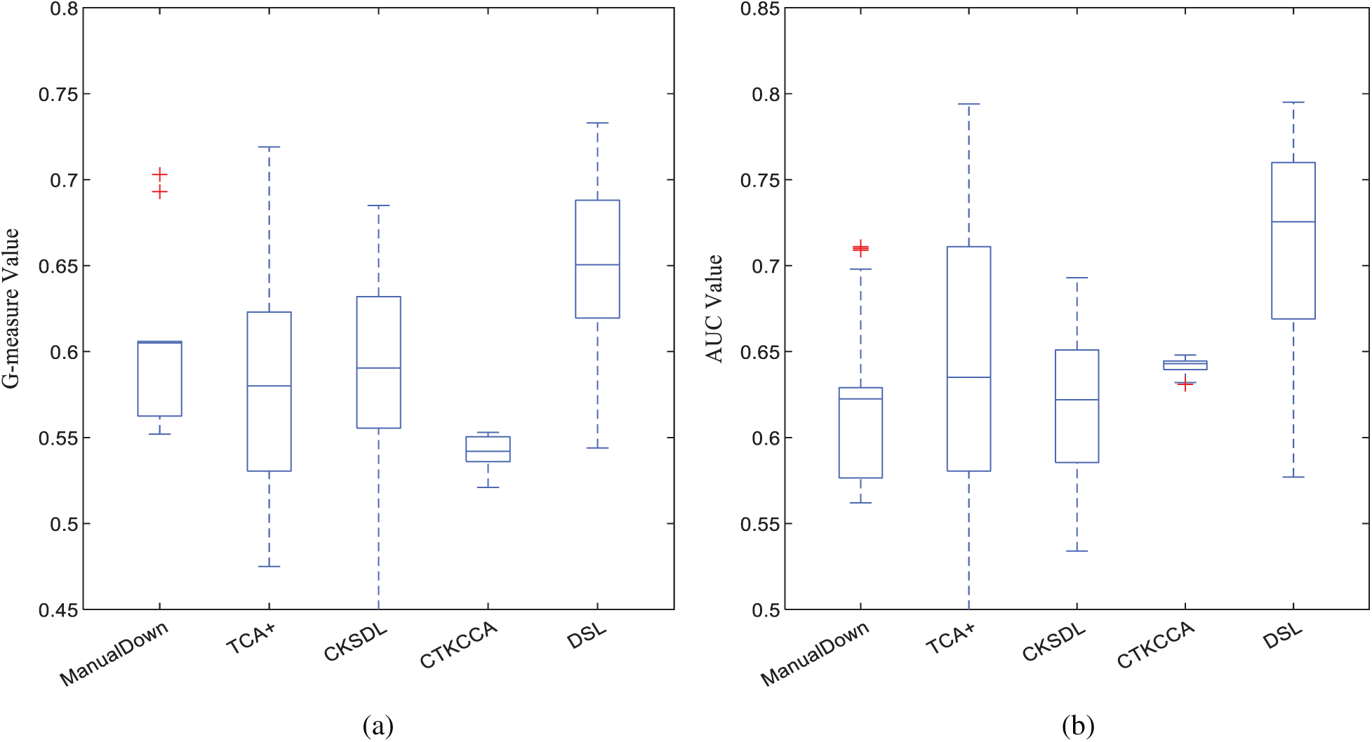
Figure 2: Boxplots of G-measure and AUC values across all projects for the baselines. (a) Boxplots of G-measure values. (b) Boxplots of AUC values

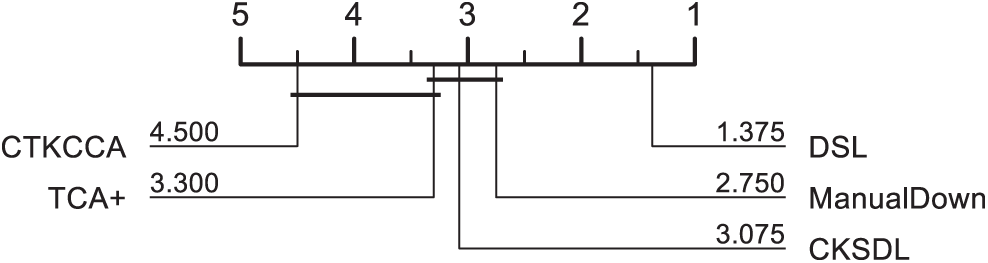
Figure 3: The results of statistical test in terms of G-measure for DSL and the other methods

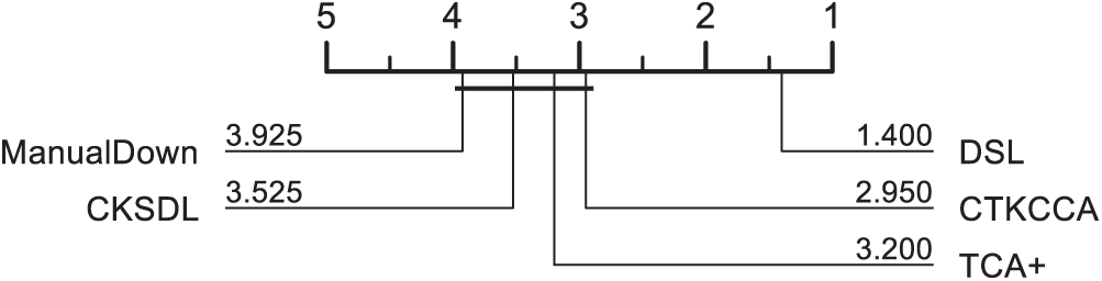
Figure 4: The results of statistical test in terms of AUC for DSL and the other methods

5.3 Ablation Study

To deeply investigate the impact of different parts of DSL, we conduct an ablation study. We evaluate DSL and two variants of DSL:

Subspace learning (DSL1): Using subspace learning based on conditional distribution for CPDP.

Subspace learning and discriminative feature learning (DSL2): Using subspace learning and discriminative feature learning for CPDP.

The experimental settings are the same as those in Section 4.4 on 20 cross-project combinations. The results are reported in Figs. 5 and 6. From the figures, the results of DSL are improved on different projects. Clearly, in the mapped feature space, the distribution difference is reduced. Discriminative learning can help us explore the discrimination between different classes. The pseudo labels provided by label prediction can facilitates subspace learning and discriminative feature learning. Thus, discriminative feature learning and label prediction boost each other during the iteration process. Discriminative feature learning and label prediction play important roles in exploring discriminative information for CPDP.

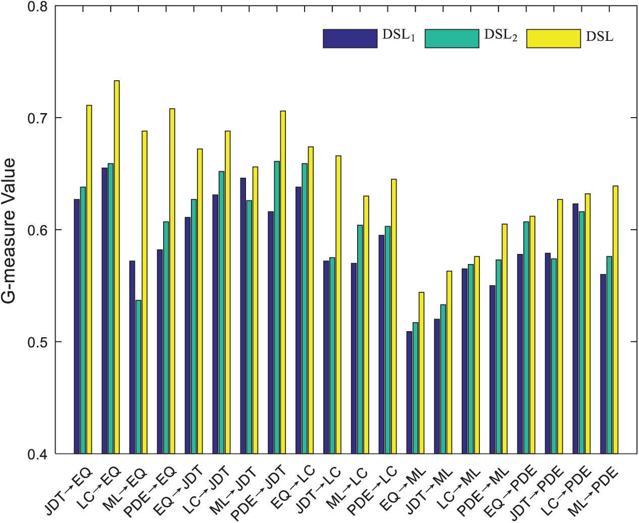
Figure 5: G-measure values of DSL and its variants on each project pair

5.4 Effects of Different Parameter Values

We conduct parameter sensitivity studies to verify the impact of parameters α and β on DSL. The value ranges of α and β are from 0.001 to 10. We report the experimental results in terms of the G-measure and AUC in Fig. 7.

From Fig. 7, we can observe that DSL achieves good performance under a wide range of values. When α∈[0.5,5] and β∈[0.05,0.5], DSL performs stably and outperforms the other cases. The results are not very sensitive to the parameters, which demonstrates the robustness of DSL. In the experiments, we set α=1 and β=0.1.

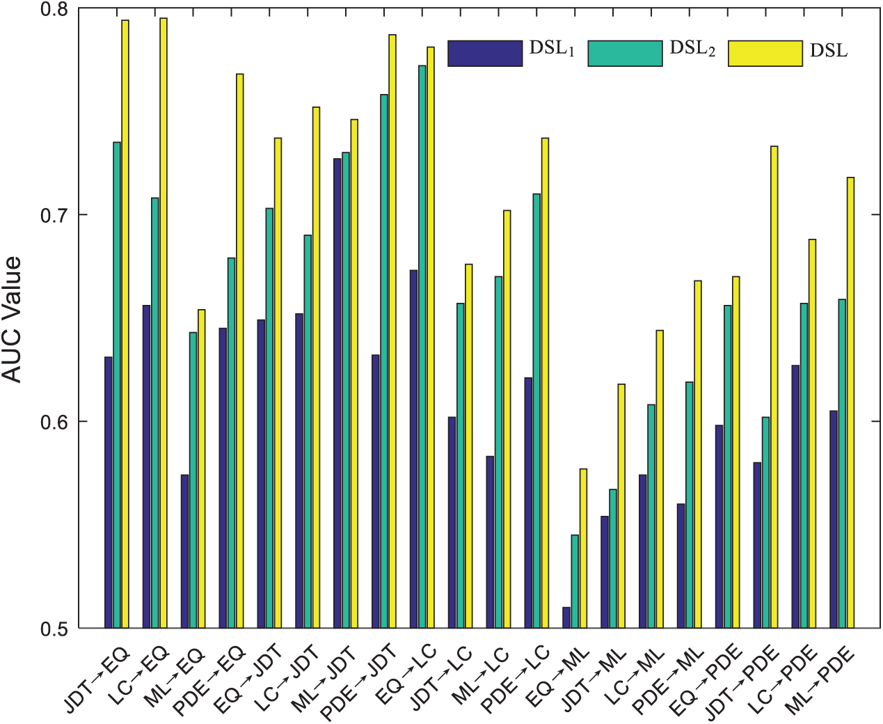
Figure 6: AUC values of DSL and its variants on each project pair

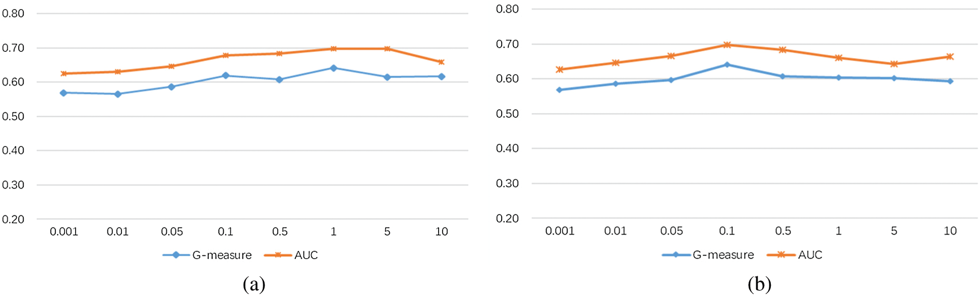
Figure 7: The mean G-measure and AUC values with various values of α and β. (a) Parameter α. (b) Parameter β

6  Threats to Validity

Internal validity mainly relates to the implementation of comparative baselines. For the baselines whose source codes can be provided by the original authors, we use the original implementation code to avoid the inconsistency of re-implementation. For the baselines do not public codes, we follow their papers and implement the methods carefully.

Construct validity in this work refers to the suitability of the evaluation measures. We employ two widely used measures and the selected measures are comprehensive indicators for CPDP.

External validity refers to the degree to which the results in this paper can be generalized to other tasks. We perform a comprehensive experiment on 5 projects in this paper. However, we still cannot claim that our approach would be suitable for other software projects.

7  Conclusion

In this paper, we propose a new model for CPDP based on unsupervised domain adaptation called discriminative subspace learning (DSL). DSL first handles the problem of large distribution gap in the feature mapping process. Furthermore, the discriminative feature learning is embedded in the feature mapping to make good use of the discriminative information from source project and target project. Extensive experiments on 5 projects are conducted. The performance of DSL is evaluated by using two widely used indicators including G-measure and AUC. The comprehensive experimental results show that DSL has superiority in CPDP. In our future work, we will focus on collecting more projects to evaluate DSL and predicting the number of defects in each instance by utilizing the defect count information.

Funding Statement: This paper was supported by the National Natural Science Foundation of China (61772286, 61802208, and 61876089), China Postdoctoral Science Foundation Grant 2019M651923, and Natural Science Foundation of Jiangsu Province of China (BK0191381).

Conflicts of Interest: No conflicts of interest exit in the submission of this manuscript, and manuscript is approved by all authors for publication.

References

 1.  Ö.F. Arar and K. Ayan, “Software defect prediction using cost-sensitive neural network,” Applied Soft Computing, vol. 33, no. 1, pp. 263–277, 2015. [Google Scholar]

 2.  X. Y. Jing, F. Wu, X. Dong and B. Xu, “An improved SDA based defect prediction framework for both within-project and cross-project class-imbalance problems,” IEEE Transactions on Software Engineering, vol. 43, no. 4, pp. 321–339, 2017. [Google Scholar]

 3.  N. Zhang, K. Zhu, S. Ying and X. Wang, “Software defect prediction based on stacked contractive autoencoder and multi-objective optimization,” Computers Materials & Continua, vol. 65, no. 1, pp. 279–308, 2020. [Google Scholar]

 4.  X. Y. Jing, S. Ying, Z. W. Zhang, S. S. Wu and J. Liu, “Dictionary learning based software defect prediction,” in Proc. of the 36th Int. Conf. on Software Engineering, Hyderabad, India, pp. 414–423, 2014. [Google Scholar]

 5.  T. Wang, Z. Zhang, X. Jing and L. Zhang, “Multiple kernel ensemble learning for software defect prediction,” Automated Software Engineering, vol. 23, no. 4, pp. 569–590, 2016. [Google Scholar]

 6.  Z. W. Zhang, X. Y. Jing and T. J. Wang, “Label propagation based semi-supervised learning for software defect prediction,” Automated Software Engineering, vol. 24, no. 1, pp. 47–69, 2017. [Google Scholar]

 7.  T. Zimmermann, N. Nagappan, H. Gall, E. Giger and B. Murphy, “Cross-project defect prediction: A large scale experiment on data vs. domain vs. process,” in Proc. of the 7th Joint Meeting of the European Software Engineering Conf. and the ACM SIGSOFT Symp. on the Foundations of Software Engineering, Amsterdam, The Netherlands, pp. 91–100, 2009. [Google Scholar]

 8.  X. Xia, D. Lo, S. J. Pan, N. Nagappan and X. Wang, “Hydra: Massively compositional model for cross-project defect prediction,” IEEE Transactions on Software Engineering, vol. 42, no. 10, pp. 977–998, 2016. [Google Scholar]

 9.  C. Ni, X. Xia, D. Lo, X. Chen and Q. Gu, “Revisiting supervised and unsupervised methods for effort-aware cross-project defect prediction,” IEEE Transactions on Software Engineering, in press, 2020. [Google Scholar]

10. M. Long, Y. Cao, Z. Cao, J. Wang and M. Jorhan, “Transferable representation learning with deep adaptation networks,” IEEE Transactions on Pattern Analysis and Machine Intelligence, vol. 41, no. 12, pp. 3071–3085, 2016. [Google Scholar]

11. B. Turhan, T. Menzies, A. B. Bener and J. D. Stefano, “On the relative value of cross-company and within-company data for defect prediction,” Empirical Software Engineering, vol. 14, no. 5, pp. 540–578, 2009. [Google Scholar]

12. J. Nam, S. J. Pan and S. Kim, “Transfer defect learning,” in Proc. of the 2013 Int. Conf. on Software Engineering, San Francisco, CA, USA, pp. 382–391, 2013. [Google Scholar]

13. B. Sun and K. Saenko, “Subspace distribution alignment for unsupervised domain adaptation,” in Proc. of the British Machine Vision Conf., Swansea, UK, pp. 24.1–24.10, 2015. [Google Scholar]

14. J. Blitzer, R. McDonald and F. Pereira, “Domain adaptation with structural correspondence learning,” in Proc. of the 2006 Conf. on Empirical Methods in Natural Language Processing, Sydney, Australia, pp. 120–128, 2006. [Google Scholar]

15. Y. Tian, L. Wang, H. Gu and L. Fan, “Image and feature space based domain adaptation for vehicle detection,” Computers Materials & Continua, vol. 65, no. 3, pp. 2397–2412, 2020. [Google Scholar]

16. L. C. Briand, W. L. Melo and J. Wust, “Assessing the applicability of fault-proneness models across object-oriented software projects,” IEEE Transactions on Software Engineering, vol. 28, no. 7, pp. 706–720, 2002. [Google Scholar]

17. F. Wu, X. Y. Jing, Y. Sun, J. Sun, F. Cui et al., “Cross-project and within-project semisupervised software defect prediction: A unified approach,” IEEE Transactions on Reliability, vol. 67, no. 2, pp. 581–597, 2018. [Google Scholar]

18. Y. Sun, X. Y. Jing, F. Wu, J. Li, D. Xing et al., “Adversarial learning for cross-project semi-supervised defect prediction,” IEEE Access, vol. 8, pp. 32674–32687, 2020. [Google Scholar]

19. Y. Ma, G. Luo, X. Zeng and A. Chen, “Transfer learning for cross-company software defect prediction,” Information and Software Technology, vol. 54, no. 3, pp. 248–256, 2012. [Google Scholar]

20. Z. Li, X.-Y. Jing, F. Wu, X. Zhu, B. Xu et al., “Cost-sensitive transfer kernel canonical correlation analysis for heterogeneous defect prediction,” Automated Software Engineering, vol. 25, no. 2, pp. 201–245, 2018. [Google Scholar]

21. C. Liu, D. Yang, X. Xia, M. Yan and X. Zhang, “A two-phase transfer learning model for cross-project defect prediction,” Information and Software Technology, vol. 107, no. 8, pp. 125–136, 2019. [Google Scholar]

22. S. Hosseini, B. Turhan and D. Gunarathna, “A systematic literature review and meta-analysis on cross project defect prediction,” IEEE Transactions on Software Engineering, vol. 45, no. 2, pp. 111–147, 2019. [Google Scholar]

23. Y. Zhou, Y. Yang, H. Lu, L. Chen, Y. Zhao et al., “How far we have progressed in the journey? An examination of cross-project defect prediction,” ACM Transactions on Software Engineering and Methodology, vol. 27, no. 1, pp. 1–51, 2018. [Google Scholar]

24. M. Long, J. Wang, G. Ding, J. Sun and P. S. Yu, “Transfer feature learning with joint distribution adaptation,” in Proc. of the 2013 IEEE Int. Conf. on Computer Vision, Sydney, NSW, Australia, pp. 2200–2207, 2013. [Google Scholar]

25. L. Zhang, J. Fu, S. Wang, D. Zhang, Z. Dong et al., “Guide subspace learning for unsupervised domain adaptation,” IEEE Transactions on Neural Networks and Learning Systems, vol. 31, no. 9, pp. 3374–3388, 2020. [Google Scholar]

26. N. V. Chawla, K. W. Bowyer, L. O. Hall and W. P. Kegelmeyer, “SMOTE: Synthetic minority over-sampling technique,” Journal of Artificial Intelligence Research, vol. 16, pp. 321–357, 2002. [Google Scholar]

27. K. E. Bennin, J. Keung, P. Phannachitta, A. Monden and S. Mensah, “Mahakil: Diversity based oversampling approach to alleviate the class imbalance issue in software defect prediction,” IEEE Transactions on Software Engineering, vol. 44, no. 6, pp. 534–550, 2018. [Google Scholar]

28. A. Agrawal and T. Menzies, “Is ‘better data’ better than ‘better data miners’?: On the benefits of tuning SMOTE for defect prediction,” in Proc. of the Int. Conf. on Software Engineering, Gothenburg, Sweden, pp. 1050–1061, 2018. [Google Scholar]

29. A. Gretton, K. Borgwardt, M. Rasch, B. Schölkopf and A. J. Smola, “A kernel method for the two-sample-problem,” in Proc. of the Advances in Neural Information Processing Systems, Whistler, Canada, pp. 513–520, 2007. [Google Scholar]

30. M. D’Ambros, M. Lanza and R. Robbes, “An extensive comparison of bug prediction approaches,” in Proc. of the 7th IEEE Working Conf. on Mining Software Repositories, Cape Town, South Africa, pp. 31–41, 2010. [Google Scholar]

31. Z. Xu, J. Liu, X. Luo, Z. Yang, Y. Zhang et al., “Software defect prediction based on kernel PCA and weighted extreme learning machine,” Information and Software Technology, vol. 106, no. 6, pp. 182–200, 2019. [Google Scholar]

32. J. Demšar, “Statistical comparisons of classifiers over multiple data sets,” Journal of Machine Learning Research, vol. 7, no. 1, pp. 1–30, 2006. [Google Scholar]

33. Z. Li, X.-Y. Jing, X. Zhu, H. Zhang, B. Xu et al., “On the multiple sources and privacy preservation issues for heterogeneous defect prediction,” IEEE Transactions on Software Engineering, vol. 45, no. 4, pp. 391–411, 2019. [Google Scholar]

34. S. Herbold, A. Trautsch and J. Grabowski, “A comparative study to benchmark cross-project defect prediction approaches,” IEEE Transactions on Software Engineering, vol. 44, no. 9, pp. 811–833, 2018. [Google Scholar]

This work is licensed under a Creative Commons Attribution 4.0 International License, which permits unrestricted use, distribution, and reproduction in any medium, provided the original work is properly cited.