Computers, Materials & Continua DOI:10.32604/cmc.2021.015422
Article

Bayesian Analysis in Partially Accelerated Life Tests for Weighted Lomax Distribution

Rashad Bantan1, Amal S. Hassan2, Ehab Almetwally3, M. Elgarhy4, Farrukh Jamal5, Christophe Chesneau6 and Mahmoud Elsehetry*,7

1Deanship of Scientific Research, King Abdulaziz University, Jeddah, 21589, Kingdom of Saudi Arabia
2Faculty of Graduate Studies for Statistical Research, Cairo University, Giza, 12613, Egypt
3Faculty of Business Administration, Delta University of Science and Technology, Mansoura, 11152, Egypt
4The Higher Institute of Commercial Sciences, Al Mahalla Al Kubra, 31951, Algarbia, Egypt
5Department of Statistics, The Islamia University of Bahawalpur, Punjab 63100, Pakistan
6Department of Mathematics, LMNO, University of Caen, Caen, 14032, France
7Deanship of Information Technology, King Abdulaziz University, Jeddah, 21589, Kingdom of Saudi Arabia
*Corresponding Author: Mahmoud Elsehetry. Email: ma_sehetry@hotmail.com
Received: 20 November 2020; Accepted: 23 February 2021

Abstract: Accelerated life testing has been widely used in product life testing experiments because it can quickly provide information on the lifetime distributions by testing products or materials at higher than basic conditional levels of stress, such as pressure, temperature, vibration, voltage, or load to induce early failures. In this paper, a step stress partially accelerated life test (SS-PALT) is regarded under the progressive type-II censored data with random removals. The removals from the test are considered to have the binomial distribution. The life times of the testing items are assumed to follow length-biased weighted Lomax distribution. The maximum likelihood method is used for estimating the model parameters of length-biased weighted Lomax. The asymptotic confidence interval estimates of the model parameters are evaluated using the Fisher information matrix. The Bayesian estimators cannot be obtained in the explicit form, so the Markov chain Monte Carlo method is employed to address this problem, which ensures both obtaining the Bayesian estimates as well as constructing the credible interval of the involved parameters. The precision of the Bayesian estimates and the maximum likelihood estimates are compared by simulations. In addition, to compare the performance of the considered confidence intervals for different parameter values and sample sizes. The Bootstrap confidence intervals give more accurate results than the approximate confidence intervals since the lengths of the former are less than the lengths of latter, for different sample sizes, observed failures, and censoring schemes, in most cases. Also, the percentile Bootstrap confidence intervals give more accurate results than Bootstrap-t since the lengths of the former are less than the lengths of latter for different sample sizes, observed failures, and censoring schemes, in most cases. Further performance comparison is conducted by the experiments with real data.

Keywords: Partially accelerated life testing; progressive type-II censoring; length-biased weighted Lomax; Bayesian and bootstrap confidence intervals

1  Introduction

Technology developments have been continuously improving product manufacturing. Therefore, it is difficult to obtain failure data for high-reliability items under normal operating conditions. This makes the lifetime testing under normal conditions costly and time-consuming. Consequently, under environmental conditions (stresses) that are normal conditions, the accelerated life tests (ALTs) or partially accelerated life tests (PALTs) have been often used. In the ALT, all test items are subjected to higher than usual stress levels, while, in the PALT, items are tested at both accelerated and normal conditions. In [1], the stress was applied in various ways. The constant-stress PALTs and step stress PALTs (SS-PALTs) are frequently used PALTs. In the SS-PALT, a test item is first run under normal conditions, and if it does not fail for a specified stress change time, then it is run under accelerated conditions until the end of the test.

In many cases, when the life data are analyzed, all units in the sample may not fail. This type of data is called censored or incomplete data. The most common censoring schemes are the type-I censored scheme (or time censored scheme) and type-II censored scheme (or failure-censored scheme). These two censoring schemes do not allow for units to be removed from the experiments while they are still alive. In [2], a more general censoring scheme was proposed, which is known as progressive censoring; this scheme allows units to be removed from the test. Progressive censoring is useful in a life-testing experiment because its ability to remove live units from the experiment saves both time and money. The PALTs have been widely studied for step–stress schemes of type-I, type-II, and progressive type-II censoring (PTIIC) schemes [3–12].

In this paper, a PTIIC with random removal is proposed to provide more economical and less time-consuming testing. The PTIIC scheme is designed as follows. Suppose n units are placed on a life test, and an experimenter decides beforehand m, which represents the number of units to be failed. Then, at the time of the first failure, which is denoted as t(1), r1 of the remaining (n −1) surviving units are randomly removed from the experiment. The test continues until the mth failure occurs, and at that moment, all the remaining surviving units rm=n-m-r1-r2…-rm-1 are removed from the experiment. Many authors have studied the PTIIC application using different lifetime distributions [13–15].

On another statistical level, the Lomax distribution is an important heavy-tail probability distribution for lifetime analysis, and it has been often used in many different fields, including business, economics, and actuarial modeling [16–21]. The cumulative distribution function (CDF) and the probability density function (PDF) of the Lomax distribution with the shape parameter θ and scale parameter λ are, respectively, given by:

G(x;λ,θ)=1-(1+xλ)-θ,x,λ,θ>0. (1)

g(x;λ,θ)=θλ(1+xλ)-(θ+1),x,λ,θ>0. (2)

The weighted distributions arise in the context of unequal probability sampling. The weighted distributions have prominent importance in reliability, biomedicine, ecology, and other fields. The unified concept of the length-biased distribution can be used in the development of proper models for lifetime data. The length-biased distribution represents a special case of the more general form known as weighted distribution. In [22], a length-biased weighted Lomax (LBWL) distribution was introduced, and its CDF and PDF are, respectively, given by:

F(x;λ,θ)=1-(1+xλ)-θ(1+xθλ),x,λ>0,θ>1. (3)

f(x;λ,θ)=θ(θ-1)λ2(1+xλ)-θ(1+xθλ),x,λ>0,θ>1. (4)

Statistical properties and applications of the LBWL distribution to real data have been presented in [22]. In [23], the estimation of stress strength reliability of the LBWL distribution in the presence of outliers was studied and discussed.

In view of the importance of the weighted distributions and SS-PALT in reliability studies, this paper applies the SS-PALT to items whose lifetimes under design conditions are assumed to follow the LBWL distribution under a PTIIC scheme with random removals. The removals from the test are considered to obey the binomial distribution. The maximum likelihood (ML) and approximate confidence intervals (CIs) of the estimators are presented. The Bayesian estimators, percentile bootstrap CIs, and bootstrap-t CIs are obtained. The Monte Carlo simulations, as well as experiments with real data, are performed to verify the theoretical analysis results.

The rest of the paper is organized as follows. Test procedure and the assumptions of the SS-PALT model are presented in Section 2. In Section 3, the ML and approximate CI estimators of the model parameters are provided. The Bayesian estimators of the model parameters are introduced in Section 4. The bootstrap CI estimates for ML and Bayesian estimation are given in Section 5. In Section 6, the simulation results are presented to illustrate accuracy of the estimates. The experiment with real data is introduced in Section 7. Finally, concluding remarks are given in Section 8.

2  Model Description and Test Procedure

The following assumptions are adopted in this work:

➣   Assume n identical and independent units obey the LBWL distribution in the test.

➣   Progressive sample x(1)≤x(2)≤…≤x(n) are generated, where m is prefixed and m≤n.

➣   Each of n units is first run under normal operating conditions. If it does not fail or is removed from the test by a pre-specified time τ, it is placed under accelerated conditions (stress).

➣   At the ith failure, a random number of the surviving units ri, where i=1,2,…,m-1., are randomly removed from the test. Finally, at the mth failure, the remaining surviving units Rm=n-m-∑i=1m-1Ri are all removed from the test, and the test is terminated.

➣   Suppose that an individual unit removed from the test is independent of the other units but has the same removal probability p. Then, the number of removed units at each failure time follows a binomial distribution, which is expressed as:

Ri={R1=binomial(n-m,p)Ri=binomial(n-m-∑j=1i-1Rj);i=2,…,m-1Rm=n-m-∑i=1m-1Ri..(5)

The lifetime of a unit under the SS-PALT denoted as X can be expressed as:

X={TT≤τT+T-τβT>τ,(6)

where T denotes the lifetime of an item under normal conditions, and β represents the acceleration factor. Thus, from the assumptions of the SS-PALT model, the PDF (3) of a total lifetime of the test item can be expressed as:

f(x)={f1(x)=θ(θ-1)λ2x(1+xλ)-(θ+1),0<x≤τf2(x)=θβ(θ-1)λ2(τ+β(x-τ))(1+τ+β(x-τ)λ)-(θ+1),x>τ,(7)

where f2(x) is obtained by using the transformation-variable technique. The number of units removed at each failure time follows a binomial distribution R1~ binomial(n − m, p). For i=1,2,…, (m −1), the probability mass function is expressed as:

P(Ri=ri|Ri-1=ri-1,…,R1=r1)=(n-m-∑j=1i-1rjri)pri(1-p)n-m-∑j=1irj,(8)

andRm=n-m-∑j=1m-1Rj.i.e.,Ri~binomial(n-m-∑j=1i-1rj,p).

3  Maximum Likelihood Estimation

This section introduces the ML estimators of the population parameters and acceleration factor based on the PTIIC data with binomial removal. Moreover, approximate CIs (ACIs) of the population parameters and acceleration factor are also presented.

Let (xi,ri,δ1i,δ2i), i=1,2,…,m, denote the observation obtained from a PTIIC sample under a SS-PALT. For simplicity, in the following text, when referring to x(1)≤x(2)≤…≤x(m),xi will be used instead of x(i). The conditional likelihood function of observations x={(xi,ri,δ1i,δ2i),i=1,2,…,m} for a x={(xi,ri,u1i,u2i),i=1,2,…,m} pre-determined number of removals R=R1=r1,R2=r2,…,Rm-1=rm-1, can be expressed as:

L1(xi,β,λ,θ,δ1i,δ2i|R=r)=∏i=1m{f1(xi)(S1(xi))ri}δ1i{f2(xi)(S2(xi))ri}δ2i,S1(x)=(1+xλ)-θ(1+xθλ),S2(x)=(1+τ+β(x-τ)λ)-θ(1+(τ+β(x-τ))θλ).(9)

Suppose that R is independent of X for all i; then, the likelihood function can be expressed as follows:

L(xi,β,λ,θ,p)=L1(xi,β,λ,θ,δ1i,δ2i|R=r)P(R=r),(10)

where

L1(xi,β,λ,θ,δ1i,δ2i|R=r)=θm(θ-1)mβmaλ-2m×∏i=1mu(xiDi-θ(1+ri)-1kiri)∏i=1ma[(τ+β(xi-τ))Wi-θ(1+ri)-1hiri],(11)

Di=(1+xiλ),ki=(1+xiθλ),Wi=(1+τ+β(xi-τ)λ),hi=(1+(τ+β(xi-τ))θλ),

P(R=r)=P(R1=r1,R2=r2,…,Rm-1=rm-1)=P(Rm-1=rm-1|Rm-2=rm-2,…,R1=r1)×P(Rm-2=rm-2|Rm-3=rm-3,…,R1=r1)×…P(R2=r2|R1=r1)P(R1=r1).(12)

That is,

P(R=r)=(n-m)!(n-m-∑i=1m-1ri)!∏i=1m-1rip∑i=1m-1ri(1-p)(m-1)(n-m)-∑i=1m-1(m-i)ri.(13)

Based on (11), the natural logarithm of the conditional likelihood function, denoted as lnL1, is given by:

lnL1=mlnθ(1-θ)-2mlnλ+ma lnβ+∑i=1mu lnxi-∑i=1mu ln(Di)-θ∑i=1mu(1+ri) ln(Di)+∑i=1muri ln(ki)+∑i=1ma ln(τ+β(xi-τ))-θ∑i=1ma(1+ri) ln(Wi)-∑i=1ma ln(Wi)+∑i=1mari ln(hi),(14)

where mu and ma are the numbers of unites under normal and accelerated conditions, respectively, and m=∑i=1muδ1i+∑i=1maδ2i.

Since P(R=r) does not involve parameters θ, λ and β their ML estimators, denoted as θ^,λ^ and β^ can be directly obtained by maximizing lnL1. Thus, the ML estimators of the population parameters can be derived by solving the following non-linear equations:

∂lnL1∂θ=m(1-2θ)θ(1-θ)-∑i=1mu(1+ri) ln(Di)+∑i=1murixiλ-∑i=1ma(1+ri) ln(Wi)+∑i=1maβri(xi-τ)hiλ, (15)

∂lnL1∂λ=-2mλ+∑i=1mu[θ(1+ri)+1]xiλ2Di-∑i=1muriθxiλ2ki-∑i=1mariθ(τ+β(xi-τ))hiλ2+∑i=1ma[θ(1+ri)+1](τ+β(xi-τ))λ2Wi, (16)

∂lnL1∂β=maβ+∑i=1ma(xi-τ)(τ+β(xi-τ))-∑i=1ma[θ(1+ri)+1](xi-τ)λWi+∑i=1mariθ(xi-τ)λhi. (17)

Eqs. (15)–(17) have no closed-form solutions, so an iterative technique has to be employed to obtain the ML estimators of the parameters.

Similarly, since L1(xi,β,λ,θ|R=r) does not involve the binomial parameter p, the ML estimator of p can be directly obtained by maximizing (13). Thus, the ML estimator of p can be obtained by solving the following equation:

p^=(∑i=1m-1ri)/[(m-1)(n-m)-∑i=1m-1(m-i)ri].(18)

Furthermore, the ACIs of the parameters using the PTIIC data based on the asymptotic properties of the ML estimators can be obtained. The ACIs can be approximated by numerically inverting Fisher’s information matrix. Accordingly, the approximate 100(1-α)% and the two-sided ACIs for θ, λ, and β can be, respectively, obtained as:

θ^±zα/2σθ^,λ^±zα/2σλ^,β^±zα/2σβ^,(19)

where zα/2 is the [100(1-α)/2]th standard normal quantile, and σ is the standard deviation of the ML estimators.

4  Bayesian Estimation

In this section, the Bayesian estimation of the population parameters and the acceleration factor of the LBWL distribution based on the PTIIC data with binomial removal are presented. The Bayesian estimation is considered under the squared error loss function (SELF).

Assume that the prior of θ,λ, and β has an independent gamma distribution. Then, the joint prior density of θ,λ, and β can be expressed as:

π(θ,λ,β)∝θa1-1e-b1θλa2-1e-b2λβa3-1e-b3β;a1,b1,a2,b2,a3,b3>0.(20)

To elicit the hyper-parameters of the informative priors, the same procedure as that presented in [24] is conducted. Hence, these hyper-parameters of the informative priors are obtained from the ML estimates of (θ,λ,β) by equating their values with the mean and variance using the inverse Fisher information matrix of (θ^,λ^,β^).

V(θ,λ,β)=|-[∂2l(θ,λ,β)∂θ2∂2l(θ,λ,β)∂θ∂λ∂2l(θ,λ,β)∂θ∂β∂2l(θ,λ,β)∂λ2∂2l(θ,λ,β)∂λ∂β∂2l(θ,λ,β)∂β2]-1|θ=θ^,λ=λ^,β=β^.(21)

By equating the mean and variance of (θ^,λ^,β^) for gamma priors, we get:

θ^=a1b1&V11=a1b12,λ^=a2b2&V22=a2b22andβ^=a3b3&V33=a3b32.(22)

Hence, the estimated hyper-parameters can be expressed as:

a1=θ^2V11&b1=θ^V11,a2=λ^2V22&b2=λ^V22anda3=β^2V33&b3=β^V33.(23)

Based on the likelihood function (11) and the joint prior density (20), the joint posterior of the SS-PALT of the LBWL distribution with parameters θ,λ, and β is given by:

π(β,λ,θ|x,R=r)∝θm+a1-1(θ-1)mβm2+a3-1λ2m-a2+1e-b1θ-b2λ-b3β∏i=1mu(xiDi-θ(1+ri)-1kiri)∏i=1ma[(τ+β(xi-τ))Wi-θ(1+ri)-1hiri],(24)

Therefore, the Bayesian estimators of the parameters θ,λ, and β under the SELF, which are denoted as θ̃,λ̃, and β̃, can be obtained as the posterior mean, which is expressed as follows:

θ̃=∫0∞θπ(β,λ,θ|x,R=r)dθ,λ̃=∫0∞λπ(β,λ,θ|x,R=r)dλ,andβ̃=∫0∞βπ(β,λ,θ|x,R=r)dβ.(25)

The integrals presented in (25) are very difficult to solve analytically, so the Markov chain Monte Carlo (MCMC) method is used in this paper for a numerical evaluation. An important sub-class of the MCMC method is the Gibbs sampling and a more general Metropolis within Gibbs samplers. The MCMC method was first introduced in [25,26]. The Metropolis–Hastings (MH) algorithm and the Gibbs sampling are the two most popular variants of the MCMC method. Similar to the acceptance-rejection sampling, the MH method considers that for each iteration of the algorithm, a candidate value can be generated from a proposal distribution. The MH algorithm generates a sequence of draws from this distribution by conducting the following steps:

1.    Set the initial value (Ωl〈0〉);Ω=(β,λ,θ);l=1,2,3 satisfying the condition of π(Ωl〈0〉)>0.

2.    Using the initial value, sample a candidate point (Ω*) from proposal q(Ω*).

3.    Given the candidate point (Ω*), calculate the acceptance probability by:

Al= min(1,L1(Ωl*|x,R=r)π(Ωl*)L1(x|Ωl,R=r)π(Ωl)q(Ωl)q(Ωl*));l=1,2,3(26)

4.    Draw a value of u from the uniform (0, 1) distribution; if u≤Al, accept Ωl* as Ωl〈j〉.

5.    Otherwise, reject Ωl* and set Ωl〈j〉=Ωl〈j-1〉.

6.    Repeat Steps 2–5 (j + 1) times until j draws.

7.    Obtain the Bayes estimate of Ωl with respect to the SELF by ∑j=1J(Ωl〈j-1〉)jJ.

8.    Repeat Steps (1–7) l times to obtain the Bayesian estimate of Ωl.

According to [26], the BCIs of the parameters Ω=(β,λ,θ) can be obtained through the following steps:

1.    Arrange Ωl〈j〉;l=1,2,3 as β[1],β[2],…,β[M], λ[1],λ[2],…,λ[M], and θ[1],θ[2],…,θ[M], where M denotes the length of the generated simulation.

2.    The 100(1-α)% symmetric credible intervals of β,λ, and θ are obtained as:

(β[Mα2],β[M(1-α2)]),(λ[Mα2],λ[M(1-α2)])and(θ[Mα2],θ[M(1-α2)]).(27)

5  Bootstrap Confidence Intervals

In this section, different bootstrap CIs of population parameters and acceleration factor based on the PTIIC data with binomial removal are proposed for the LBWL distribution.

5.1 Percentile Bootstrap (PB) Confidence Intervals

     i)  Compute estimates of θ,λ, and β by the ML and Bayesian methods.

    ii)  Generate bootstrap samples of θ,λ, and β to obtain the bootstrap estimate of βk, λk, and θk denoted as β^kb,λ^kb, and θ^kb, respectively.

   iii)  Repeat Step (ii) B times to obtain (βkb(1),βkb(2),…,βkb(B)), (λkb(1),λkb(2),…,λkb(B)), and (θkb(1),θkb(2),…,θkb(B)).

    iv)  Arrange (βkb(1),βkb(2),…,βkb(B)), (λkb(1),λkb(2),…,λkb(B)), and (θkb(1),θkb(2),…,θkb(B)) in ascending order as (βkb[1],βkb[2],…,βkb[B]), (λkb[1],λkb[2],…,λkb[B]), and (θkb[1],θkb[2],…,θkb[B]).

     v)  A two-sided 100(1-α)% percentile bootstrap CIs for unknown parameters β,λ, and θ are given by (β^kb[Bα2],β^kb[B(1-α2)]), (λ^kb[Bα2],λ^kb[B(1-α2)]), and (θ^kb[Bα2],θ^kb[B(1-α2)]), respectively.

5.2 Bootstrap-t (BT) Confidence Interval

Steps 1 and 2 are the same as Steps (i) and (ii) in the previous BP algorithm, respectively.

Step 3. Compute the t-statistic of β,λ, and θ by T=(Ω^kb-Ω^k)/(V(Ω^k b)).

Step 4. Repeat Steps 1–3 B times and obtain T(1), T(2),…,T(B).

Step 5. Arrange T(1), T(2),…,T(B) in ascending order as T [1], T[2],…,T[B].

Step 6. A two-sided 100(1-α)% BT-CIs for the population parameters β,λ, and θ are given by

(β^k-Tk[Bα2]V(β^k),β^k+Tk[B(1-α2)]V(β^k)),(λ^k-Tk[Bα2]V(λ^k),λ^k+Tk[B(1-α2)]V(λ^k)),and(θ^k-Tk[Bα2]V(θ^k),θ^k+Tk[B(1-α2)]V(θ^k)),respectively.

6  Simulation Study

The performance of the proposed methods for estimation of the LBWL distribution based on the SS-PALT under PTIIC was verified by the Monte-Carlo simulation via R-package. The Bayesian estimators were obtained using the gamma priors under the SELF. The main difficulty in the Bayesian procedure was obtaining the posterior distribution. The MH algorithm and the Gibbs sampling were used to simulate deviates from the posterior density. The simulation steps were as follows:

➣   Generate 10000 random samples of size n = 50, 100 from the LBWL distribution based on the SS-PALT under the PTIIC.

➣   Use the CDF of the LBWL distribution and the uni-root function in the R-package to generate the random number of the LBWL distribution in the numerical algorithm.

➣   For different parameters and τ, select two sets of parameters’ values as:

➣    In the PTIIC, select the sample size (failure items) m as m = 35, 45 at n = 50, and m = 70, 80, 90 at n = 100. Set the binomial parameter p as p = 0.25 and 0.75.

➣    Calculate the ML estimates and associated ACIs, and the Bayesian estimates and associated credible intervals at α=0.05.

➣    Evaluate the performance of the estimates based on the accuracy measures, including biases, mean square errors (MSEs), and lengths of CIs (L.CIs). The simulation results are presented in Tabs. 1–4.

Table 1: ML and Bayesian estimates of LBWL parameters and acceleration factor based on PTIIC data with p = 0.25 for Set I

Based on the obtained simulation results, the following conclusions can be drawn:

•   For fixed values of n and p, the biases, MSE values, and L.CIs values of the parameter estimates decreased for both estimation methods with m.

•   For fixed values of m and p, the biases, MSE values, and the L.CIs values of the parameter estimates decreased for both estimation methods with n.

•   For fixed n and m, the biases, MSE values, and the L.CIs values of the parameter estimates decreased for both estimation methods with p.

•   In most sets of parameters, for fixed values of λ,θ, and τ, the biases, MSE values, and the L.CI values of estimates of λ and θ decreased for both estimation methods with β, while those of estimate of β increased with β.

•   For fixed n, m, p, and sets of parameters, the biases, MSE values, and the L.CIs values of estimates increased for both estimation methods with τ.

•   In most situations, the measures of Bayesian estimates were better than those of the ML estimates.

Table 2: ML and Bayesian estimates of LBWL parameters and acceleration factor based on PTIIC data with p = 0.75 for Set I

Table 3: ML and Bayesian estimates of LBWL parameters and acceleration factor based on PTIIC data with p = 0.25 for Set II

Table 4: ML and Bayesian estimates of LBWL parameters and acceleration factor based on PTIIC data with p = 0.75 for Set II

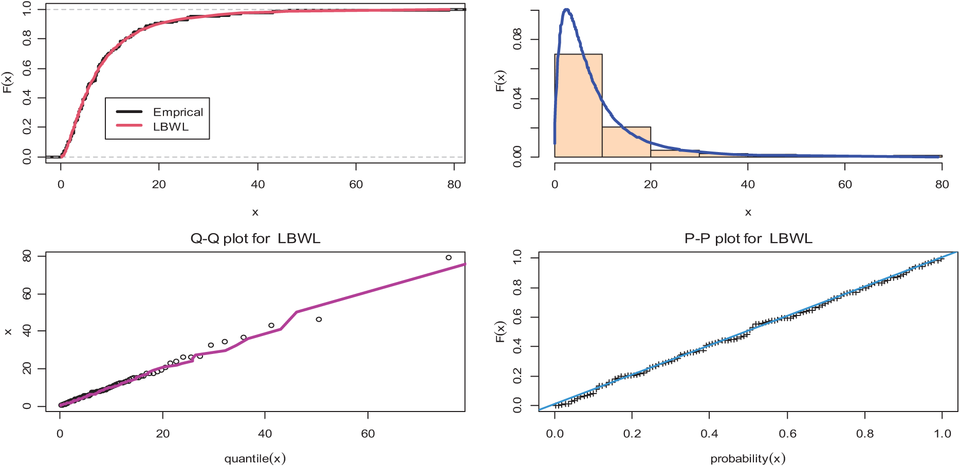
Figure 1: Plots of empirical cdf, histogram, PP-plots and QQ-plots for the LBWL distribution

7  Application to Real Data

In order to further demonstrate the performance of the proposed method, a real data set was used. The R-statistical programming language was used for computation. The dataset was an uncensored dataset consisting of the remission times (in months) of a random observation of 128 bladder cancer patients reported in [27]. The LBWL distribution was fitted to real data using the Kolmogorov-Smirnov goodness of the fit test. The estimated values of parameters were: θ^=4.325,λ^=10.974, and p = 0.9983. The empirical CDF, the histogram of the PDF, PP plots, and QQ plots are displayed in Fig. 1.

Based on the real data, the SS-PALT of the LBWL distribution under the PTIIC with binomial removals was considered. The ML and Bayesian estimates of parameters and accelerated factor were calculated. In addition, the ACIs for parameters and accelerated factor of the LBWL distribution at a different significant level for n = 70, β=8, and p = 0.75 were also calculated.

Tab. 5 presents the ML and Bayesian estimates of θ, λ, and β and their standard errors (SEs) at τ=9,β=8 and τ=9,β=15.

Table 5: ML, Bayesian estimates and their SEs based on SS-PALT under PTIIC data with binomial removals for real data

The history plots, approximate marginal posterior density, and MCMC convergence of θ, λ, and β are represented in Fig. 2.

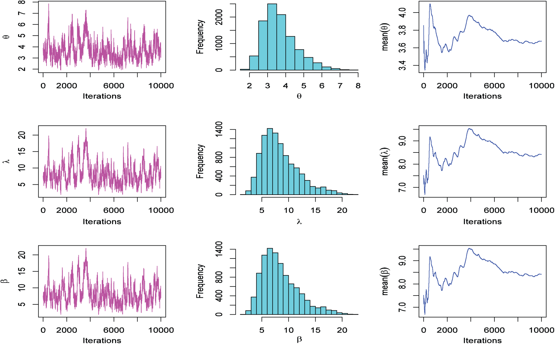
Figure 2: The MCMC plots for data based on SS-PALT under PTIIC data with binomial removals

The ACIs for parameters of the LBWL distribution based on the SS-PALT under the PTIIC data with binomial removals at a different level of significance for n = 70, β=8, and p = 0.75 are presented in Fig. 3.

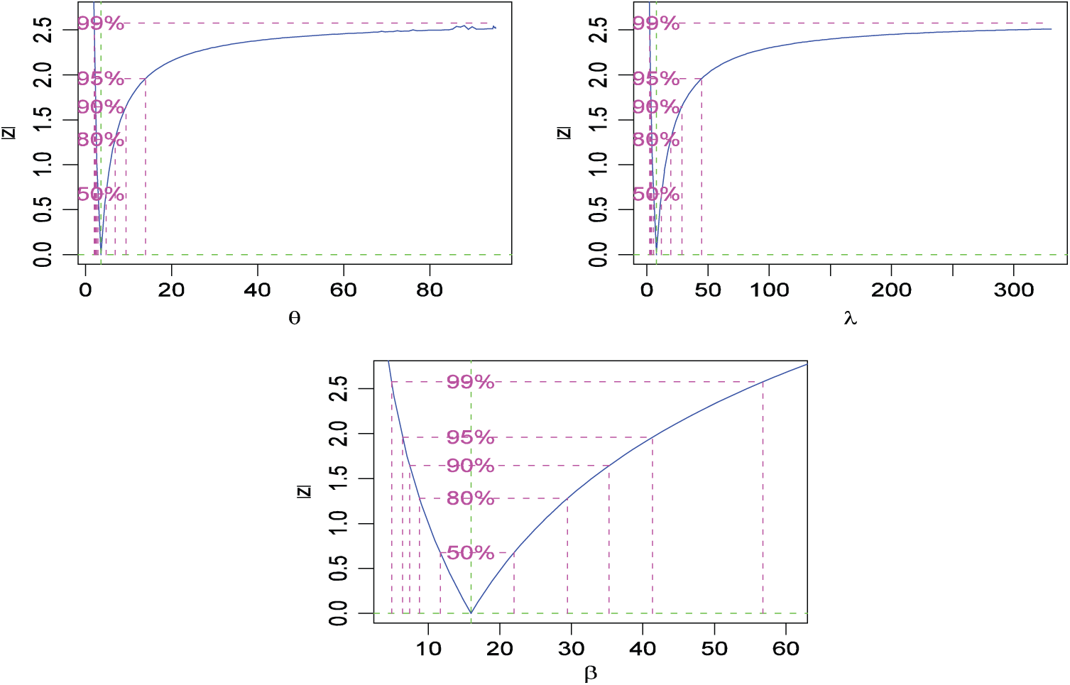
Figure 3: Plots of ACIs for SS-PALT under PTIIC data with binomial removals of real data

8  Conclusion

In this paper, the Bayesian and maximum likelihood estimation methods for the LBWL distribution are discussed based on SS-PALT using the PTIIC data with binomial removals. The approximate confidence intervals of the ML estimators of the model parameters are assessed based on the Fisher information matrix. In addition, the percentile bootstrap and bootstrap-t confidence intervals are determined. Moreover, the effects of sample size n, failure size m, and removal probability p on the accuracy of estimates are studied by simulation studies. The application of the proposed methods to real data is given for illustration purposes.

The simulation results show that, for fixed values of m and p, the performances of both estimation methods improve with n, and for fixed n and p, their performances improve with m, also for fixed n and m, their performances improve with p. Generally, the Bayesian estimates are better than the ML estimates in most situations. The lengths of the percentile bootstrap and bootstrap-t are smaller than those of the corresponding ACIs. For small sample sizes, Bootstrap- t CIs are better than the Bootstrap-p CIs in the sense of having smaller widths. However, the differences between the lengths of CIs using both methods decrease when sample sizes increase. In fact, the removal probability p is an important factor on the accuracy of the parameter estimates. When p is large, n–m of the n test units would be dropped out at the early stage of the life test.

As a future work, this study can be extended to explore the situation under type-I progressive censoring. Evaluation of the coverage probabilities can also be computed rather than the lengths of the CIs.

Acknowledgement: This project was funded by the Deanship of Scientific Research (DSR), at King Abdulaziz University, Jeddah, under Grant No. FP-190-42. The authors, therefore, thank DSR’s technical and financial support.

Funding Statement: This work was funded by the Deanship of Scientific Research (DSR), King Abdulaziz University, Jeddah, under Grant No. FP-190-42.

Conflicts of Interest: The authors declare that they have no conflicts of interest to report regarding the present study.

References

 1.  W. Nelson, Accelerated Life Testing: Statistical Models, Data Analysis and Test Plans. New York: John Wiley and Sons, 1990. [Google Scholar]

 2.  N. Balakrishnan, “Progressive censoring methodology: An appraisal (with discussions),” Test, vol. 16, pp. 211–296, 2007. [Google Scholar]

 3.  M. H. DeGroot and P. K. Goel, “Bayesian and optimal design in partially accelerated life testing,” Naval Research Logistics Quarterly, vol. 16, no. 2, pp. 223–235, 1979. [Google Scholar]

 4.  S. Bai and S. W. Chung, “Optimal design of partially accelerated life tests for the exponential distribution under type-I censoring,” IEEE Transactions on Reliability, vol. 41, no. 3, pp. 400–406, 1992. [Google Scholar]

 5.  H. M. Aly and A. A. Ismail, “Optimum simple time-step stress plans for partially accelerated life testing with censoring,” Far East Journal of Theoretical Statistics, vol. 24, no. 2, pp. 175–200, 2008. [Google Scholar]

 6.  A. M. Abd-Elfattah, A. S. Hassan and S. G. Nassr, “Estimation in step-stress partially accelerated life tests for the Burr Type XII distribution using type I censoring,” Statistical Methodology, vol. 5, no. 6, pp. 502–514, 2008. [Google Scholar]

 7.  P. W. Srivastava and N. Mittal, “Optimum step–stress partially accelerated life tests for truncated logistic distribution with censoring,” Applied Mathematical Modelling, vol. 34, no. 10, pp. 3166–3178, 2010. [Google Scholar]

 8.  A. S. Hassan and A. K. Thobety, “Optimal design of failure step stress partially accelerated life tests with Type II censored inverted Weibull data,” International Journal of Engineering Research and Applications, vol. 2, no. 3, pp. 3242–3253, 2012. [Google Scholar]

 9.  A. S. Hassan, “On the optimal design of failure step-stress partially accelerated life tests for exponentiated inverted Weibull with censoring,” Australian Journal of Basic and Applied Sciences, vol. 7, no. 1, pp. 97–104, 2013. [Google Scholar]

10. N. Balakrishnan and R. Aggarwala, Progressive Censoring: Theory, Methods, and Applications. Boston: Birkhauser, 2000. [Google Scholar]

11. A. Ismail and A. M. Sarhan, “Optimal design of step-stress life test with progressively type-II censored exponential data,” International Mathematical Forum, vol. 4, no. 40, pp. 1963–1976, 2009. [Google Scholar]

12. A. S. Hassan, M. Abd-Alla and H. G. A. El-Elaa, “Estimation in step stress partially accelerated life test for exponentiated Pareto distribution under progressive censoring with random removal,” Journal of Advances in Mathematics and Computer Science, vol. 7, no. 1, pp. 1–16, 2017. [Google Scholar]

13. E. M. Almetwaly and H. M. Almongy, “Estimation of the generalized power Weibull distribution parameters using progressive censoring schemes,” International Journal of Probability and Statistics, vol. 7, no. 2, pp. 51–61, 2018. [Google Scholar]

14. E. M. Almetwally and H. M. Almongy, “Maximum product spacing and Bayesian method for parameter estimation for generalized power Weibull distribution under censoring scheme,” Journal of Data Science, vol. 17, no. 2, pp. 407–444, 2019. [Google Scholar]

15. E. S. A. El-Sherpieny, E. M. Almetwally and H. Z. Muhammed, “Progressive type-II hybrid censored schemes based on maximum product spacing with application to power Lomax distribution,” Physica A: Statistical Mechanics and its Applications, vol. 553, no. 1, pp. 124251, 2020. [Google Scholar]

16. A. Atkinson and A. Harrison, Distribution of Personal Wealth in Britain. Cambridge: Cambridge University Press, 1978. [Google Scholar]

17. A. A. Balkema and L. de Hann, “Residual life time at great age,” Annals of Probability, vol. 2, no. 5, pp. 972–804, 1974. [Google Scholar]

18. A. S. Hassan and A. S. Al-Ghamdi, “Optimum step stress accelerated life testing for Lomax distribution,” Journal of Applied Sciences Research, vol. 5, no. 12, pp. 2153–2164, 2009. [Google Scholar]

19. A. S. Hassan, S. M. Assar and A. Shelbaia, “Optimum step stress accelerated life test plan for Lomax distribution with an adaptive type-II progressive hybrid censoring,” British Journal of Mathematics & Computer Science, vol. 13, no. 2, pp. 1–19, 2016. [Google Scholar]

20. A. A. H. Ahmadini, A. N. Zaki, A. S. Hassan and S. S. Alshqaq, “Bayesian inference of dynamic cumulative residual entropy from Parto II distribution with application to covid 19,” AIM Mathematics, vol. 6, no. 3, pp. 2196–2216, 2020. [Google Scholar]

21. A. S. Hassan and A. N. Zaki, “Entropy Bayesian estimation for Lomax distribution based on record,” Thailand Statistician, vol. 19, no. 1, pp. 96–115, 2021. [Google Scholar]

22. A. Ahmad, S. P. Ahmad and A. Ahmed, “Length-biased weighted Lomax distribution: Statistical properties and application,” Pakistan Journal of Statistics and Operation Research, vol. 12, no. 2, pp. 245–255, 2016. [Google Scholar]

23. H. Karimi and P. Nasiri, “Estimation parameter of R = P(Y < X) for length-biased weighted Lomax distributions in the presence of outliers,” Mathematical and Computational Applications, vol. 23, no. 9, pp. 1–9, 2018. [Google Scholar]

24. S. Dey, S. Singh, Y. M. Tripathi and A. Asgharzadeh, “Estimation and prediction for a progressively censored generalized inverted exponential distribution,” Statistical Methodology, vol. 32, no. 1, pp. 185–202, 2016. [Google Scholar]

25. N. Metropolis, A. W. Rosenbluth, M. N. Rosenbluth, A. H. Teller and E. Teller, “Equation of state calculations by fast computing machines,” Journal of Chemical Physics, vol. 21, no. 6, pp. 1087–1092, 1953. [Google Scholar]

26. W. K. Hastings, “Monte Carlo sampling methods using Markov chains and their applications,” Biometrika, vol. 57, no. 1, pp. 97–109, 1970. [Google Scholar]

27. E. T. Lee and J. Wang, Statistical Methods for Survival Data Analysis, Hoboken, New Jersey, United States: John Wiley and Sons, 2003. [Google Scholar]

This work is licensed under a Creative Commons Attribution 4.0 International License, which permits unrestricted use, distribution, and reproduction in any medium, provided the original work is properly cited.