DOI:10.32604/cmc.2021.014840
| Computers, Materials & Continua DOI:10.32604/cmc.2021.014840 | |
| Article |
A New Hybrid Feature Selection Method Using T-test and Fitness Function
1Department of Computer Science, Faculty of Science, University of Baghdad, Baghdad, Iraq
2Faculty of Computer Science, Technology University, Baghdad, Iraq
3Department of Computer Science, Al-Turath University College, Baghdad, Iraq
*Corresponding Author: Husam Ali Abdulmohsin. Email: husam.a@sc.uobaghdad.edu.iq
Received: 21 October 2020; Accepted: 08 March 2021
Abstract: Feature selection (FS) (or feature dimensional reduction, or feature optimization) is an essential process in pattern recognition and machine learning because of its enhanced classification speed and accuracy and reduced system complexity. FS reduces the number of features extracted in the feature extraction phase by reducing highly correlated features, retaining features with high information gain, and removing features with no weights in classification. In this work, an FS filter-type statistical method is designed and implemented, utilizing a t-test to decrease the convergence between feature subsets by calculating the quality of performance value (QoPV). The approach utilizes the well-designed fitness function to calculate the strength of recognition value (SoRV). The two values are used to rank all features according to the final weight (FW) calculated for each feature subset using a function that prioritizes feature subsets with high SoRV values. An FW is assigned to each feature subset, and those with FWs less than a predefined threshold are removed from the feature subset domain. Experiments are implemented on three datasets: Ryerson Audio-Visual Database of Emotional Speech and Song, Berlin, and Surrey Audio-Visual Expressed Emotion. The performance of the F-test and F-score FS methods are compared to those of the proposed method. Tests are also conducted on a system before and after deploying the FS methods. Results demonstrate the comparative efficiency of the proposed method. The complexity of the system is calculated based on the time overhead required before and after FS. Results show that the proposed method can reduce system complexity.
Keywords: Feature selection; dimensional reduction; feature optimization; pattern recognition; classification; t-test
Feature selection (FS) is a preprocessing step in machine learning [1] that enhances classification accuracy. It is the process of feature subset selection from a pool of correlated features for use in modeling construction [2]. This work aims to decrease the high correlation between features that causes numerous drawbacks, including a failure to gain additional information and improve system performance, an increase in computational requirements during training, and instability for some systems [3].
FS algorithms have goals such as to consume less time for learning, reduce the dimensionality and complexity of systems, reduce correlation and time consumption, and increase system accuracy [4]. FS methods have been said to decrease the data burden and avoid overfitting [5]. FS methods are considered a combination of search methods that produce feature subsets scored by evaluation measures. The simplest FS method tests all possible subsets and finds the best accuracy. Although, the approach is time-consuming, it can identify the feature subset with the highest clustering accuracy. An enhanced version of the simplest FS method was presented, and a parallel FS method was proposed, in which each feature subset is tested individually and a scoring function measures the relevance between features [6].
Many FS methods have been developed, which can be categorized according to multiple topologies. This work is concerned with statistics; hence we classify FS methods according to the distance measures used to evaluate subsets. Distance measures distinguish redundant or irrelevant features from the main pool, and four types of FS methods can be identified according to their distance measures [7].
• Wrapper methods assign scoring values to each feature subset after training and testing the model. This requires considerable time, but it obtains the subset with the highest accuracy. The three wrapped FS methods of optimization selection, sequential backward selection, and sequential forward selection (SFS), based on ensemble algorithms called bagging and AdaBoost, were used [8]. Subset evaluations were performed using naïve Bayes and decision tree classifiers. Thirteen datasets with different numbers of attributes and dimensions were obtained from the UCI Machine Learning Repository. The search technique using SFS based on the bagging algorithm and using decision trees gained the results with the best average accuracy (89.60%).
• Filter methods measure the relevance of features through univariate statistics. In tests of 32 FS methods on four gene expression datasets, it was found that filter methods outperform wrapper and embedded methods [9].
• Embedded methods differ in terms of learning and interaction of the FS phase. Unlike filter methods, wrapper methods utilize learning to measure the quality of several feature subsets without knowledge of the structure of the classification or regression method used. Therefore, these methods can work with any learning machine. Embedded methods do not separate the learning and FS phases, and the structure of the class of functions under consideration plays a crucial role. An example is the measurement of the value of a feature using a bound that is valid for support vector machine (SVM) only and not for the decision tree method [10].
• Hybrid methods utilize two or more FS methods. An efficient hybrid method consisting of principal component analysis and ReliefF was proposed [11]. Ten benchmark disease datasets were used for testing. The approach eliminated 50% of the irrelevant and redundant features from the dataset and significantly reduced the computation time.
FS methods employ strategies based on the types of feature subsets: redundant and weakly relevant, weakly relevant and non-redundant, noisy and irrelevant, and strongly relevant [12]. The current study aims to remove redundant and strongly correlated features by deploying a t-test, and to find coupled features with high dependency by deploying a fitness function. Although FS puts an enormous burden on the system performance pool, FS in pattern recognition systems is rarely avoided.
FS Methods main concepts:
• FS methods are employed either to reduce system complexity or increase accuracy. A study in 2006 employed two FS algorithms, the t-test method to filter irrelevant and noisy genes and kernel partial least squares (KPLS) to extract features with high information content [13]. It was found that neither method achieved high classification results. FS methods do not necessarily increase the classification accuracy of pattern recognition systems. They can remove all relevant features without conflict between the removed features [14,15].
• There is no superior FS method. Research has shown that no specific group of FS filter methods outperforms other groups constantly, but observations have indicated that certain groups of FS filter methods perform best with many datasets [3,16]. Many FS methods have been used in pattern recognition research and in different scientific fields, with largely varying results. Furthermore, each FS filter method performs differently with respect to specific types of datasets, and this is called FS algorithm instability [17].
One drawback of statistical FS algorithms is that they do not consider the dependency of features on others; statistical FS algorithms can eliminate a feature whose absence negatively affects the performance of another selected feature because of their strong interrelationship [17]. This work avoids this drawback by calculating the dependency of each feature on other features. State-of-the-art methods make decisions on the removal of highly correlated features without a basis in proper measurement. Two highly correlated features can be powerful in classifying two different attributes. Thus, to remove one can severely affect classification. To avoid this, we calculate the strength of recognition value (SoRV) and assign it a high weight through an exponential function. The proposed method outperforms the state-of-the-art through a fitness function that calculates SoRV for each feature and subset feature (pair of features). To remove a feature can also affect the performance of another feature. To avoid this, we group features in subsets of pairs to calculate the degree of dependence between each feature and all other features.
In the proposed method, there is a maximum of two features in each tested subset. To use a combination of three or more features in each feature subset will exponentially increase the time consumption, and to reach the optimal solution will take months. Nevertheless, subsets of two features provide good results in a reasonable amount of time. Hence, we fix the number of features per subset to two. We focus on statistical filter FS methods because of their stability, scalability, and minimal time consumption.
The remainder of this paper is organized as follows. Section 2 explores some recent FS methods that utilize the t-test and feature ranking approaches. Section 3 explains the proposed methodology. Section 4 shows the experimental setup and the results gained through this work. Section 5 discusses our conclusions and trends for future work.
The t-test is deployed in many fields to measure the convergence relevance between samples. A proposed gene selection method utilized two FS methods, the t-test to remove noisy and irrelevant genes and KPLS to select features with noticeable information content [13]. Three datasets were used in a performance experiment, and the results showed that neither method yielded satisfactory results. A modified hybrid ranking t-test measure was applied to genotype HapMap data [18]. Each single nucleotide polymorphism (SNP) was ranked relative to other importance feature measures, such as F-statistics and the informativeness for assignment. The highest ranked SNPs in different groups in different numbers were selected as the input to a class SVM to find the best classification accuracy achieved by a specific feature subset. A two-class FS algorithm utilizing the Student’s t-test was used to extract statistically relevant features, and the  -norm SVM and recursive feature elimination were used to determine the patients at risk of cancer spreading to their lymph nodes [19]. A proposed FS method used the Student’s t-test to measure the term frequency distribution diversity between one category and the entire dataset [20]. An FS approach based on the nested genetic algorithm (GA) utilized filter and wrapper FS methods [21]. For the filter FS, a t-test was used to rank the features according to convergence and redundancy. A nested neural network and SVM were used as the wrapper FS technique. A t-test was utilized to compare outcome measures pre- and post-ablation through an intraprocedural 18F-fluorodeoxyglucose positron emission tomography (PET) scan assessment before and after PET/contrast-enhanced guided microwave ablation [22]. A fatigue characteristic parameter optimization selection algorithm utilized the classification performance of an SVM as an evaluation criterion and applied the sequential forward floating selection algorithm as a search strategy [23]. The algorithm aimed to reach the optimal feature subset of fatigue motion by reducing the dimensionality of the domain set of fatigue feature parameters. Based on the t-test analysis of variance method, the algorithm was used to analyze the influence of individual athlete differences and fatigue exercises on sports behavior and eye movement characteristics.
A filtered FS method is proposed to improve the emotion classification accuracy of the datasets deployed in this work. These are the Ryerson Audio-Visual Database of Emotional Speech and Song (RAVDESS), Berlin (Emo-DB), and Surrey Audio-Visual Expressed Emotion (SAVEE). The method uses the minimum number of features to achieve the highest accuracy in the least time.
The structure of the extracted features from each dataset is shown in Tab. 1. We explain the structure of features extracted from the RAVDESS dataset as an example. First, 2,186 features are extracted from each of the 1,440 audio wave file samples. The same number is extracted from Emo-DB and SAVEE.
Table 1: Structure of features extracted
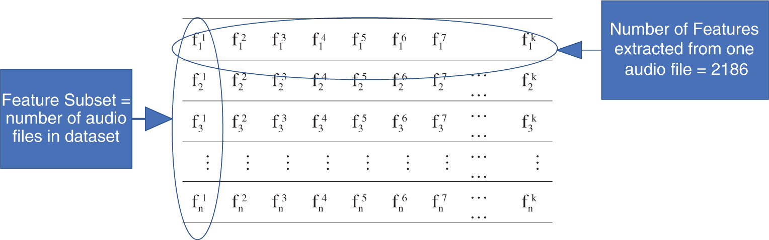
The number of features is k, as is the number of feature subsets. n is the number of samples in each feature subset, represented as (fji, fj+1i, fj+2i,…, fni), where n = 1,440 for RAVDESS, n = 553 for Emo-DB, and n = 480 for SAVEE. The feature number in a feature subset is denoted by i, and j is the sample number. Sections 3.1–3.3 discuss the procedures of the proposed FS method.
The t-test value is calculated between each subset and all other subsets through Eq. (1):
where k is the number of feature subsets, n is the number of samples in each feature subset; i = 1,…, k − 1, m = 1,…, n, and j = i + 1,…, k, to avoid calculating the quality of performance value (QoPV) for the same pair of feature subsets. The QoPV is obtained by calculating the t-test value between subset i and all other subsets. The QoPV for a subset decreases each time the t-test value is 0; otherwise, it increases. After calculating the QoPV of each feature subset with respect to all other subsets, the feature subsets are ranked according to their QoPVs in descending order.
This work uses a two-sample t-test, i.e., the so-called independent t-test, because the two groups of features being tested come from different features. The formula of the t-test function is shown in Eq. (2):
where x1 and x2 are the means of the two feature subsets being compared, as shown in Eq. (1); S2 is the pooled standard error of the two subsets; and fe1 and fe2 are the numbers of samples in the two subsets and are equal. The t-test indicates significant differences between pairs of feature subsets. A large t-test value indicates that the difference between the means of two groups is higher than the pooled standard error of the two feature subsets [24]. Thus, the higher the t-test value the better the results. Feature subsets with low t-test values must be removed because of the great similarity of their values to those of other feature subsets. However, the final decision is not made at this step, because a feature subset with a low QoPV might have a high SoRV. In case of a high SoRV, a subset may have a final weight (FW) higher than those of other feature subsets with a high QoPV. This reflects the novel idea of our work.
The SoRV for each subset i is obtained using the neural network-based fitness function. The SoRV is calculated through pairs of subsets to observe the classification effect of each feature subset i on all other feature subsets through Eq. (3):
where k is the number of feature subsets, n is the number of samples in each feature subset, i = 1,…, k − 1, m = 1,…, n, and j = i + 1,…, k. After performing several experiments, the percentage of 37% achieves the highest performance for the tested features.
3.3 Final Weight (FW) Calculation
Several experiments show that SoRV is more important than QoPV. Specifically, SoRV indicates the power of recognition for each feature subset, whereas QoPV indicates the convergence of the feature subset with respect to other feature subsets. Nevertheless, we need QoPV to determine the degree of convergence of each feature subset. Thus, we use Eq. (4) to assign a higher weight to SoRV than to QoPV.
Using Eq. (4), we calculate FW for all feature subsets i, i = 1, 2,…, k, where k is the number of feature subsets. All feature subsets are sorted in descending order of their FWs. In the final phase of the proposed method, we select features that will gain the highest emotion recognition accuracy. The number of features selected at the beginning is 20, because lengths less than this result in low classification accuracy. Thus the 20 features with the highest FW values are selected and evaluated through the fitness neural network function used in Eq. (3). Other features are added according to the sorted list of FWs. The FS process stops when emotion recognition accuracy stops increasing and adding other features does not improve it. The final numbers of features selected by the proposed method from the 2,186 features extracted from the RAVDESS, Emo-DB, and SAVEE datasets are 333, 247, and 270, respectively. The pseudocode of the proposed method is shown in Fig. 1.
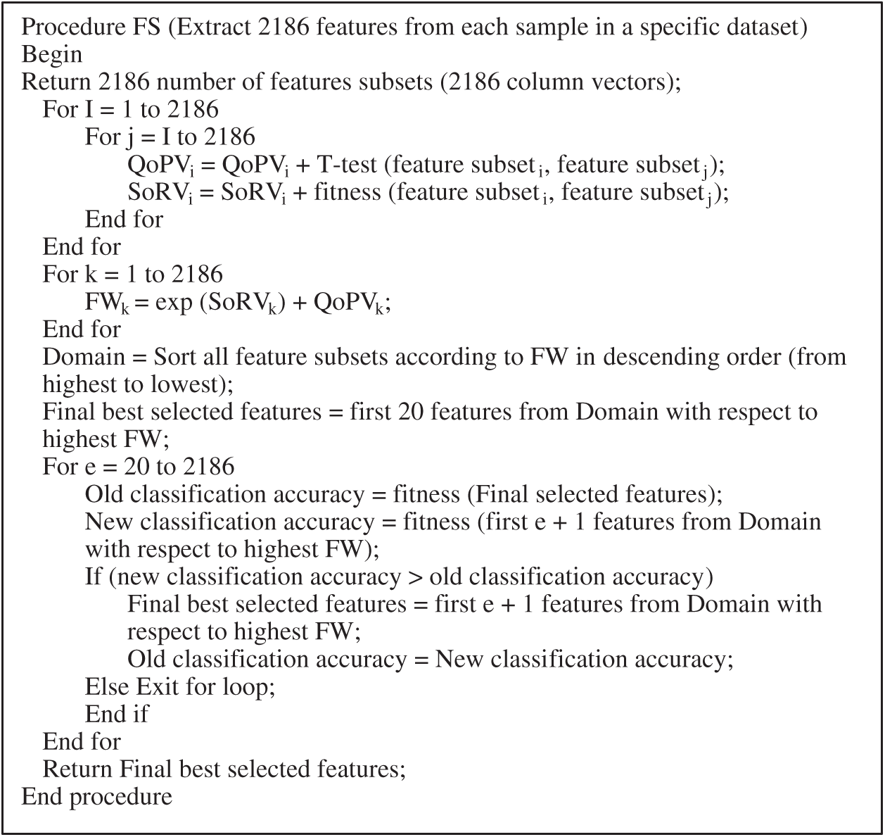
Figure 1: Pseudocode of proposed FS method
Section 4.1 discusses the experimental setup, Section 4.2 describes the datasets used in the experiments, and Section 4.3 explains the experimental results.
All audio files were preprocessed prior to feature extraction. Silent parts at the beginning and end of each file were removed, data were normalized to the interval (0, 100), and files were grouped according to the emotions they represented. The number of features extracted from each audio file was 2,186. Audio file samples were selected randomly for evaluation, and 70%, 15%, and 15% of the samples of each dataset were selected for training, validation, and testing, respectively. To evaluate the proposed FS method, we used a one-layer, 10-node neural network classifier. Feature extraction was applied to each of the three datasets before application of the proposed method.
The datasets used in this work were selected through an online search according to the following criteria.
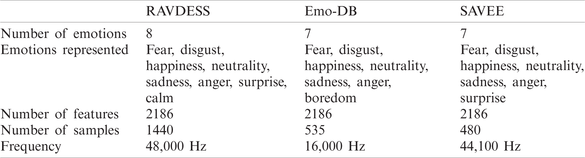
• This work proposes an FS method for use in speech emotion recognition. Thus, the most important criteria are the emotions represented in a dataset. Selected datasets should represent the six basic emotions of fear, disgust, happiness, sadness, anger, and surprise, according to Paul Ekman’s definition [25]. The three selected datasets intersect to represent fear, disgust, happiness, neutrality, sadness, and anger, which include five of the basic emotions. The RAVDESS dataset represents eight emotions through 1440 audio files, and Emo-DB and SAVEE represent seven emotions through 535 and 480 audio files, respectively.
• The selected datasets should be recorded at different frequencies to test the proposed method. The RAVDESS, Emo-DB, and SAVEE datasets were recorded at 48,000, 16,000, and 44,100 Hz, respectively, as shown in Tab. 2.
• Datasets should show gender balance; this criterion was met in this work.
The same feature extraction process was implemented on each of the datasets, and 2,186 features were proposed for each audio file. These were established by a predefined feature extraction method that utilizes 15 features: entropy, zero crossing (ZC), deviation of ZC, energy, deviation of energy, harmonic ratio, Fourier function, Haar, MATLAB fitness function, pitch function, loudness function, Gammatone Cepstrum Coefficient according to time and frequency, and the MFCC function according to time and frequency. The standard deviation (SD) of these features was calculated using 14 degrees on either side of the mean (i.e., 0.25, 0.5, 0.75, 1, 1.25, 1.5, 1.75, 2, 2.25, 2.5, 2.75, 3, 3.5, and 4). All experiments were implemented separately on each dataset.
We discuss the experimental results. The performance efficiency of the proposed FS method is evaluated through a neural network classifier. Three emotional datasets are used in the evaluation process, as shown in Tab. 2. The accuracy of the classifier is calculated using confusion matrices and receiver operating characteristics (ROCs). The confusion matrices represent emotions as numbers.
Table 2: Datasets used in this work
The confusion matrices related to the RAVDESS dataset show the following emotions from left to right, which we denote as 1 to 8, in the following order: neutrality, calm, happiness, sadness, anger, fear, disgust, and surprise. The confusion matrices related to the Emo-DB dataset show the following emotions from left to right, denoted as 1 to 7, in this order: fear, disgust, happiness, boredom, neutrality, sadness, and anger. The confusion matrices related to the SAVEE dataset show the following emotions from left to right, denoted as 1 to 7, in the following order: anger, disgust, fear, happiness, sadness, surprise, and neutrality. The ROC line chart is one of the best techniques for testing the results of a classification system. It is a two-dimensional line chart; the x-axis shows the false-positive rate (FPR), and the y-axis shows the true-positive rate (TPR). The ROC shows the relationship between sensitivity and specificity. It is generated by plotting the TPR value against the FPR value. TPR is the ratio of cases correctly predicted as positive (i.e., true positive, or TP) to all positive cases (i.e., false negative, or FN), as shown in Eq. (5).
The FPR is the ratio of cases incorrectly predicted as positive (i.e., false positive, or FP) to all negative cases (i.e., true negative, or TN), as shown in Eq. (6).
The ROC curve is a compromise between TPR (or sensitivity) and (1 – FPR) (or specificity). The degree to which the curves are tangent to the top-left corner of the ROC line chart indicates the performance of the classification process in making correct predictions. The closer the curve is to the 45° diagonal of the ROC space, the less accurate the classification is because of incorrect predictions [26]. The greatest advantage of the ROC in evaluating classifiers is that it does not depend on class distribution, but rather depends on classifier prediction. The results achieved from our experiments are presented in Tab. 3, which compares the proposed FS method to the widely used F-test and F-score methods. Tab. 3 shows that the proposed FS method achieves the highest classification accuracy among these methods.
Tab. 3 and Figs. 2–4 present the accuracy classification results for the three datasets before deploying the FS methods (utilizing all 2,186 features), which are 93.05%, 95%, and 97.2% for the RAVDESS, Emo-DB, and SAVEE datasets, respectively.
Table 3: Accuracy percentages achieved by implementing the experiments with and without the FS method
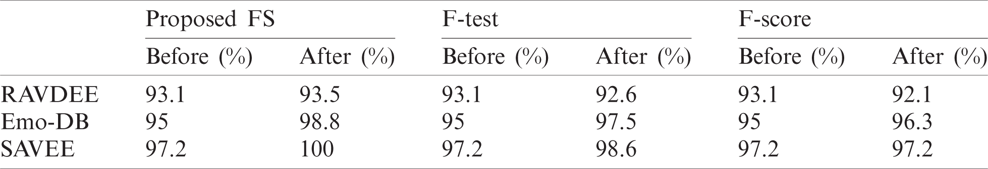
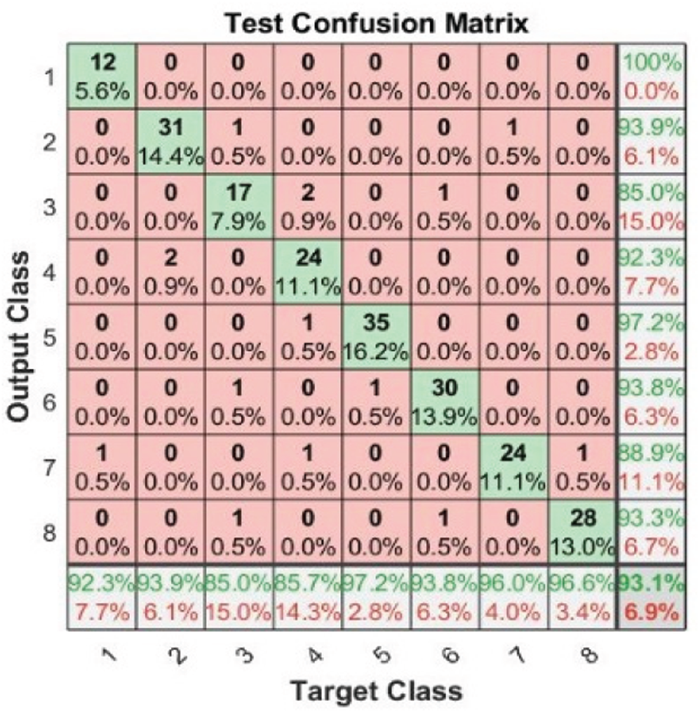
Figure 2: Test confusion matrix before applying FS methods on RAVDESS
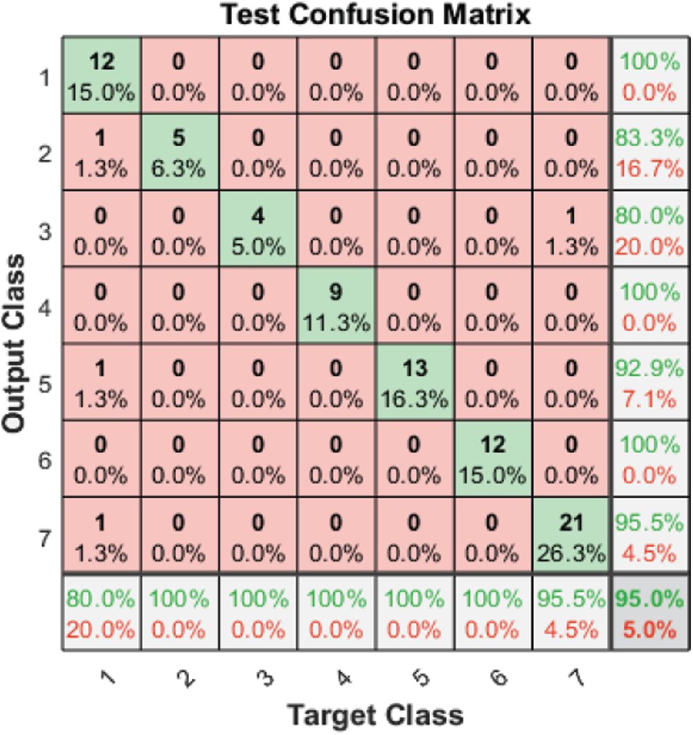
Figure 3: Test confusion matrix before applying FS methods on Emo-DB

Figure 4: Test confusion matrix before applying FS methods on the SAVEE
Figs. 5–7 show the classification accuracies after running the three FS methods on the RAVDESS, Emo-DB, and SAVEE datasets, respectively. The highest classification accuracy gained in this work was through running the proposed FS method on all three datasets. The highest classification accuracies achieved from running the proposed, F-test, and F-score FS methods on the RAVDESS dataset are 93.5%, 92.6%, and 92.1%, respectively, as shown in Figs. 5a–5c, and Tab. 3. These values are lower than those obtained without using FS methods because many of the emotions represented in RAVDESS audio samples are similar and are thus difficult to distinguish. The same is true of realistic datasets. This similarity between audio samples produces similarity in the extracted features; hence the proposed, F-test, and F-score FS methods yield poor outcomes.
Tab. 3 and Fig. 6 show the classification accuracies after deploying the three FS methods on the Emo-DB dataset. The proposed FS method gains the highest classification accuracy. The F-test and F-score FS methods achieve accuracies of 97.5% and 96.3%, respectively. As observed in the confusion matrices, each FS method affects the recognition of a certain emotion. The proposed method affects the recognition of the happy emotion. The F-test FS method affects the recognition of fear and anger. The F-score FS method affects the recognition of boredom.
Tab. 3 and Fig. 7 show the classification accuracies after deploying the three FS methods on the SAVEE dataset. We notice that the proposed FS method gains the highest accuracy among all compared methods. Specifically, the proposed FS method gains 100% classification accuracy, compared to 98.6% and 97.2%, respectively, for the F-test and F-score methods. The F-score FS method achieves no improvement to the classification accuracy.
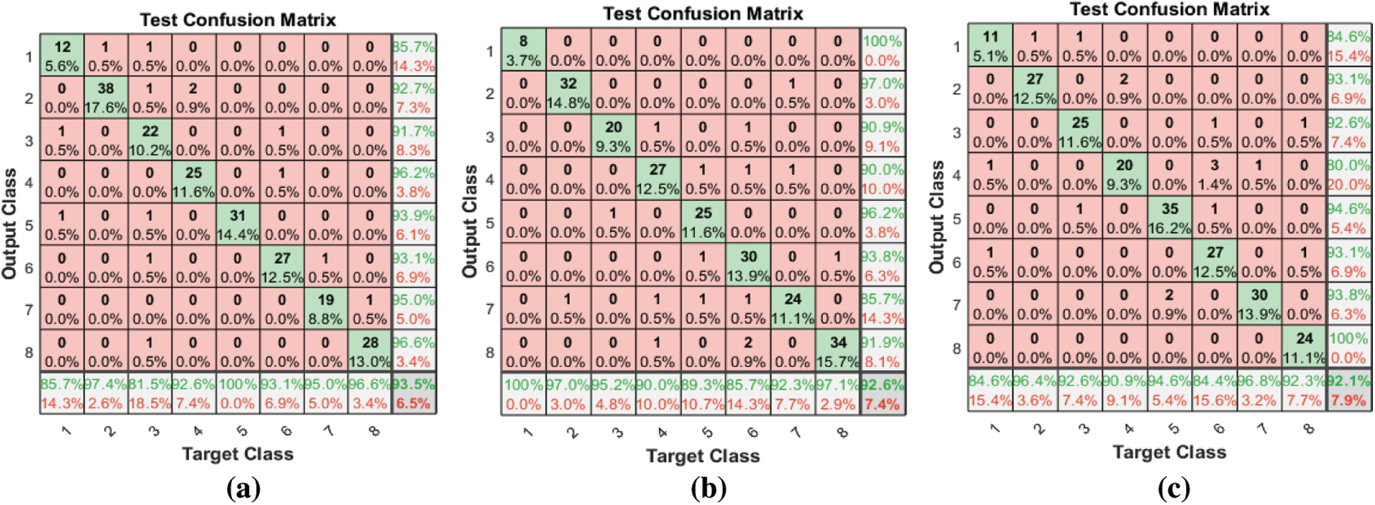
Figure 5: (a) Test confusion matrix after applying the proposed FS method on RAVDESS (b) Test confusion matrix after applying F-test FS method on RAVDESS (c) Test confusion matrix after applying F-score FS method on RAVDESS
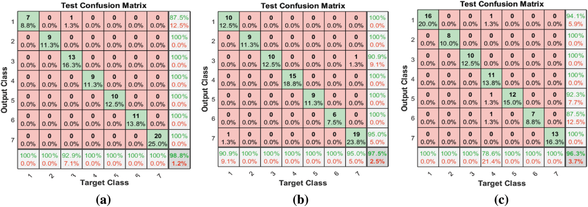
Figure 6: (a) Test confusion matrix after applying the proposed FS method on Emo-DB (b) Test confusion matrix after applying F-test on the Emo-DB (c) Test confusion matrix after applying the F-score on Emo-DB
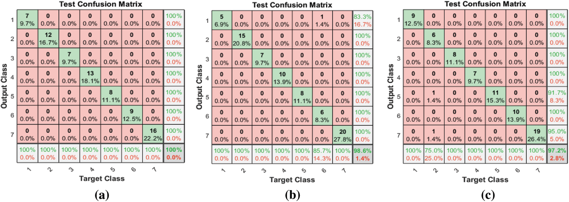
Figure 7: (a) Test confusion matrix after applying the proposed FS method on SAVEE (b) Test confusion matrix after applying F-test on SAVEE (c) Test confusion matrix after applying F-score on SAVEE
All the results shown in the confusion matrices are described by the legend charts shown in Fig. 8. The results highlight the superiority of the proposed FS method over the F-test and F-score FS methods.
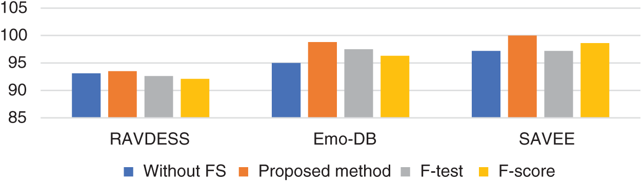
Figure 8: The legend chart of the results gained in this work on the three datasets utilized
As mentioned in Section 4.2, the results are also analyzed using the ROC line chart. Figs. 9–11 show the ROC curves for the classification processes on the RAVDESS, Emo-DB, and SAVEE datasets, respectively, before deploying the FS methods. Through the confusion matrices, we show numerically the superior performance of the proposed FS method over the other two FS methods. Through the ROC line charts, we show visually that the proposed method outperforms the F-test and F-score FS methods.
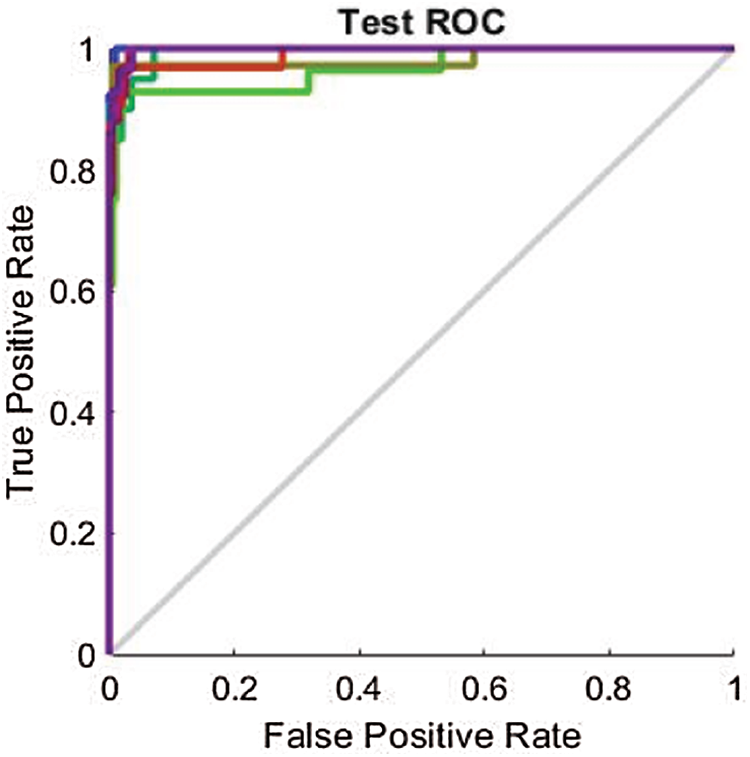
Figure 9: Test ROC line chart before applying FS methods on RAVDESS
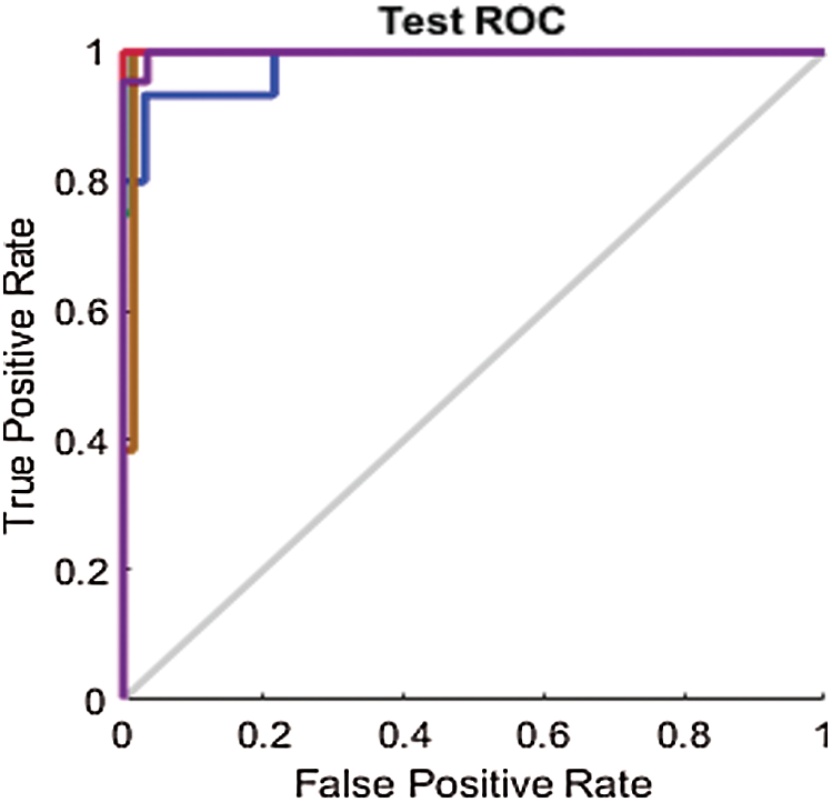
Figure 10: Test ROC line chart before applying FS methods on Berlin
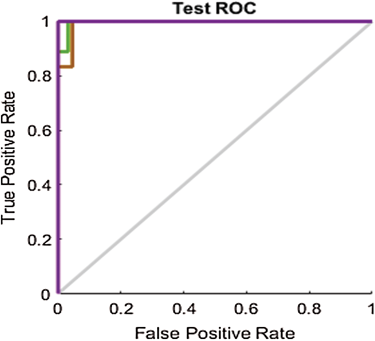
Figure 11: Test ROC line chart before applying FS methods on SAVEE
Through a visual comparison of the ROC curves in Fig. 9 and the ROC curves in Fig. 12, we notice that all the ROC curves in Figs. 12a–12c are farther from the top-left corner than those in Fig. 9. This demonstrates the failure of FS methods to prove the results, while the proposed method attained the highest results. The ROC curves in Fig. 12a, are closer to the top-left corner than those in Figs. 12b and 12c. This demonstrates that the optimum performance is achieved by the proposed FS method.
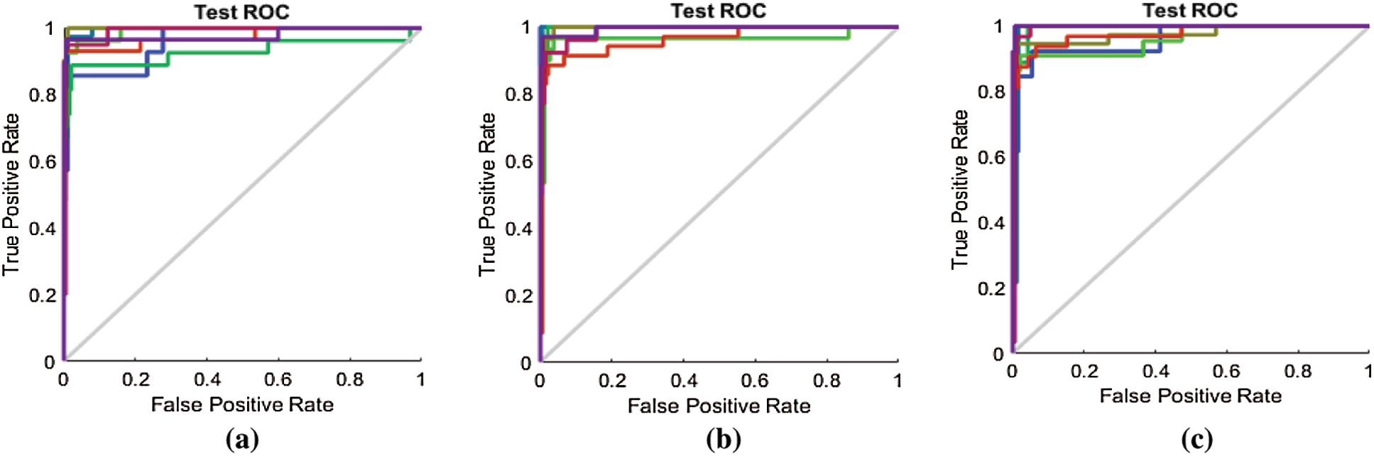
Figure 12: (a) ROC line chart after applying the proposed FS method on RAVDESS (b) ROC line chart after applying F-test on RAVDESS (c) ROC line chart after applying F-score on RAVDESS
We similarly compare the ROC curves in Fig. 10 with those in Figs. 13a–13c for the Emo-DB dataset.
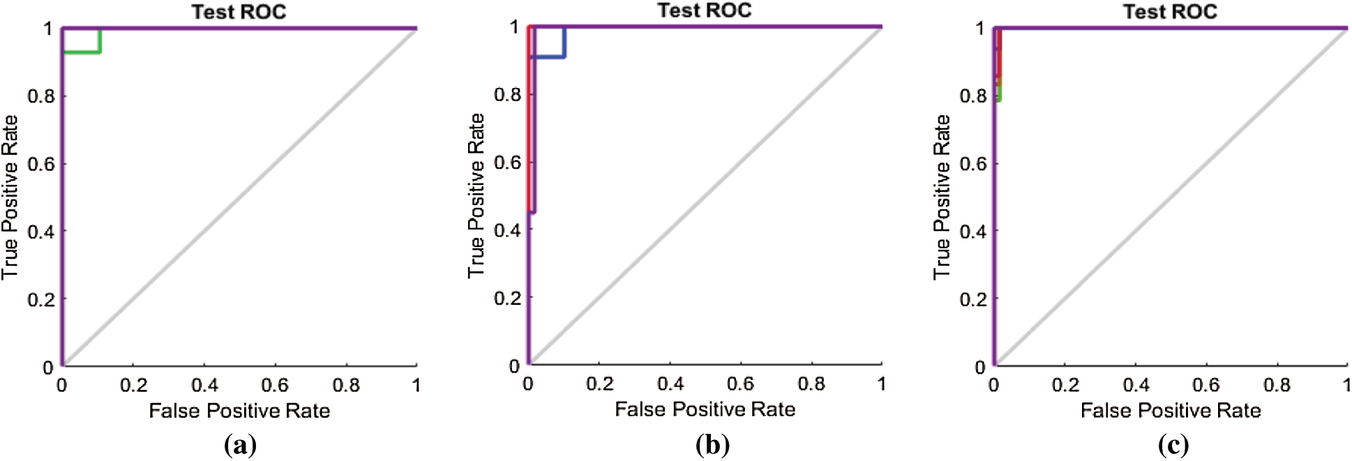
Figure 13: (a) ROC line chart after applying the proposed FS method on Emo-DB (b) ROC line chart after applying F-test on Emo-DB (c) ROC line chart after applying F-score on Emo-DB
The ROC curves in Fig. 11 are also compared with those in Figs. 14a–14c for the SAVEE dataset. All the curves in the ROC line chart shown in Fig. 14a pass through the top-left corner of the ROC. Hence the emotions represented in the SAVEE dataset are recognized using the proposed FS method, with 100% accuracy.
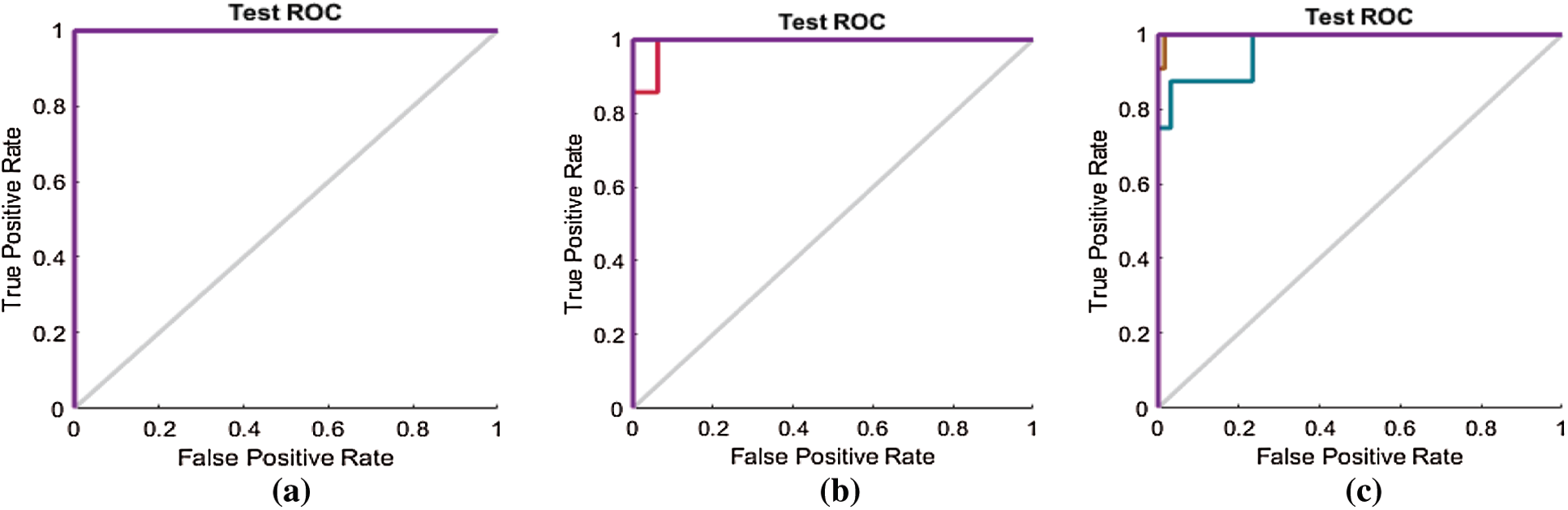
Figure 14: (a) ROC line chart after applying the proposed FS method on SAVEE (b) ROC line chart after applying F-test on SAVEE (c) ROC line chart after applying F-score on SAVEE
Time consumption is one of the most important factors in classification. Thus, for the proposed FS method, we prioritize time consumption. The proposed FS method performs well in terms of time consumption after decreasing the number of features. We observe in Figs. 15–17 that 2,186 features are used as input to the 10-node single-layer neural network.
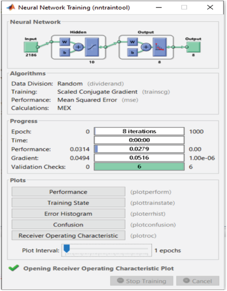
Figure 15: NN training window before applying FS methods on RAVDESS
For the RAVDESS dataset, eight epochs are needed to achieve 93.1% classification accuracy without using any FS method (Fig. 15). For the Emo-DB dataset, 67 epochs are needed to achieve 95% classification accuracy (Fig. 16). For the SAVEE dataset, six epochs are needed to achieve 97.2% classification accuracy (Fig. 17). Tab. 4 compares the numbers of epochs needed to classify the emotions in the datasets before deploying the FS methods for RAVDESS, Emo-DB, and SAVEE, respectively (Figs. 15–17), and similarly after deploying the FS methods (Figs. 18–20).
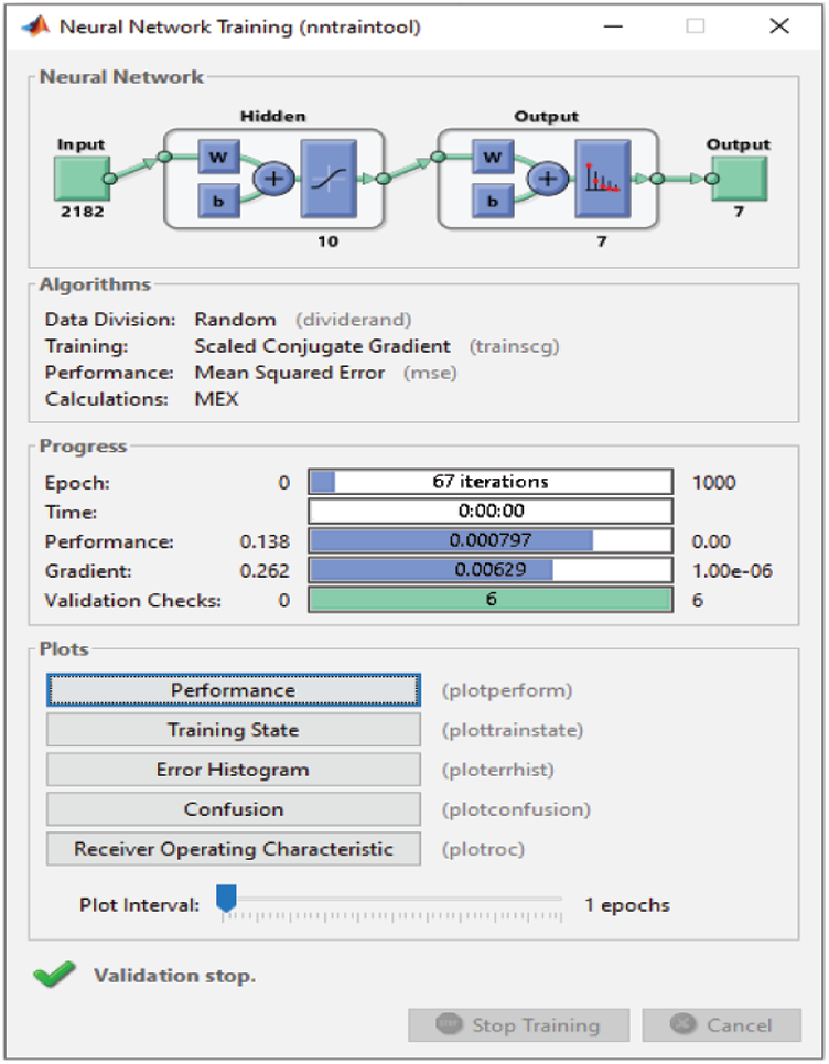
Figure 16: NN training window before applying FS methods on Emo-DB
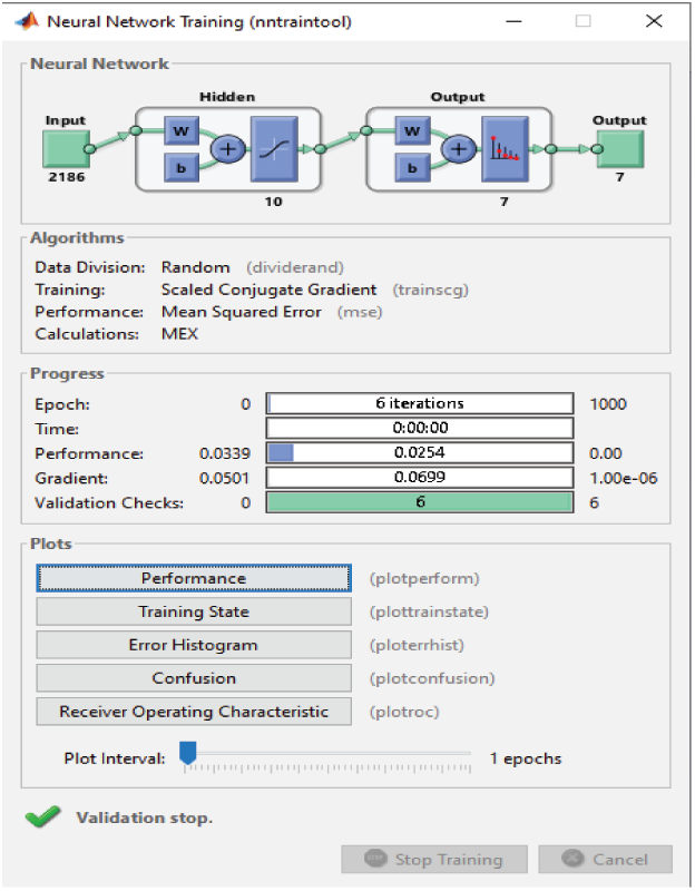
Figure 17: NN training window before applying FS methods on SAVEEE
When the proposed FS, F-test, and F-score FS methods are applied, classification takes 6 and 7 epochs, respectively (Fig. 18). Thus, the three FS methods have adequate classification times, but the proposed FS method is faster than the other two. When the proposed FS, F-test, and F-score FS methods are applied on the Emo-DB dataset, the classification process takes 9, 6, and 8 epochs, respectively (Fig. 19). Thus, the three FS methods have adequate classification times, and the F-test FS method is faster than the other two. Although the F-test FS method achieves the fastest time, its classification accuracy is 1.3% less than that of the proposed FS method.
Table 4: Time required to implement the experiments with and without the FS methods
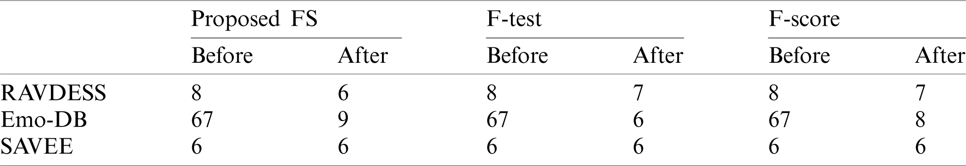
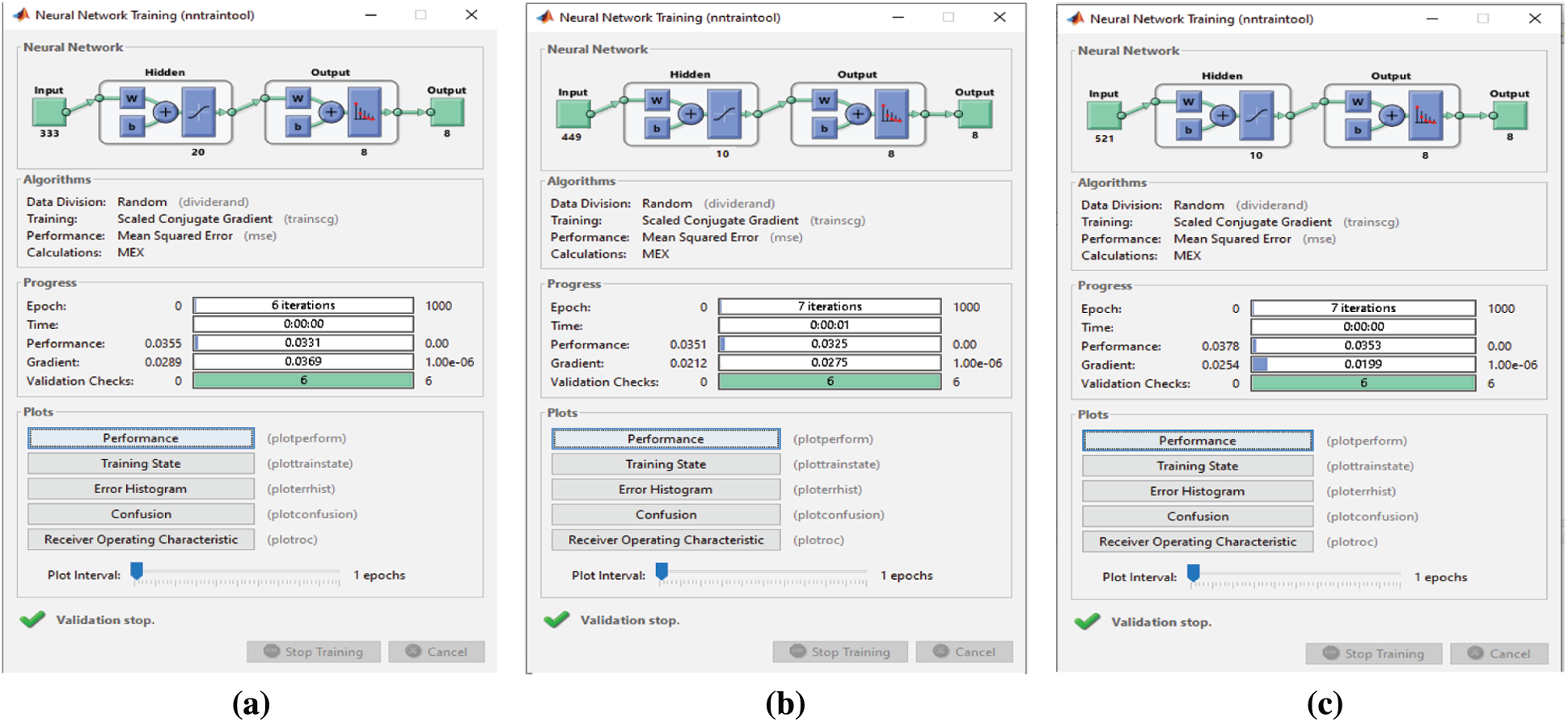
Figure 18: (a) NN training window after applying the proposed FS method on RAVDESS (b) NN training window after applying F-test on RAVDESS (c) NN training window after applying F-score on RAVDESS
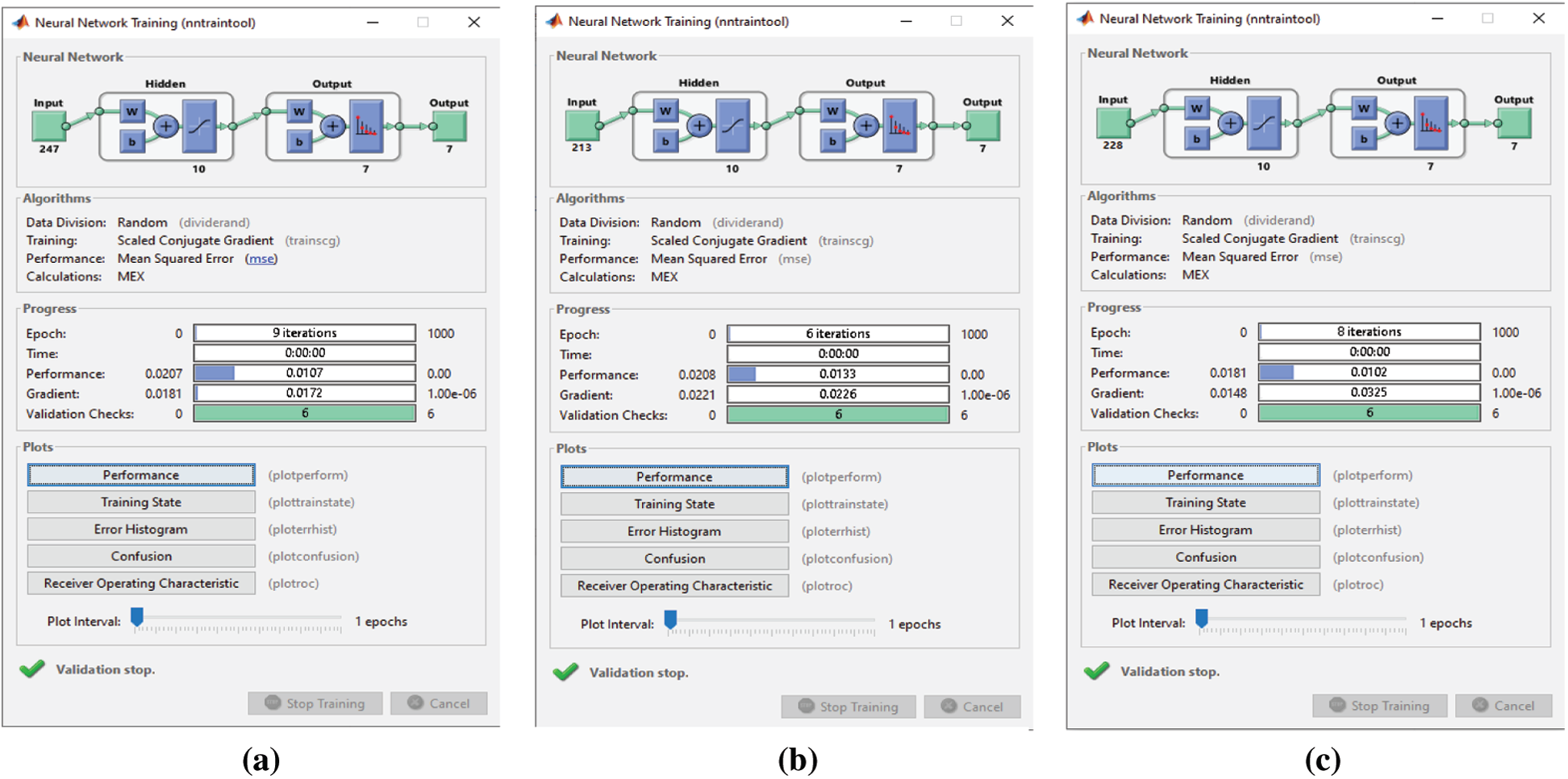
Figure 19: (a) NN training window after applying the proposed FS method on Emo-DB (b) NN training window after applying F-test on Emo-DB (c) NN training window after applying F-score on Emo-DB
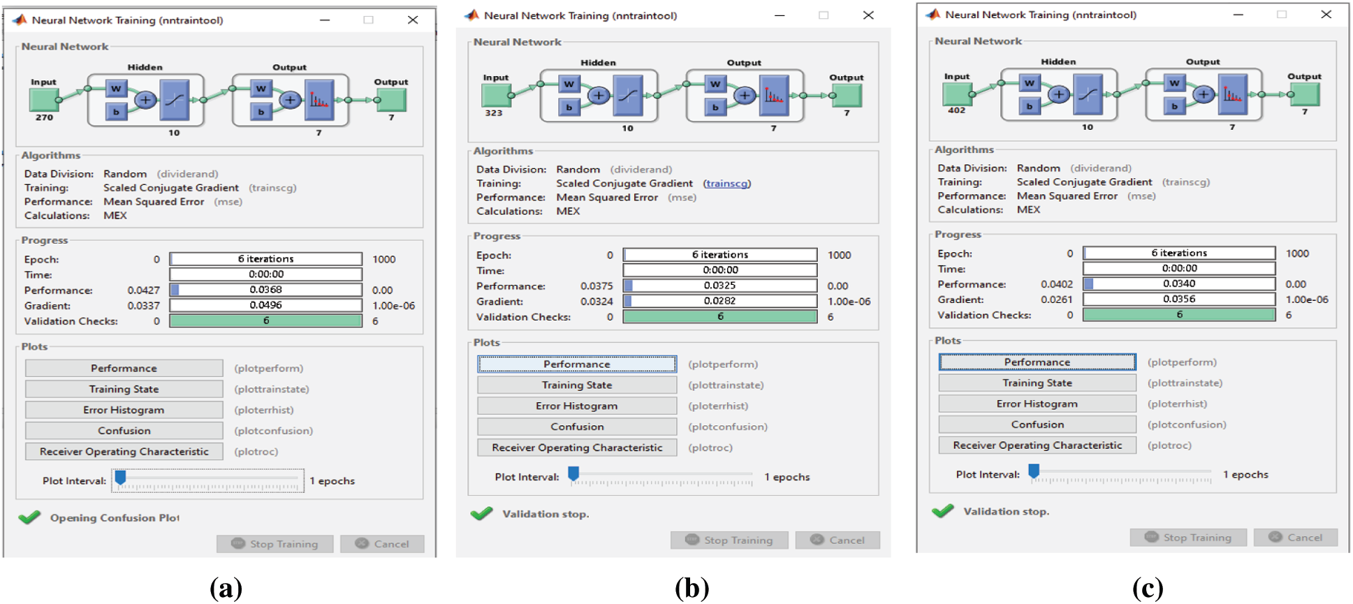
Figure 20: (a) NN training window after applying the proposed FS method on SAVEE (b) NN training window after applying F-test on SAVEE (c) NN training window after applying F-score on SAVEE
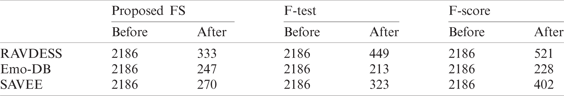
Before and after using the FS methods, six epochs are needed to classify the seven emotions in the SAVEE dataset (Figs. 17 and 20). Hence no improvement in classification time is achieved. Nevertheless, the classification accuracies are adequate, as discussed previously. Before applying the FS methods, 2,186 features are extracted from each audio file in the three datasets, because the same feature extraction process is applied to all three datasets. The number of features selected by the three FS methods are different (Tab. 5). Although the proposed FS method uses the fewest features from the RAVDESS dataset, it records the highest classification accuracy. The same is true for the SAVEE dataset. For the Emo-DB dataset, the proposed method achieves the highest accuracy in recognizing the seven emotions in the Emo-DB dataset and records the largest number of features.
Table 5: Numbers of features produced before and after implementing the FS methods
The confusion matrices in this study reveal a strong relationship between each FS method and the number of emotions. Each FS method affects the recognition of one or two emotions and affects different emotions. According to the results for the Emo-DB dataset, the proposed method negatively affects the accurate classification of happiness, the F-test FS method negatively affects the accurate classification of fear and anger, and the F-score FS method negatively affects the accurate classification of boredom. In summary, each FS method negatively affects the classification accuracy of a different emotion. Therefore, to build a hierarchical or ranking FS method from the three FS methods utilized in this work will result in Strong classification results, but it will consume more time. Ultimately, no relationship exists between the number of features, speed, and classification accuracy. The highest accuracy can be obtained with the lowest number of features, and the highest speed can be achieved with the largest number of features. The variation depends on the SoRV factor utilized in selecting the most powerful features in recognizing different emotions. Thus, to measure the power of classification for each feature is the key to the success of the proposed work. Specifically, many features can be excluded from the main feature domain because they are highly convergent but have high classification power. Such features are neglected by most FS methods. By contrast, our work assigns greater importance to the SoRV than to the QoPV because of its contribution to classification.
Acknowledgement: We thank LetPub (www.letpub.com) for its linguistic assistance during the preparation of this manuscript.
Funding Statement: The authors received no specific funding for this study.
Conflict of Interest: The authors declare that they have no conflicts of interest to report regarding the present study.
1. L. Yu and H. Liu, “Feature selection for high-dimensional data: A fast correlation-based filter solution,” in Proc. ICML, Washington, DC, USA, pp. 856–863, 2003. [Google Scholar]
2. P. Yang, B. B. Zhou, J. Y. yang and A. Y. Zomaya, “Stability of feature selection algorithms and ensemble feature selection methods,” in Bioinformatics, 1st ed., Hoboken, NJ, USA: John Wiley & Sons, Inc, pp. 333–352, 2013. [Google Scholar]
3. G. Chandrashekar and F. Sahin, “A survey on feature selection methods,” Computers and Electrical Engineering, vol. 40, no. 1, pp. 16–28, 2014. [Google Scholar]
4. G. James, D. Witten, T. Hastie and R. Tibshirani, An Introduction to Statistical Learning, 1sted., NY, USA: Springer, pp. 1–426, 2013. [Google Scholar]
5. B. Venkatesh and J. Anuradha, “A review of feature selection and its methods,” Cybernetics and Information Technologies, vol. 19, no. 1, pp. 3–26, 2019. [Google Scholar]
6. Y. Zhou, P. Utkarsh, C. Zhang, H. Ngo, X. Nguyen et al., “Parallel feature selection inspired by group testing,” in NIPS, Massachusetts, USA, pp. 3554–3562, 2014. [Google Scholar]
7. I. Guyon and A. J. J. o. m. l. r. Elisseeff, “An introduction to variable and feature selection,” Journal of Machine Learning Research, vol. 3, no. 3, pp. 1157–1182, 2003. [Google Scholar]
8. R. Panthong and A. Srivihok, “Wrapper feature subset selection for dimension reduction based on ensemble learning algorithm,” Procedia Computer Science, vol. 72, pp. 162–169, 2015. [Google Scholar]
9. A.-C. Haury, P. Gestraud and J.-P. Vert, “The influence of feature selection methods on accuracy, stability and interpretability of molecular signatures,” PLoS One, vol. 6, no. 12, pp. e28210, 2011. [Google Scholar]
10. I. Guyon, M. Nikravesh, S. Gunn and L. A. Zadeh, Embedded methods. In: Feature Extraction. Berlin, Germany: Springer, pp. 137–165, 2006. [Google Scholar]
11. D. Jain and V. Singh, “An efficient hybrid feature selection model for dimensionality reduction,” Procedia Computer Science, vol. 132, no. 2, pp. 333–341, 2018. [Google Scholar]
12. L. Yu and H. Liu, “Efficient feature selection via analysis of relevance and redundancy,” Machine Learning Research, vol. 5, no. 10, pp. 1205–1224, 2004. [Google Scholar]
13. S. Li, C. Liao and J. T. Kwok, “Gene feature extraction using T-test statistics and kernel partial least squares,” in Proc. ICONIP, Berlin Heidelberg: Springer-Verlag, pp. 11–20, 2006. [Google Scholar]
14. D. Liang, C. -F. Tsai and H. -T. Wua, “The effect of feature selection on financial distress prediction,” Knowledge-Based Systems, vol. 73, pp. 289–297, 2015. [Google Scholar]
15. E. E. Bron, M. Smits, W. J. Niessen and S. Klein, “Feature selection based on the SVM weight vector for classification of dementia,” Biomedical and Health Informatics, vol. 19, no. 5, pp. 1617–1626, 2015. [Google Scholar]
16. A. Bommert, X. Sun, B. Bischl, J. Rahnenführer and M. Lang, “Benchmark for filter methods for feature selection in high-dimensional classification data,” Computational Statistics and Data Analysis, vol. 143, no. 10, pp. 106839, 2020. [Google Scholar]
17. U. M. Khaire and R. Dhanalakshmi, “Stability of feature selection algorithm: A review,” Journal of King Saud University–Computer and Information Sciences, vol. 32, pp. 1–14, 2019. [Google Scholar]
18. N. Zhou and L. Wang, “A modified T-test feature selection method and its application on the HapMap genotype data,” Genomics, Proteomics & Bioinformatics, vol. 5, no. 3–4, pp. 242–249, 2007. [Google Scholar]
19. M. E. Ahsen, N. K. Singh, T. Boren, M. Vidyasagar and M. A. White, “A new feature selection algorithm for two-class classification problems and application to endometrial cancer,” in Proc. IEEE CDC, Maui, Hawaii, USA, pp. 2976–2982, 2012. [Google Scholar]
20. D. Wang, H. Zhang, R. Liu, W. Lv and D. Wang, “T-test feature selection approach based on term frequency for text categorization,” Pattern Recognition Letters, vol. 45, no. 1, pp. 1–10, 2014. [Google Scholar]
21. S. Sayed, M. Nassef, A. Badr and I. Farag, “A nested genetic algorithm for feature selection in high-dimensional cancer microarray datasets,” Expert Systems With Applications, vol. 121, no. 1, pp. 233–243, 2019. [Google Scholar]
22. Z. Yan, R. Khorasani, V. M. Levesque, V. H. Gerbaudo and P. B. Shyn, “Liver tumor F-18 FDG-PET before and immediately after microwave ablation enables imaging and quantification of tumor tissue contraction,” European Journal of Nuclear Medicine and Molecular Imaging, vol. 47, no. 12, pp. 1–8, 2020. [Google Scholar]
23. F. Zhang and F. Wang, “Exercise fatigue detection algorithm based on video image information extraction,” IEEE Access, vol. 8, pp. 199696–199709, 2020. [Google Scholar]
24. G. James, D. Witten, T. Hastie and R. Tibshirani, “Introduction to statistics,” in Statistical Methods for Astronomical Data Analysis, 8th ed., NY, USA: Springer, pp. 91–108, 2014. [Google Scholar]
25. P. J. H.o.c. Ekman and Emotion, “Basic emotions,” in Handbook of Cognition and Emotion, 8th ed., Chichester, West Sussex, UK: John Wiley & Sons, Inc., pp. 45–60, 1999. [Google Scholar]
26. T. Fawcett, “An introduction to ROC analysis,” Pattern Recognition Letters, vol. 27, no. 8, pp. 861–874, 2006. [Google Scholar]
 | This work is licensed under a Creative Commons Attribution 4.0 International License, which permits unrestricted use, distribution, and reproduction in any medium, provided the original work is properly cited. |