Computers, Materials & Continua DOI:10.32604/cmc.2021.012524
Article

Hydrodynamics and Sensitivity Analysis of a Williamson Fluid in Porous-Walled Wavy Channel

A. Shahzad1, W. A. Khan2,*, R. Gul1, B. Dayyan1 and M. Zubair1

1Department of Mathematics, COMSATS University Islamabad, Abbottabad Campus, 22060, Pakistan
2Department of Mechanical Engineering, College of Engineering Prince Mohammad Bin Fahd University, Al Khobar, 31952, Kingdom of Saudi Arabia
*Corresponding Author: W. A. Khan. Email: wkhan1956@gmail.com
Received: 10 August 2020; Accepted: 14 September 2020

Abstract: In this work, a steady, incompressible Williamson fluid model is investigated in a porous wavy channel. This situation arises in the reabsorption of useful substances from the glomerular filtrate in the kidney. After 80% reabsorption, urine is left, which behaves like a thinning fluid. The laws of conservation of mass and momentum are used to model the physical problem. The analytical solution of the problem in terms of stream function is obtained by a regular perturbation expansion method. The asymptotic integration method for small wave amplitudes and the RK-Fehlberg method for pressure distribution has been used inside the channel. It is demonstrated that the forward flow becomes fast in the narrow region (at x = 0.75), which dominates the upward flow inside the channel. To study the impact of model parameters on outputs, we applied normalized local sensitivity analysis and noticed that the most influential parameter for the longitudinal velocity profile is the dimensionless wave amplitude. The reabsorption parameter is sensitive for transverse velocity in the narrow region, and the Weissenberg number has a strong effect on the pressure inside the channel. Further, the least sensitive parameters for the velocity components and pressure have been identified.

Keywords: Sensitivity analysis; Williamson fluid; regular perturbation method; asymptotic approximation; RK-Fehlberg method; kidney flow

1  Introduction

Hydrodynamic in porous ducts (channel/tube) has been receiving the attention of many researchers in recent years because of its significant applications in several biological systems, particularly reabsorption of useful substances in the kidney. The kidney is an organ responsible for maintaining fluid, filtering minerals and regulating the blood pressure inside the several living bodies. The overall fluid inside the bodies is maintained in the functional unit of the kidney known as nephrons. Blood is filtered from glomerular collieries and enters the Bowman’s capsule called glomerular filtrate (GF). This filtrate contains substances, like water, about 95%, and other constituents like sodium (1.17g/L), potassium (0.750g/L), and chloride (1.87g/L) [1]. In normal (healthy) conditions, these substances are reabsorbed inside the body, and with the passage of time, GF reaches the end of the tubule behaving as a thin fluid called urine. The GF is considered the same as plasma of the blood without containing blood cells, but it comprises glucose, creatinine, proteins, urea, uric acid, and various ions. Water is assumed to be a Newtonian fluid in nature, obeying Newton’s law of viscosity [2]. While blood, saliva, glomerular filtrate, and excreta are biological fluids behaving as a non-Newtonian fluid [3].

In the literature, the flow of glomerular filtrate in the kidney has been discussed by several researchers. The pioneering work done by Macey [4] has been extended by several researchers assuming that GF behaves like a steady, creeping, incompressible and non-isothermal Newtonian fluid, while the geometry (shape) of the renal tubule is approximated with a straight or wavy channels/tubes [5–10]. In the last few years, Muthu et al. [11–14] studied the hydrodynamics of Newtonian fluid in a wavy channel. They obtained the series solution by assuming a large wavelength and discussed the importance of slope factor on fluid properties. Recently, his work has been extended by Javaria et al. [15], Farooq et al. [16] with assuming slip and magnetic field effects. In previous articles, there is a lack of information regarding the non-Newtonian nature of the GF, and only the Newtonian fluid model was taken into account.

The flow of GF inside the kidney is complex, and there are various non-Newtonian fluid models that are accepted as biological fluids. Williamson’s model is one in which the apparent viscosity varies gradually [17]. This model is characterized by shear thinning property, and several researchers have studied this model in peristalsis flow. Peristalsis flow of the Williamson model in the symmetric or asymmetric channel was studied by Nadeem et al. [18], and they reported that for small Williamson parameters, flow behaves like a Newtonian fluid. Later on, Akbar et al. [19] also studied the peristaltic flow of a Williamson fluid in an inclined asymmetric channel with partial slip. They found that with the rise in the Williamson parameter, the pressure decreases inside the channel. His work was extended by Nadeem et al. [20] with partial slip and heat transfer. They found that temperature decreases with increasing the Williamson parameter. Vajravelu et al. [21] studied the peristaltic flow of a Williamson fluid in asymmetric channels with leaky walls. They noted that the size of the trapped bolus decreases and its symmetry disappears for large values of the permeability parameter. Williamson fluid flow model is also analyzed by Akbar et al. [22,23] in stenosed arteries with porous walls. They also discussed the chemical reaction and heat transfer rate of Williamson fluid through a tapered artery with stenosis.

Within this work, a steady, incompressible Williamson fluid model in a porous wavy channel is investigated/developed, and normalized sensitivity analysis is performed. In a normalized local sensitivity analysis, the impact of a single model parameter is studied at a time on all output variables. Several researchers used this analysis in different biological engineering problems [24–28]. As mentioned in the previous paragraphs, that flow of GF inside the kidney is complex, and after the reabsorption of useful substances, its nature becomes thin to make the urine. Also, involved parameters in the model intended to simulate the uncertainty in the output. The main objective of this study is to investigate hydrodynamics and the impact of influential parameters on shear-thinning fluid (Williamson fluid) flow in a porous wavy channel having relevance with the flow of urine in the kidney. It is believed that this work is not published so far, and it will provide a good foundation and specialist knowledge in the field of analyzing the flow characteristics in the kidneys.

This paper is arranged as follows: Basic equations governing the flow of incompressible Williamson fluid inside the wavy porous walled channel are given in Section 2. Approximate solutions are obtained by using the Perturbation method in Section 3. Also, pressure distribution inside the channel is obtained by both asymptotic approximation of integration technique and numerically by the Runge-Kutta-Fehlberg method using MatLab. In Section 4, the effects of involved parameters are briefly discussed with the help of graphs and streamlines. A sensitivity analysis is performed in Section 5. Finally, the conclusion of the present study is presented in the last section.

2  Mathematical Formulation

Let us consider the flow of incompressible Williamson fluid in a porous walled wavy channel, with entrance flow rate Q0 and entrance pressure P0. The flow rate decays exponentially along the channel. The geometry of the problem is described in Fig. 1. The wall profile is defined as

h¯(x)=d+εsin(2πxλ),(1)

in which d is half-height of the channel at the entrance region, ε is the is amplitude and λ is the wavelength. It is noticed that for ε=d in one wavelength (λ=1) can show narrow (blockage) at x = 1/4.

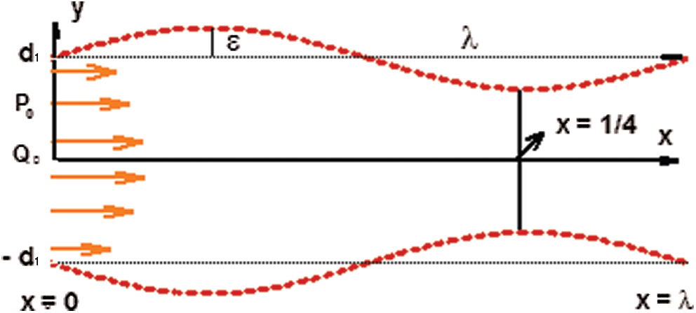
Figure 1: Geometry of the problem

The equations governing the flow of a Williamson fluid in the wavy channel are

divV=0, (2)

ρDVDt=divS+ρf (3)

where V is the velocity vector, ρ is the density, DDt represents the material derivative, S is the Cauchy stress tensor, f represents the body force and the extra stress tensor S for the Williamson fluid is defined as

S=-pI+τ¯, (4)

τ¯=[μ∞+(μ0+μ∞)(1-Γ|γ̇|)-1]γ̇, (5)

in which -pI is the spherical part of the stress due to constraint of incompressibility, τ¯ is the extra stress tensor, μ0 is the zero shear rate viscosity, μ∞ is the infinite shear rate viscosity, Γ is the time constant and |γ̇| is defined as

|γ̇|=12Π(6)

Here Π is the second invariant strain tensor. In Eq. (5), we consider the case for which μ∞=0 and Γ|γ̇|<1, therefore,

τ¯=[μ0(1+Γ|γ̇|)γ̇](7)

If Γ=0, the Newtonian fluid model can be recovered. For the two dimensional flow in the wavy channel, the Eqs. (1) and (2) in components form can be written as

∂u∂x+∂v∂y=0, (8)

ρ[u∂u∂x+v∂u∂y]=-∂p∂x+∂τ¯xx∂x+∂τ¯xy∂y, (9)

ρ[u∂v∂x+v∂v∂y]=-∂p∂y+∂τ¯yx∂x+∂τ¯yy∂y. (10)

where u and v are the velocity components, p is hydrodynamics pressure and τ¯xx, τ¯xy, τ¯yx, τ¯yy are the stress components. The boundary conditions of the problem are

u+dh¯(x)dxv=0aty=h¯(x), (11)

∂u∂y=0aty=0, (12)

Q(x)=2w∫0h¯(x)udy=Q0e-α¯x, (13)

p=P0atx=0. (14)

Eq. (11) shows the tangential velocity at the walls, while Eq. (13) shows the flow rate inside the channel, Q0 is the flow rate at x = 0, w is the width of the channel, and α¯ is reabsorption parameter [4]. To solve the model, Eqs. (8)–(14), let us introduce the non-dimensional variables defined by

x*=xλ,y*=yd,u*=dλuQ0,v*=λ2vQ0,δ=dλ,p*=d3pμQ0,ψ*=λψQ0(15)

and considering u*=∂ψ*∂x* and v*=-∂ψ*∂y*, Eqs. (9) and (10) in terms of stream function ψ* after dropping the asterisk sign (*) become

δRe[∂ψ∂y∂2ψ∂x∂y-∂ψ∂x∂2ψ∂y2]=-∂p∂x+δ2∂τxx∂x+∂τxy∂y (16)

-δ3Re[∂ψ∂y∂2ψ∂x2-∂ψ∂x∂2ψ∂x∂y]=-∂p∂y+δ2∂τyx∂x+δ∂τyy∂y. (17)

where the stress and strain tensors are defined by

τxx=2[1+Weγ̇]∂2ψ∂x∂y, (18)

τxy=[1+Weγ̇](∂2ψ∂y2-δ2∂2ψ∂x2), (19)

τyy=2δ[1+Weγ̇]∂2ψ∂x∂y. (20)

|γ̇|=[4δ2(∂2ψ∂x∂y)2+(∂2ψ∂y2-δ2∂2ψ∂x2)2]1/2. (21)

The boundary conditions are

∂ψ∂y-δ(1+εcos(2πx))∂ψ∂x=0ψ=γe-α¯xaty=η, (22)

∂2ψ∂y2=0ψ=0aty=0, (23)

p=P0atx=0,where,η=1+εsin(2πx). (24)

where Re=Q0νλ is Reynolds number, We=Q0Γλd2 is Weissenberg numbers, γ=λ2w is ratio of length to width, η=h(x)d is dimensionless wall profile, P0=μQ0P0d3 is dimensionless entrance pressure, and ε=kd is dimensionless amplitude, respectively. Using the assumptions of low Reynolds number and long wavelength and neglecting the terms of order δ and higher, Eqs. (15) and (16) take the form

0=-∂p∂x+∂∂y[1+We∂2ψ∂y2]∂2ψ∂y2, (25)

0=-∂p∂y. (26)

From Eq. (25), it is noticed that pressure depends on x only. Eliminating the pressure term from Eqs. (24) and (25), yield

0=∂2∂y2[1+We∂2ψ∂y2]∂2ψ∂y2,(27)

and the boundary conditions are

∂ψ∂y=0ψ=γe-αxaty=η, (28)

∂2ψ∂y2=0ψ=0aty=0, (29)

p=P0atx=0. (30)

where α=α¯λ is reabsorption parameter which controls the reabsorption across the walls. Eq. (26) along with boundary conditions (27)–(29) show the physical model showing the flow of Williamson fluid flow in the wavy channel. The solution of the developed model is solved by the perturbation method [29,30]. The solutions to the modeled problem are explained in the next section.

3  Solution of the Problem

Since Eq. (26) is a nonlinear partial differential equation, its exact solution is not possible; therefore, we chose the standard power series of the forms

ψ=ψ0+Weψ1+O(We)2…, (31)

p=p0+Wep1+O(We)2…, (32)

where the coefficient functions ψ0 and ψ1 are independent of We. Substituting the above expressions in Eqs. (24) and (26) and boundary conditions (27) to (29), we get.

3.1 System of Order We0

The coefficients of zeroth order are equated on both sides of Eq. (26) to get

∂4ψ0∂y4=0, (33)

dp0dx=∂3ψ0∂y3, (34)

and the boundary conditions

∂ψ0∂y=0ψ0=γe-αxaty=η, (35)

∂2ψ0∂y2=0ψ0=0aty=0. (36)

The solution of Eqs. (31)–(33) is obtained as

ψ0=-12Q(x)y(-3η2+y2)η3.(37)

Using Eq. (36) in Eq. (33), we find

dp0dx=-3γe-αxη3=-3Q(x)η3.(38)

Eqs. (36) and (37) contains the effects of flow rate Q(x)=γe-αx.

3.2 System of Order We1

The first-order problem is obtained by equating the power of We1, we get

∂4ψ∂y4+∂2∂y2(∂2ψ0∂y2)2=0, (39)

dp1dx=∂3ψ1∂y3+2(∂2ψ0∂y2)2∂3ψ0∂y3., (40)

with boundary conditions

∂ψ1∂y=0ψ1=0aty=η, (41)

∂2ψ1∂y2=0ψ1=0aty=0. (42)

The solution of the Eq. (35) with boundary conditions (36), (37) is

ψ1=-38(Q(x))2y(η3-3y2η+2y3)η6.(43)

using Eqs. (36) and (42) in Eq. (39), we get

dp1dx=27(Q(x))24η5.(44)

Using Eqs. (36) and (42) in Eq. (30), the expression for stream function becomes

ψ=-12Q(x)(-3η2+y2)yη3-3We8(Q(x))2(η3-3y2η+2y3)yη6+…(45)

The zeroth-order solution of Muthu et al. [11] can be retrieved when We→0. Using Eqs. (37) and (43) in Eq. (31), we get the pressure gradient in the following form

dpdx=-3Q(x)η3+27We(Q(x))24η5+…(46)

To get the expression for pressure with boundary condition,

p=P0atx=0,(47)

an exact solution for pressure cannot be obtained. Approximate solutions of Eq. (45) with boundary condition (46) are obtained by asymptotic approximation of integration technique for ε→0, [29,30], and numerically by Runge-Kutta-Fehlberg method using MATLAB software.

The expression for pressure in term of elementary functions, using an asymptotic approximation of integration technique for ε→0 is

p(x)=135Weγ2ε(cos(2πx)π+αsin(2πx))e-2αx8α2+8π2-3γe-αx(3α2εsin(2πx)+6παεcos(2πx)-α2-4π2)(α2+4π2)α-27γ2(e-αx)2We8α+C1,(48)

where,

C1=P0-135γ2Weεπ8α2+8π2+27γ2We8α+18γεπα2+4π2-3γα.(49)

which depends upon ε, We and α.

4  Result and Discussion

Graphical behavior of velocity components, pressure distribution, and stream function are observed for different Weissenberg numbers We, reabsorption parameter α, and wave amplitude ε. In this study x = 0, and x = 1 indicate the entrance, and exit regions of the rectangular cross-section of the wavy channel, respectively.

In Figs. 2 and 3, the effects of We on both the components of velocity, i.e., longitudinal and transverse are studied at the entrance x = 0 and exit x = 1 of the channel. Fig. 2a indicates that at the centerline, longitudinal velocity decreases by increasing the magnitude of We, while due to the wall friction, the opposite nature of fluid flow is noticed near the walls. Similarly, transverse velocity increases by increasing We near the wall while near the centerline, it decreases due to the rise in pressure drop, see Fig. 2b.

At the exit region, both components of velocity have the same nature as that of the entrance region, see Figs. 2 and 5. It is observed that the dimensionless velocity at the entrance (x=0) is higher as compared to the exit region of the channel.

Figs. 4 and 5 illustrate the variations of the reabsorption parameter α on components of velocity at the entrance and exit regions of the channel. Fig. 4a depicts that no effect of α is observed on the longitudinal velocity at the entrance region, while transverse velocity shows significant effects. Transverse velocity first increases from the centerline; then, it shows a downfall towards the walls of the channel. Also, increasing α its profile increases due to the seepage of the fluid across the wall of the channel and then decreases at the channel wall, Fig. 4b.

The variation of α on longitudinal and transverse velocities inside the channel at the exit regions is displayed in Figs. 5a and 5b. It is noticed that near the center of the channel, flow is maximum due to the pressure gradient, and near the walls, the fluid flow becomes stationary due to wall friction and fluid viscosity. With increasing α longitudinal velocity decreases, while opposite behavior transverse velocity is controlled by α, see Fig. 5b. For higher α, transverse velocity upturns with no reversal of fluid. At the exit region, longitudinal velocity shows low profile behavior due to an increase in α. While transverse velocity near the wall shows a higher velocity profile.

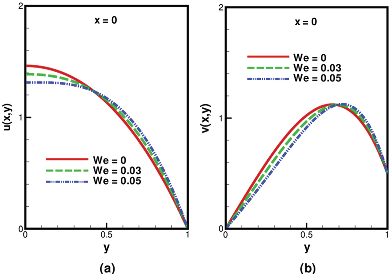
Figure 2: Variation of We on (a) longitudinal velocity (b) transverse velocity inside the channel at the entrance, when γ=1, α=0.5 and ε=0.2

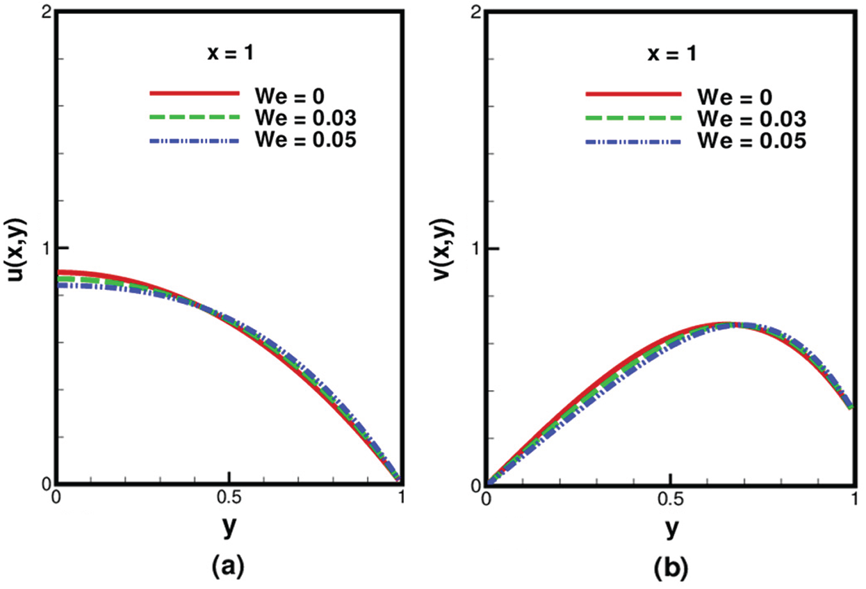
Figure 3: Variation of We on (a) longitudinal velocity (b) transverse velocity inside the channel at the exit, when γ=1, α=0.5 and ε=0.2

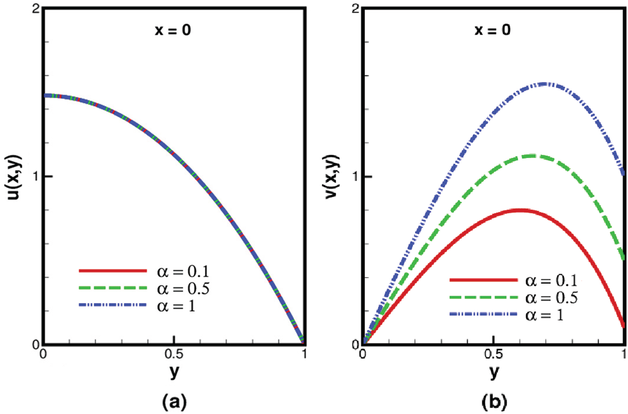
Figure 4: Variation of α on (a) longitudinal velocity (b) transverse velocity inside the channel at the entrance, when γ=1, We = 0.05 and ε=0.2

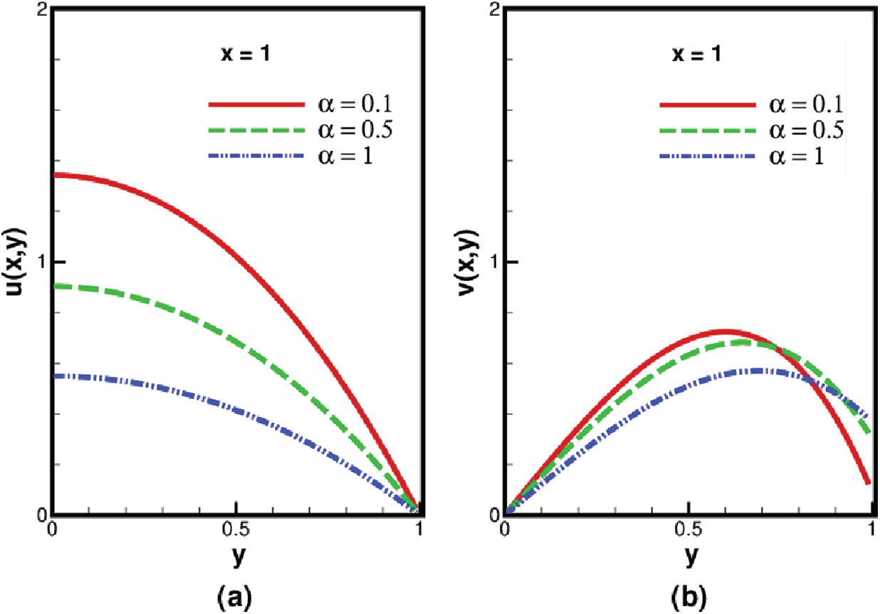
Figure 5: Variation of α on (a) longitudinal velocity (b) transverse velocity inside the channel at the exit region, when γ=1, We = 0.05 and ε=0.2

The variation of ε on longitudinal and transverse velocities inside the channel at the entrance and exit regions is presented in Figs. 6 and 7. It is important to note that no appreciable effect of ε on the longitudinal velocity at the entrance and exit regions of the channel, see Figs. 6a and 7a. However, due to higher values of ε, transverse velocity indicates reverse flow due to the narrowing of the walls 2. At the exit of the channel, the same behavior of fluid flow is noticed as that in the entrance region, see Figs. 6b and 7b. The velocity profile at the entrance (x=0) is observed higher as compared to the exit region due to the fluid seepage across the walls of the channel.

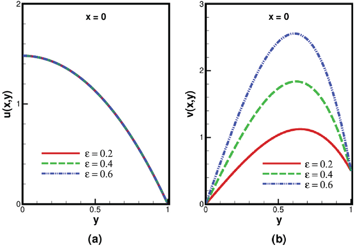
Figure 6: Variation of ε on (a) longitudinal velocity (b) transverse velocity inside the channel at the entrance region, when γ=1, We = 0.05 and α=0.5

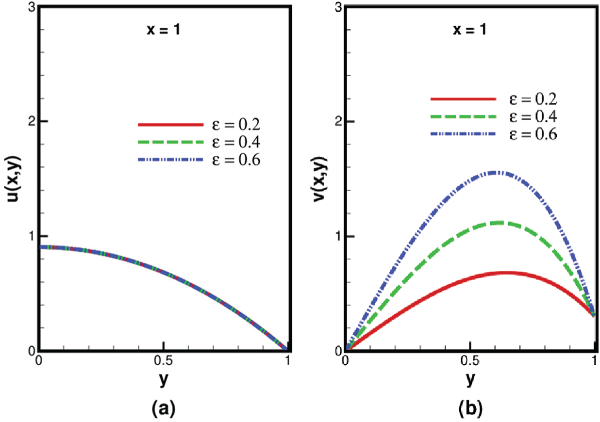
Figure 7: Variation of (a) longitudinal velocity, and (b) transverse velocity with ε inside the channel at the exit region, when γ=1, We = 0.05 and α=0.5

Figs. 8a–8c illustrate the variation of We, α and ε on the pressure inside the channel. It is observed that pressure decreases from the entrance to the exit of the channel. With increasing We, α and ε pressure increases due to the leakage of the fluid across the channel walls. Further, the asymptotic solution of the complicated integral validates the numeric results.

Finally, Figs. 9–11 are plotted to examine the influence of the pertinent parameters such as We, α and ε on the streamline pattern inside the wavy channel. The streamlines represent a path followed by a fluid particle during its motion. In Fig. 9, with increasing We, maximum fluid for fixed values of α and ε goes outside from the exit region of the channel. While for the fixed values of We and ε, fluid leakage increases with increasing α across the walls, see Fig. 10. The geometry is controlled by ε, see Fig. 11 and with increasing ε fluid before entering a narrow region shows significant changes.

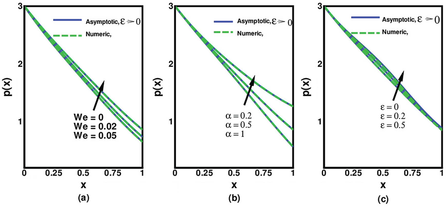
Figure 8: Variation of pressure inside the channel with (a) We when α=0.5, ε=0.2, (b) α when We = 0.05, ε=0.2 and (c) ε when α=0.5, We = 0.05 for γ=1

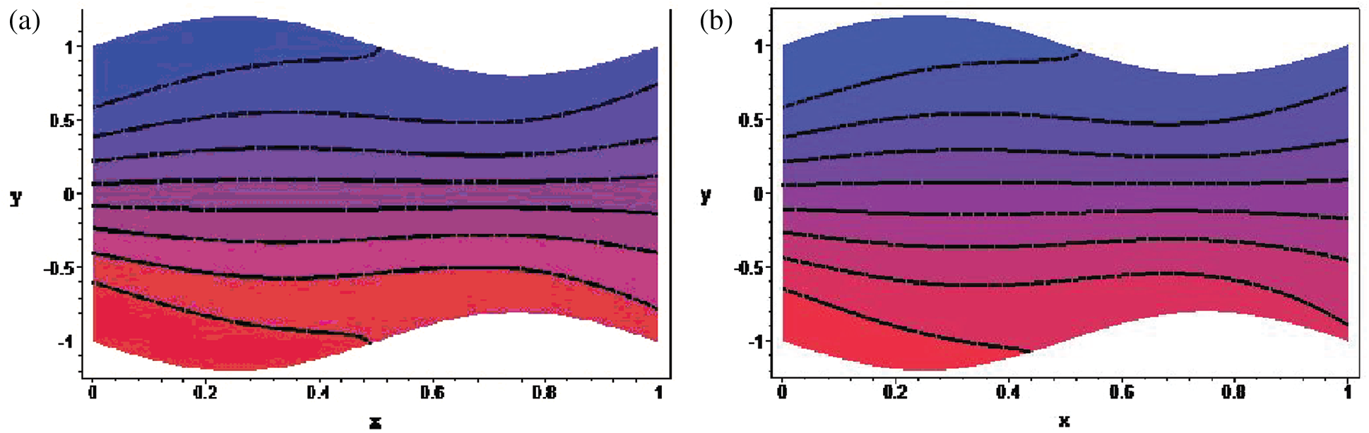
Figure 9: Streamline pattern inside the channel for (a) We = 0.01 and (b) We = 0.05 with fixed α=0.5, γ=1 and ε=0.2

The foregoing discussion reveals that the parameters We, α, δ and ε affect the velocity components and pressure inside the channel. As mentioned earlier, that sensitivity analysis is necessary to examine the impact of input parameters We, α, δ and ε on outputs like velocity components (u,v) and pressure p. This analysis will be helpful for the researcher during the experimental validation of GF in the kidney.

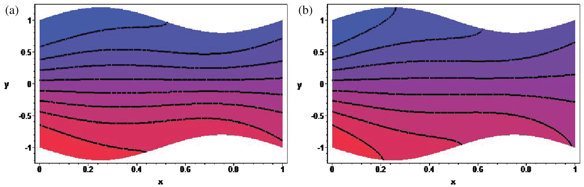
Figure 10: Streamline pattern inside the channel for (a) α=0.5 and (b) α=1 with fixed ε=0.2, γ=1 and We = 0.05

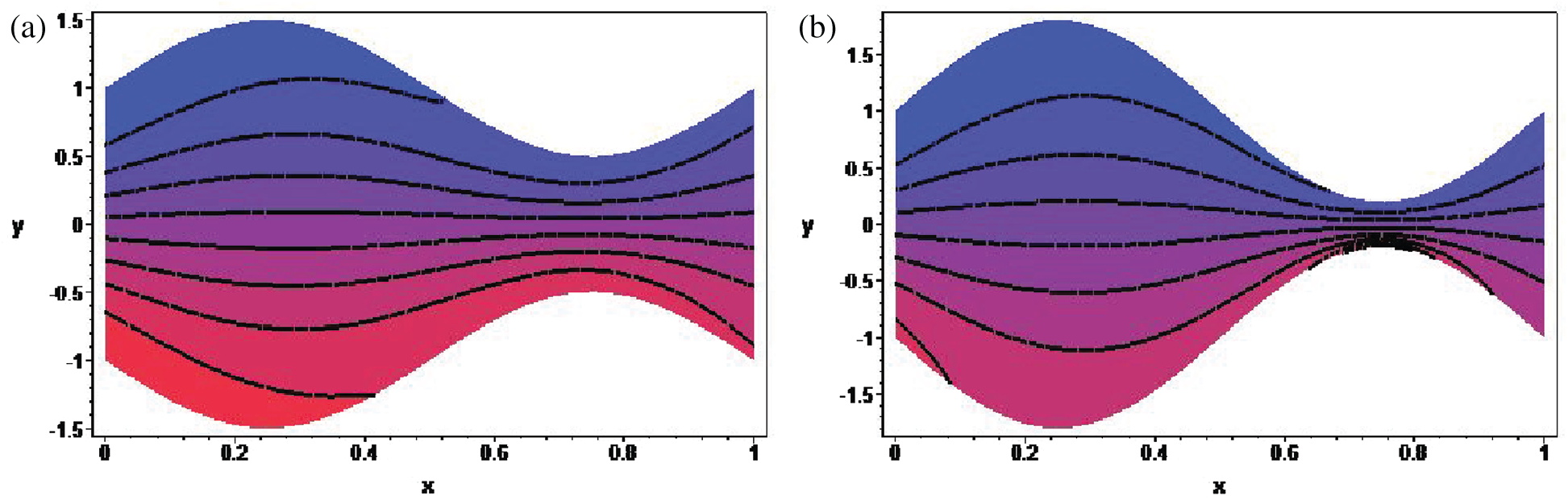
Figure 11: Streamline pattern inside the channel for (a) ε=0.5 and (b) ε=0.8 with fixed α=0.5, γ=1 and We = 0.05

5  Sensitivity Analysis (SA)

Sensitivity analysis is the method in which we study the impact of model parameters (input quantities of interest, QoI) on output variables (output quantities of interest, QoI). In this study, the input QoI are We, α, ε and δ, while output QoI are the velocity components (u,v) and pressure p. All input parameters are perturbed 0.2%, 1% and 2% from their nominal values one by one, and their impacts are quantified on output QoI. For the sake of simplicity, here we only presented the impact of 2% change of each input QoI on output QoI using the following relationship:

Sij=∂θ∂X≅θ(X+ΔX)-θ(X)ΔX,N=1n∑ Sij

Table 1: Sensitivity analysis of crucial parameters in the narrow region of the channel

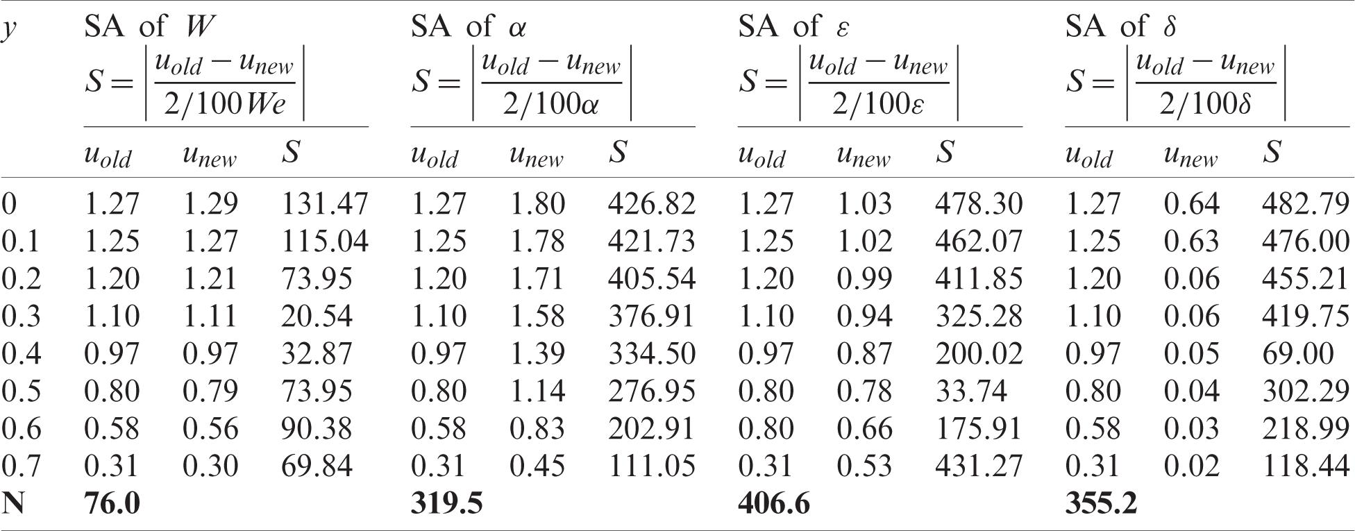
where Sij is the sensitivity indices for ith model outputs with respect to jth input parameters, n is the mesh size and N is the magnitude of sensitivity. Tab. 1 shows the results of the sensitivity of longitudinal velocity for the fixed values of α, δ and ε, while a 2% change in We, α, ε and δ is considered. It is noticed that ε is the most influential parameter for the longitudinal velocity at the narrow region of the channel, while, We is the least critical parameter in this region. For comparison, Fig. 12a shows that δ is even more important than We and α. Also, the major impact of ε is found on the channel wall. In Fig. 12b, it is observed that α is the most influential parameter for the transverse components of velocity in the narrow region and We has no effects in this region. Again the significant impact of α is noticed at the wall of the channel. The effects of input parameters on the pressure inside the channel is also analyzed and displayed in Fig. 12c. It is observed that We becomes the most crucial parameter as compared to α, ε and δ.

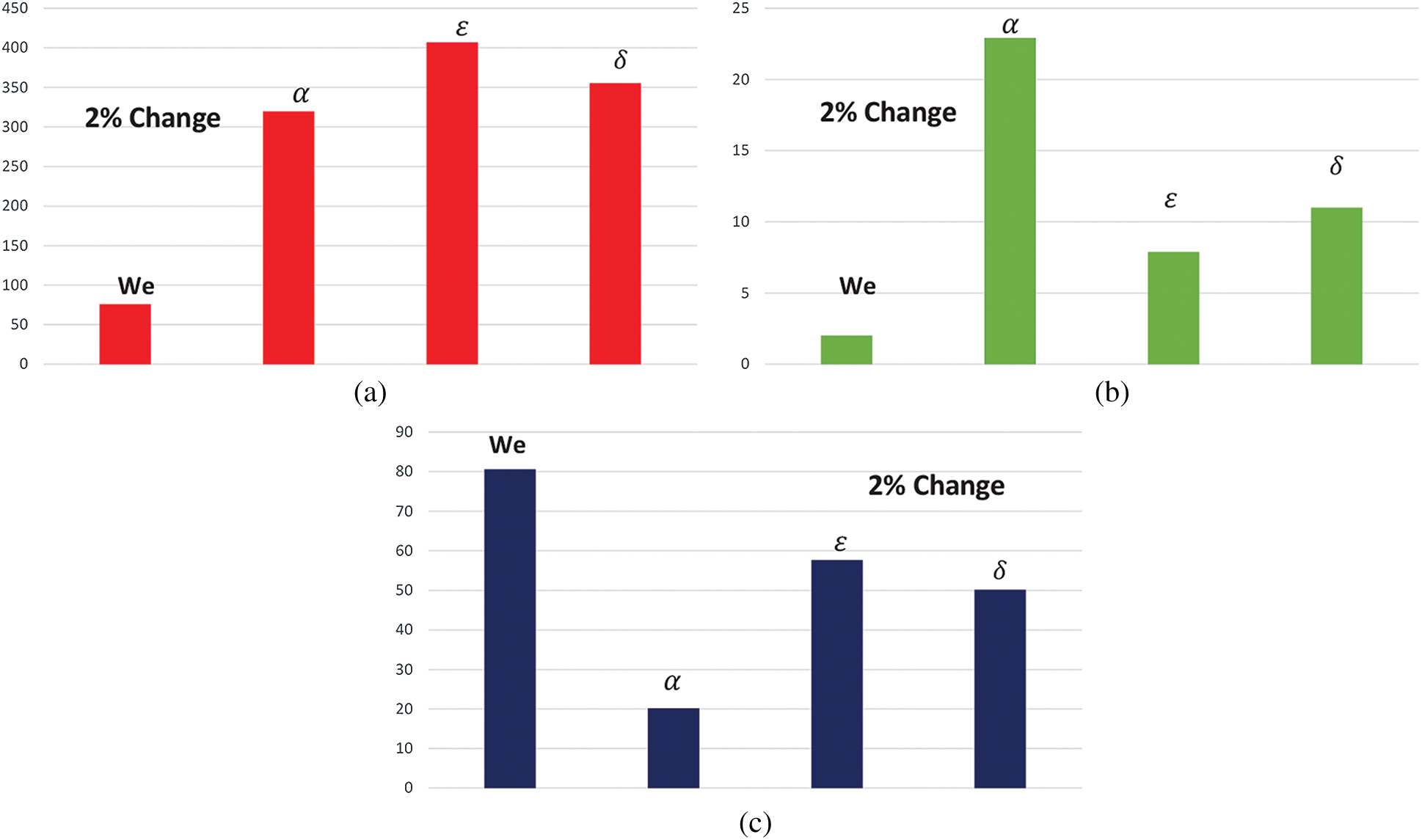
Figure 12: Sensitivity analysis results of (a) longitudinal velocity, (b) transverse velocity in the narrow region, and (c) pressure inside the channel

6  Conclusions

A mathematical model has been developed for the flow and sensitivity analysis of Williamson fluid in a porous wavy channel. The nonlinear PDEs are reduced by using the stream function and are solved by a regular perturbation method. An asymptotic integral method for small wave amplitude has been used to get the pressure in terms of elementary function. In contrast, the RK-Fehlberg method is used to get the numerical solution for the pressure in the channel. The sensitivity analysis is used to quantify the effects of input parameters on model outputs, such as velocity components and pressure inside the channel. The essential conclusions of this study are summarized below:

1.    The flow becomes fast in the narrow region, which dominates the upward flow.

2.    The pressure decays along the channel.

3.    The velocity profile is higher at the entrance as compared to the exit region of the channel.

4.    For longitudinal velocity in the narrow region, the dimensionless amplitude is the most influential parameter, and the Weissenberg number is the least essential parameter.

5.    The reabsorption parameter is sensitive to the transverse velocity at the narrow region of the channel.

6.    In case of pressure, the Weissenberg number is the most influential parameter, while the reabsorption parameter shows less sensitivity.

7.    The significant impact of velocity components is found at the wall of the channel.

Funding Statement: The author(s) received no specific funding for this study.

Conflicts of Interest: The authors declare that they have no conflicts of interest to report regarding the present study.

References

 1.  E. H. Starling, “The glomerular functions of the kidney,” Journal of Physiology, vol. 24, no. 3–4, pp. 317–330, 1899. [Google Scholar]

 2.  D. M. William, B. Satvat and J. M. Jamieson, “Theoretical model for glomerular filtration of charged solutes,” American Journal of Physiology-Renal Physiology, vol. 238, no. 2, pp. F126–F139, 1980. [Google Scholar]

 3.  P. Chaturani and R. Ponnalagar Samy, “A study of non-Newtonian aspects of blood flow through stenosed arteries and its applications in arterial diseases,” Biorheology, vol. 22, no. 6, pp. 521–531, 1985. [Google Scholar]

 4.  I. R. Macey, “Pressure flow patterns in a cylinder with reabsorbing walls,” Bulletin of Mathematical Biophysics, vol. 25, no. 1, pp. 1–9, 1963. [Google Scholar]

 5.  A. A. Kozinski, F. P. Schmidt and E. N. Lightfoot, “Velocity profiles in porous-walled ducts,” Industrial and Engineering Chemistry Fundamentals, vol. 9, no. 3, pp. 502–505, 1970. [Google Scholar]

 6.  R. Macey, “Hydrodynamics in the renal tubule,” Bulletin of Mathematical Biophysics, vol. 27, no. 2, pp. 117–124, 1965. [Google Scholar]

 7.  E. A. Marshall and E. A. Trowbridge, “Flow of a Newtonian fluid through a permeable tube: The application to the proximal renal tubule,” Bulletin of Mathematical Biology, vol. 36, no. 5–6, pp. 457–476, 1974. [Google Scholar]

 8.  G. Radhakrishnamacharya, P. Chandra and M. R. Kaimal, “A hydrodynamical study of the flow in renal tubules,” Bulletin of Mathematical Biology, vol. 43, no. 2, pp. 151–163, 1981. [Google Scholar]

 9.  E. A. Marshall and E. A. Trowbridge, “A mathematical model of the ultra-filtration process in a single glomerular capillary,” Journal of Theoretical Biology, vol. 48, no. 2, pp. 389–412, 1974. [Google Scholar]

10. A. M. Siddiqui, T. Haroon and A. Shahzad, “Hydrodynamics of viscous fluid through porous slit with linear absorption,” Applied Mathematics and Mechanics, vol. 37, no. 3, pp. 361–378, 2016. [Google Scholar]

11. P. Muthu and T. Berhane, “Flow through nonuniform channel with permeable wall and slip effect,” Special Topics and Reviews in Porous Media: An International Journal, vol. 3, no. 4, pp. 321–328, 2012. [Google Scholar]

12. P. Muthu and T. Berhane, “Fluid flow in a rigid wavy nonuniform tube: Application to flow in renal tubules,” APRN Journal of Engineering and Applied Sciences, vol. 5, no. 1, pp. 15–21, 2010. [Google Scholar]

13. P. Muthu and T. Berhane, “Fluid flow in asymmetric channel,” Tamkang Journal of Mathematics, vol. 42, no. 2, pp. 149–162, 2011. [Google Scholar]

14. P. Muthu and M. Varunkumar, “Mathematical model of flow in a doubly constricted permeable channel with effect of slip velocity,” Journal of Applied Nonlinear Dynamics, vol. 8, no. 4, pp. 655–666, 2019. [Google Scholar]

15. J. F. Javaria, J. D. Chung, M. Mushtaq, D. Lu, M. Ramazan et al., “Influence of slip velocity on the flow of viscous fluid through a porous medium in a permeable tube with a variable bulk flow rate,” Results in Physics, vol. 11, no. 12, pp. 861–868, 2018. [Google Scholar]

16. J. Farooq, M. Mushtaq, S. Munir, M. Ramzan, J. D. Chung et al., “Slip flow through a nonuniform channel under the influence of transverse magnetic field,” Scientific Reports, vol. 8, no. 1, pp. 131–137, 2018. [Google Scholar]

17. S. Nadeem and S. Akram, “Peristaltic flow of a Williamson fluid in an asymmetric channel,” Communications in Nonlinear Science and Numerical Simulation, vol. 15, no. 7, pp. 1705–1716, 2010. [Google Scholar]

18. S. Nadeem and S. Akram, “Influence of inclined magnetic field on peristaltic flow of a Williamson fluid model in an inclined symmetric or asymmetric channel,” Mathematical and Computer Modelling, vol. 52, no. 1–2, pp. 107–119, 2010. [Google Scholar]

19. N. S. Akbar, T. Hayat, S. Nadeem and S. Obaidat, “Peristaltic flow of a Williamson fluid in an inclined asymmetric channel with partial slip and heat transfer,” International Journal of Heat and Mass Transfer, vol. 55, no. 7–8, pp. 1855–1862, 2012. [Google Scholar]

20. S. Nadeem and S. Akram, “Influence of inclined magnetic field on peristaltic flow of a Williamson fluid model in an inclined symmetric or asymmetric channel,” Mathematical and Computer Modelling, vol. 52, no. 1–2, pp. 107–119, 2010. [Google Scholar]

21. K. Vajravelu, S. Sreenadh, K. Rajanikanth and C. Lee, “Peristaltic transport of a Williamson fluid in asymmetric channels with permeable walls,” Nonlinear Analysis: Real World Applications, vol. 13, no. 6, pp. 2804–2822, 2012. [Google Scholar]

22. N. S. Akbar, S. Nadeem and C. Lee, “Influence of heat transfer and chemical reactions on Williamson fluid model for blood flow through a tapered artery with a stenosis,” Asian Journal of Chemistry, vol. 24, no. 6, pp. 2433–2441, 2012. [Google Scholar]

23. N. S. Akbar, S. U. Rahman, R. Ellahi and S. Nadeem, “Blood flow study of Williamson fluid through stenosed arteries with permeable walls,” European Physical Journal Plus, vol. 129, no. 11, pp. 1–10, 2014. [Google Scholar]

24. R. Gul and S. Shahzadi, “Beat-to-beat sensitivity analysis of human systemic circulation coupled with the left ventricle model of the heart: A simulation-based study,” European Physical Journal Plus, vol. 134, no. 7, pp. 1–23, 2017. [Google Scholar]

25. R. Gul, A. Shahzad and M. Zubair, “Application of 0D model of blood flow to study vessel abnormalities in the human systemic circulation: An in-silico study,” International Journal of Biomathematics, vol. 11, no. 8, pp. 1850106, 2018. [Google Scholar]

26. R. Gul, N. Shaheen and A. Shahzad, “Personalized mathematical model of human arm arteries with inflow boundary condition,” European Physical Journal Plus, vol. 135, no. 1, pp. 1–14, 2020. [Google Scholar]

27. H. Yuan, B. Suki and K. R. Lutchen, “Sensitivity analysis for evaluating nonlinear models of lung mechanics,” Annals of Biomedical Engineering, vol. 26, no. 2, pp. 230–241, 1998. [Google Scholar]

28. C. Thamrin, Z. T. Cindy, J. A. Rachel, A. Collins, P. D. Sly et al., “Sensitivity analysis of respiratory parameter estimates in the constant-phase model,” Annals of Biomedical Engineering, vol. 32, no. 6, pp. 815–822, 2004. [Google Scholar]

29. A. W. Bush, Perturbation Methods for Engineers and Scientists. England, UK: Routledge, 2018. [Google Scholar]

30. V. D. Milton, Perturbation Methods in Fluid Mechanics. New York: Parabolic Press, 1975. [Google Scholar]

This work is licensed under a Creative Commons Attribution 4.0 International License, which permits unrestricted use, distribution, and reproduction in any medium, provided the original work is properly cited.