Computers, Materials & Continua DOI:10.32604/cmc.2021.012252
Article

Segmentation of Brain Tumor Magnetic Resonance Images Using a Teaching-Learning Optimization Algorithm

J. Jayanthi1,*, M. Kavitha2, T. Jayasankar3, A. Sagai Francis Britto4, N. B. Prakash5, Mohamed Yacin Sikkandar6 and C. Bharathiraja7

1Department of Computer Science and Engineering, Sona College of Technology, Salem, 636005, Tamilnadu, India
2Department of Electronics and Communication Engineering, K. Ramakrishnan College of Technology, Trichy, 621112, India
3Department of Electronics and Communication Engineering, University College of Engineering, Anna University, Tiruchirappalli, 620024, India
4Department of Mechanical Engineering, Rohini College of Engineering and Technology, Palkulam, 629401, India
5Department of Electrical and Electronics Engineering, National Engineering College, Kovilpatti, 628503, India
6Department of Medical Equipment Technology, College of Applied Medical Sciences, Majmaah University, AlMajmaah, 11952, Kingdom of Saudi Arabia
7Department of Electrical and Electronics Engineering, SRM Institute of Science and Technology, Chennai, 603203, India
*Corresponding Author: J. Jayanthi. Email: jayanthisnt@yahoo.com
Received: 30 August 2020; Accepted: 13 March 2021

Abstract: Image recognition is considered to be the pre-eminent paradigm for the automatic detection of tumor diseases in this era. Among various cancers identified so far, glioma, a type of brain tumor, is one of the deadliest cancers, and it remains challenging to the medicinal world. The only consoling factor is that the survival rate of the patient is increased by remarkable percentage with the early diagnosis of the disease. Early diagnosis is attempted to be accomplished with the changes observed in the images of suspected parts of the brain captured in specific interval of time. From the captured image, the affected part of the brain is analyzed using magnetic resonance imaging (MRI) technique. Existence of different modalities in the captured MRI image demands the best automated model for the easy identification of malignant cells. Number of image processing techniques are available for processing the images to identify the affected area. This study concentrates and proposes to improve early diagnosis of glioma using a preprocessing boosted teaching and learning optimization (P-BTLBO) algorithm that automatically segments a brain tumor in an given MRI image. Preprocessing involves contrast enhancement and skull stripping procedures through contrast limited adaptive histogram equalization technique. The traditional TLBO algorithm that works with the perspective of teacher and the student is here improved by using a boosting mechanism. The results obtained using this P-BTLBO algorithm is compared on different benchmark images for the validation of its standard. The experimental findings show that P-BTLBO algorithm approach outperforms other existing algorithms of its kind.

Keywords: Brain tumor; TLBO algorithm; skull stripping; preprocessing; segmentation

1  Introduction

Brain tumors are considered one of the most life-threatening conditions. A tumor in one area of the brain is normally activated and spreads to adjacent areas [1]. The high morbidity and mortality rates of a glioma, a type of brain tumor, have been described in the literature. A tumor is considered a low-or high-grade glioma [2] based on its severity. New medical methods are used for initial diagnosis and validation screening. To identify the site and condition of a glioma can lead to effective treatment, which may include radiation therapy, chemotherapy, and surgery. Tumor development is limited by radiation and chemotherapy, and surgery is used to eliminate the whole affected section. Magnetic resonance imaging (MRI) is the best imaging tool for the detection of brain abnormalities as assessed in clinical trials. Advanced MRI equipment provides complete three-dimensional (3D) views of the internal parts of the brain. 3D or cut MRI images are captured, and the location of the disease is determined on this basis. Image processing allows the assessment of the severity of the problem, and appropriate care can be sought.

Various techniques used to identify abnormalities present in MRI images have been described in surveys of existing methods. They include neural network (NN)-based methods [3], watershed segmentation [4], clustering techniques, fuzzy c-means (FCM), edge detection, the adaptive neuro-fuzzy inference system (ANFIS), the Gaussian mixture method, cellular automation, multi-level thresholding, and heuristic techniques. A study showed that the hybridization of a few methods could have the highest possible segmentation accuracy [5]. Brain tumor segmentation approaches, in addition to methods focused on neural networks [6], collect MRI images based on particular modalities. This approach is used to accurately segment and diagnose MRI datasets that have classified modalities, such as fluid-attenuated inversion recovery (FLAIR), spin-lattice relaxation (T1), enhanced T1-contrast (T1C), and spin relaxation (T2). This study proposes a technique to identify the tumor region and edema area in an MRI image using the FLAIR, T1C, and T2 methods, based on metaheuristic optimization.

Numerous experiments have been conducted in medical image processing, including fundamental work on MRI imaging strategies such as grouping strategies, clustering techniques, and meta-heuristic techniques. A number of image segmentation techniques are used to process medical diagnostic images. Earlier studies [7] proposed FCM and k-means clustering, a flexible and simple technique to identify tumors. The k-means technique minimizes the time needed for analysis, but is not best suited for chronic tumor diseases, while FCM requires a noise-free image. KIFCM combines k-means and FCM to resolve the limitation of high iterations and improve the precision of classification, and is recommended for optimum results. A procedure that uses color transformation and k-means converts a grey image to a color image to define the exact malignant region, increasing the accuracy of the assessment of the precise size of a tumor [8].

Extraction methods commonly used to classify the brain tumor area in an MRI image have been tested [9]. The brain is highly complex, and it is challenging to highlight specific regions of it in MRI images. Hence the best image processing technique is needed. One such method employs multi functional Brownian motion and uses spatially complex multi-fractal highlights for classification. This model uses AdaBoost, which minimizes the exponential loss function, and this method helps to distribute the weight of the classifier to maximize its output. One such technique is used to preserve high-level information derived from the original image [10]. The heterogeneous design of the PC-dependent classification technique is used to distinguish the edges between malignant cells in MRI images. FCM uses spatial data to segment MRI images. FCM and k-means were used in a method to remove tumor cells from a complicated MRI image by a histogram-directed installation technique [11]. A deep learning algorithm was used to simplify the process of brain tumor segmentation [12]. A thorough overview of the methods used to strip noise from tumor-affected brain images, including wavelet, curvelet, and filter templates, was published [13].

A tool was developed to classify the types of histopathological photographs of brain tumors that should be predicted early [14]. A vision technique using reverberation spectroscopy was employed to mechanically isolate brain tumors [15]. An automatic detection model was used to segregate MRI brain images to determine tumor locations [16]. This study proposes an automatic preprocessing boosted teaching and learning optimization (P-BTLBO) algorithm for brain tumor MRI image sections. Contrast enhancement and skull stripping procedures are accomplished through preprocessing. Conventional TLBO algorithms are strengthened by a boosting mechanism. Validation of the P-BTLBO algorithm is conducted using various benchmark picture sets, and results demonstrate its superiority.

2  Proposed P-BTLBO Algorithm

Fig. 1 shows the mechanism of the proposed P-BTLBO model. Preprocessing through contrast enhancement and stripping of the skull is followed by development of the TLBO algorithm.

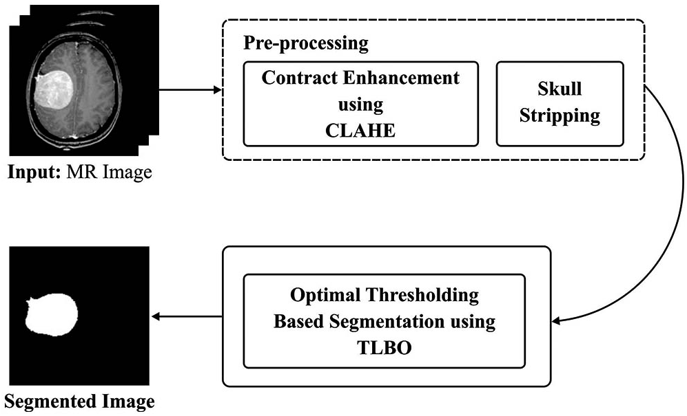
Figure 1: Overview of proposed method

2.1 Preprocessing

2.1.1 Contrast Limited Adaptive Histogram Equalization

Enhancement using contrast limited adaptive histogram equalization (CLAHE) prevents the distortion of the echo. The number of high-intensity histograms is determined using CLAHE [17]. Each histogram reflects various regions of the image. Intensity values are marked on maps using a shared histogram [18]. Low-contrast images are improved using CLAHE, as follows:

•   Derive total inputs: The input data are the number of rows and columns in the image. The number of bins of histograms is used to create the image mapping. Clip restrict is used to restrict the contrast (normalized from zero to one).

•   Preprocess inputs: The contrast rate is processed to determine the exact clip restrict if needed. The image is padded prior to segregation.

•   Process each contextual area to generate mappings with gray level: A small part of the image is taken; the histogram area is prepared using several bin calculations. The histogram is clipped using clip restrict, and the function is mapped for the particular area.

•   Interpolate gray level mappings to gather the last CLAHE image: Image regions are extracted from four clusters using the neighboring transformation function, and checked for partial overlaps of the transformation area. The pixels of the overlapped area are removed, and this process is repeated until all overlapping pixels are removed.

2.1.2 Skull Stripping

Stripping the skull is the first step in the segmentation of brain MRI images. This is necessary, as quantitative diagnosis requires extraction of the skull image from the background of the brain MRI. Skull stripping is accomplished with an image filter [19], which uses a masking technique to isolate parts of the image and differentiate pixels of equal intensity. The threshold value of a skull or bone MRI image will be greater than 200 compared to the tumor or other portion of the brain, and considering the threshold of the image being filtered. The skull picture is derived using the notion of solidity [20].

2.2 BTLBO Algorithm

2.2.1 TLBO Algorithm

Teaching-learning is essential to the algorithm’s progress, and may be compared to individual learning. The TLBO algorithm uses two simple models: teaching as an instructor and learning as a student [21]. The population refers to the set of students, and the problem of optimization is student usability. Optimal outcomes are referred to as instructors. The algorithm’s approach is defined from the perspectives of a teacher and student.

Teacher Phase: This stage follows the learning process via the instructor, whose role is to convey knowledge to students and make an effort to increase the average score of the class. Let m be the number of subjects that n students have accessed (i.e., population size, k = 1, 2,…, n). Mv,u is the mean performance of the students in a particular subject v (v = 1, 2,…, m) in some order of the teaching-learning process. A nominee from the ideal community acts as an instructor, who should have experience and skills. It is assumed that Atotal,kbest,u is the result of the optimal learner, assuming every subject is recognized as a teacher for that cycle. The instructor makes the greatest effort to increase the amount of data to cover the entire class. The final performance depends on the quality of the teacher’s delivery and a student’s learning capacity. The mean difference in the performance of the teacher and student in all subjects is

Difference_Meanv,u=ru(Av,kbest,u−THFMv,u), (1)

where Av,kbest,u is the teacher output (i.e., the optimal student) in subject v. THF is the teaching factor, which selects the mean value that must be changed, and ru is an arbitrary count in [0, 1]. THF can take the value 1 or 2, and is determined randomly as

THF=round[1+rand(0,1){2−1}], (2)

where rand is an arbitrary number in [0, 1]. THF is not related to the TLBO technique.

The value of THF is not given as an input in this method and is randomly chosen using Eq. (2).

The result based on the Difference_Meanv,u, in the teaching phase is

Av,k,u′=Av,k,u+Difference−Meanv,u, (3)

where, Av,k,u′ is the modified value of Av,k,u. Av,k,u′ is accepted when it gives the best function value. This can be a final function value of the teaching phase, and it becomes the input to the student phase.

The TLBO technique acts based on the values of ru, which is an arbitrary number in [0, 1], and the teaching factor THF. These are generated randomly. (Separate crossover and mutation are possible in the genetic algorithm (GA), inertia weight and cognitive and social parameters are possible in particle swarm optimization (PSO), and colony size and limits are possible in the artificial bee colony (ABC) algorithm). Hence it is not necessary to adjust ru and THF [22–24]. General parameters, such as the population size and number of generations, must be tuned and controlled. These are optimized for the entire population.

Learner Phase: This phase is inspired by the learning of learners. This occurs when one learner has more information than another, and is accomplished through interaction and discussion {[25,26]}. The learning process is as follows.

Two students P and Q are randomly selected so that Atot−P,u′≠Atot−Q,I′, where Atot−P,u′ and Atot−Q,u′ are the upgraded values of Atot−P,u and Atot−Q,u, respectively, at the final stage of the teaching phase.

Av,P,u″=Av,P,u′+ru(Av,P,u′−Xv,Q,u′),If Atotal−P,u′>Atotal−Q,u′, (4a)

Av,P,u″=Av,P,u′+ru(Av,Q,u′−Av,P,u′),If Atotal−Q,I′>Atotal−P,u′. (4b)

The above equations are for maximization problems; the reverse is true for minimization problems. Av,P,u″ is accepted only when it satisfies the optimal fitness value.

2.2.2 BTLBO with Boosted Learning

The outcome of the TLBO algorithm is enhanced either by learning from the teacher or other learners. Learners can also be boosted by enhancing their information capacity. The BTLBO technique determines the boosting phase for managing the information [27], which explains the TLBO and BTLBO techniques and the results of the teacher and learner phases. Duplicate results are randomly changed at the duplicate removal stage. Thus, for the TLBO process,

The total number of estimation functions ={(2×population size×number of generations)+(function evaluations required for duplicate elimination)}.

This study includes calculations of the total number of function estimations, using the above formula, for the TLBO and BTLBO techniques.

The flowchart for the BTLBO algorithm is shown in Fig. 2. The steps are as follows.

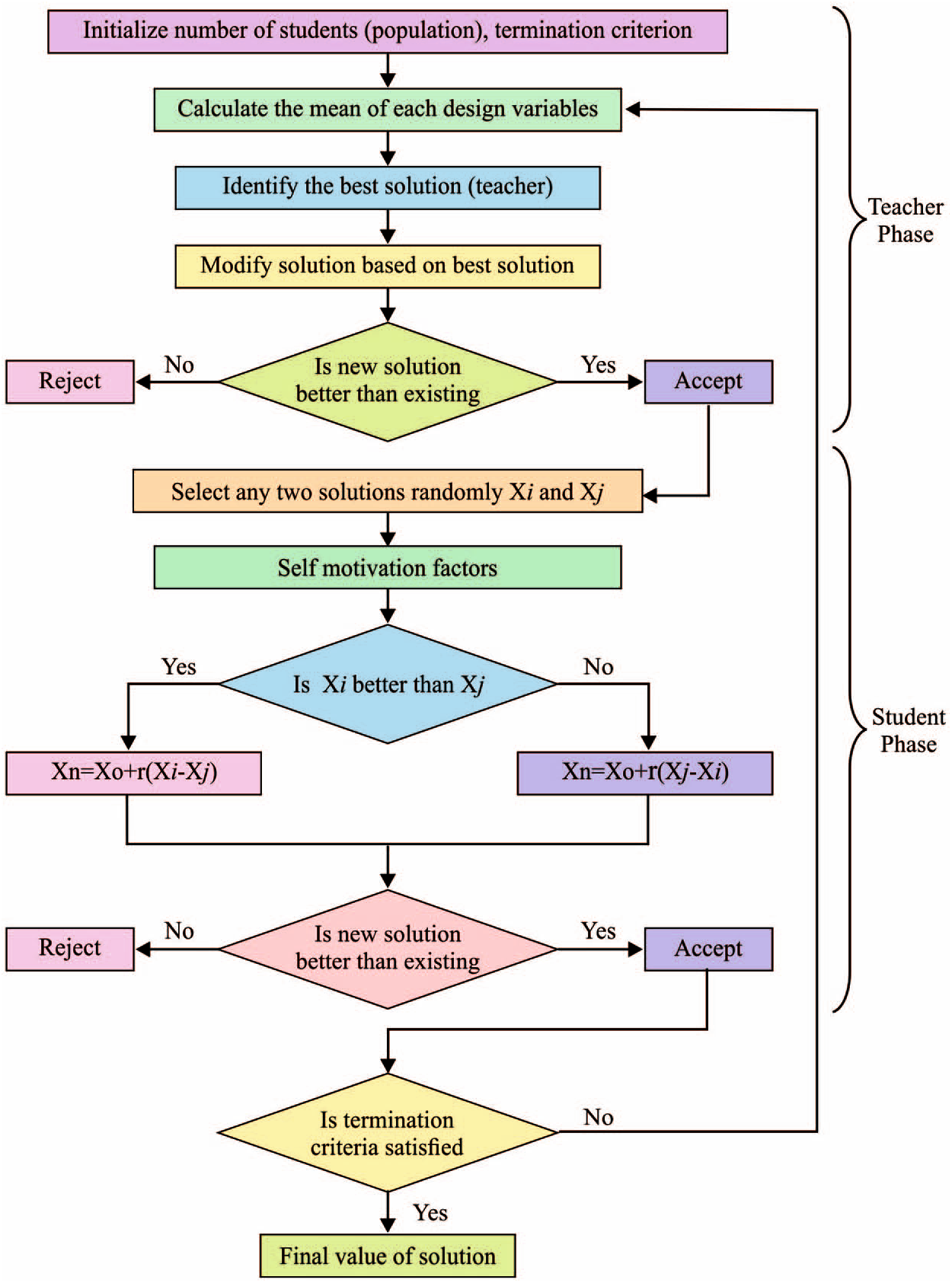
Figure 2: Flowchart of BTLBO algorithm

Step 1: Define the optimization problem as the minimization or maximization of f(A), which is the value of the objective function, where A is the design parameter vector.

Step 2: Initiate and assess the population initiation (i.e., learner, k=1,2,…,n, and subjects, v=1,2,…,m).

Step 3: Select the best solution as the teacher, and ranked as first for the process (i.e., f(A)best),

(Ateacher)1=f(A)1where f(A)1=f(A)best.

Step 4: Select the teacher according to the key rank,

f(A)s=f(A)1−rand∗f(A)1s=2,3,…,TH.

(When the values are unequal, choose the value of f(XA)s that is nearest to the computed value.)

(Ateacher)s=f(A)s,where s=2,3,…,TH.

Step 5: Allocate learners to the teacher according to the fitness value:

For k=1:(n−s),

If f(A)1≥f(A)k>f(A)2, assign the learner f(A)k to teacher 1 (i.e., f(A)1).

If f(A)2≥f(A)k>f(A)3,

allocate learner f(A)k to teacher 2 (i.e., f(A)2).

If (A)TH−1≥f(A)k>f(A)TH,

allocate learner f(A)k to teacher TH−1 (i.e., f(A)TH−1).

Else,

allocate learner f(A)k to teacher TH.

End

Step 6: Maintain the best solution for each set of functions.

Step 7: Determine the average result of the entire set of learners and subjects (i.e., (Mv)s).

Step 8: Determine the difference between the outcomes of teachers in every set of subjects through an adaptive teaching factor while keeping the respective average as a benchmark,

(Difference_Meanv)s=rand(Av,teacher−THFMv)s

s=1,2,…,TH,v=1,2,…,m.

Step 9: Based on the knowledge of the teacher, enhance the knowledge of the learner in every set along with the factor of tutorial hours,

(Av,k′)s=(Av,k+Difference−Meanv)s+rand(Ahh−Ak)s,If f(A)hh>f(A)k,

(Av,k′)s=(Av,k+Difference−Meanv)s+rand(Ak−Ahh)s,If f(A)k>f(A)hh,

where hh≠k.

Step 10: In the learner phase, update the knowledge of the learner along with other knowledge of learners if they are boosted,

(Av,k″)s=Av,k,u′+rand(Av,k′−Av,p′)s+rand(Ateacher−EFAv,k′)s,If f(Ak′)>f(Ap′),

(Av,k″)s=Av,k,u′+rand(Av,p′−Av,k′)s+rand(Ateacher−EFAv,k′)s,If f(Ap′)>f(Ak′),

where EF= exploration factor = round (1+ rand).

Step 11: Replace the existing poor solution with the obtained optimal solution.

Step 12: Randomly eliminate redundant solutions.

Step 13: Integrate all the sets.

Step 14: Repeat Steps 3 to 13 until the termination criteria are satisfied.

3  Experimental Validation

Fig. 3 shows sample visualization results from P-BTLBO. A sample set of test input images, contrast-enhanced images, skull stripped images, and segmented images are shown in Figs. 3a–3d, respectively.

Figure 3: Sample visualization results. (a) Original image; (b) Contrast enhanced image using CLAHE; (c) Skull stripped image; (d) Segmented image

The mean squared errors (MSE) of different models for a collection of pictures are shown in Tab. 1 and Fig. 4.

The P-BTLBO model achieved the best MSE of 11.87 for image 1, compared to 20.78 and 18.25, respectively, for GA and PSO. The PSO model yielded the minimum MSE, 14.73, for image 2, while GA and PSO had values of 19.25 and 16.23, respectively. P-BTLBO produced the minimum, at 15.94, for image 3, and GA and PSO had values of 20.35 and 18.26, respectively. P-BTLBO had the smallest value, 19.48, for image 4, while GA and PSO had values of 23.89 and 20.46, respectively. P-BTLBO achieved the smallest MSE, 15.97, for image 5, and the MSE values using GA and PSO were 24.20 and 20.31, respectively. P-BTLBO had the smallest MSE, 13.96, for image 6, while GA and PSO had values of 21.36 and 20.39, respectively. P-BTLBO generated an MSE of 15.42 for image 7, and GA and PSO returned values of 22.83 and 20.98, respectively. P-BTLBO had the smallest MSE, 16.31, for image 8, while GA and PSO had values of 26.28 and 23.45, respectively. P-BTLBO had the minimum MSE of 15.90 for image 9, and GA and PSO had values of 22.37 and 20.13, respectively. P-BTLBO produced the smallest MSE, 8.35, for image 10, and GA and PSO yielded values of 24.46 and 22.37, respectively.

Table 1: MSE analysis of various models

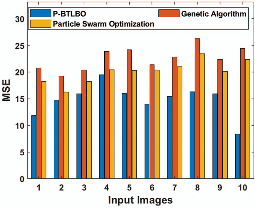
Figure 4: Comparative MSE analysis of different algorithms

Peak signal-to-noise ratio (PSNR) tests of different models for a series of pictures are shown in Tab. 2 and Fig. 5. P-BTLBO achieved a maximum PSNR value of 37.386 on image 1, while GA and PSO had values of 34.954 and 35.517, respectively. P-BTLBO achieved the best PSNR values on the other images, with an average PSNR value of 36.421, while GA and PSO had average values of 34.612 and 35.124, respectively.

Table 2: PSNR (dB) analysis of different algorithms

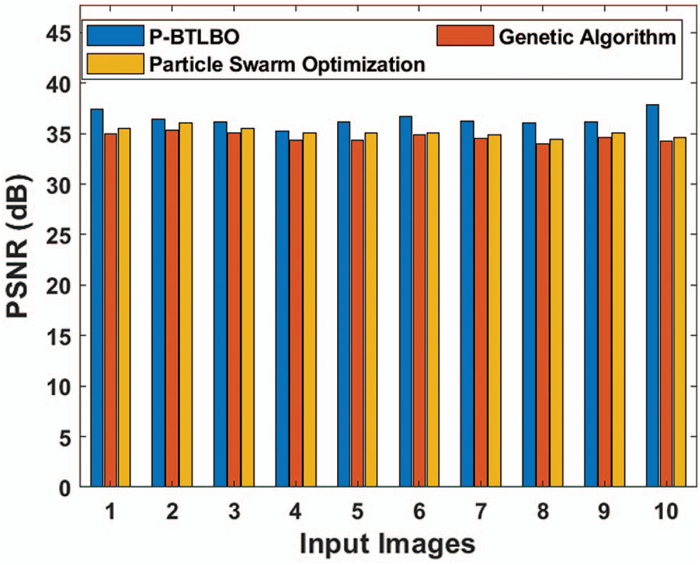
Figure 5: Comparative PSNR analysis of different algorithms

The findings from the study of the detection accuracy of various models are shown in Tab. 3 and Fig. 6. For image 1, the detection accuracy of P-BTLBO was best at 96.42, while GA and PSO produced values of 93.24 and 95.43, respectively. The DA value for image 2 using P-BTLBO was 97.29, and GA and PSO had values of 94.26 and 96.43, respectively. P-BTLBO had a DA value of 97.23 for image 3, while GA and PSO yielded values of 94.10 and 96.33, respectively. P-BTLBO provided a DA value of 96.85 for image 4, and GA and PSO had values of 93.58 and 95.24, respectively. P-BTLBO achieved a DA of 96.89 for image 5, while GA and PSO had values of 94.33 and 96.17, respectively. P-BTLBO achieved the best DA value, 95.83, for image 6, while GA and PSO had values of 94.239 and 95.38, respectively. P-BTLBO had a DA value of 95.94 for image 7, while GA and PSO yielded values of 94.23 and 95.90, respectively. P-BTLBO had a DA value of 95.34 for image 8, while GA and PSO had values of 93.40 and 95.25, respectively. P-BTLBO had a DA value of 96.85 for image 9, and GA and PSO had values of 94.60 and 96.35, respectively. P-BTLBO had a DA value of 95.31 for image 10, and GA and PSO had values of 93.59 and 94.29, respectively. The proposed P-BTBO algorithm produced superior results on average, with a DA of 96.39.

Table 3: Detection accuracy (DA) (%)

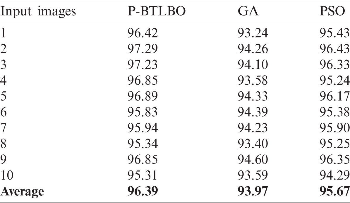
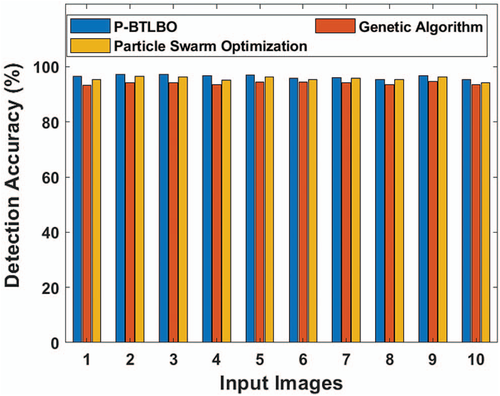
Figure 6: Comparative DA of different algorithms

4  Conclusion

This study introduced the P-BTLBO algorithm for automatic brain tumor segmentation in MRI images. Two preprocessing techniques were used for contrast enhancement and skull stripping. The classic TLBO algorithm was improved using a boosting mechanism. The BTLBO algorithm was tested on different photos. The proposed model greatly outperformed other models in simulations. The P-BTLBO algorithm showed superior results in experiments, reaching the highest accuracy (96.39%), with an average PSNR value of 36.421dB. P-BTLBO algorithm showed more promising experimental results in automated segmentation than the GA and PSO algorithms. The model presented in this study may be extended in the future to the extraction and classification of features.

Acknowledgement: We thank LetPub (www.letpub.com) for its linguistic assistance during the preparation of this manuscript.

Funding Statement: The author(s) received no specific funding for this study.

Conflicts of Interest: The authors declare that they have no conflicts of interest to report regarding the present study.

This work is licensed under a Creative Commons Attribution 4.0 International License, which permits unrestricted use, distribution, and reproduction in any medium, provided the original work is properly cited.