Computers, Materials & Continua DOI:10.32604/cmc.2021.017225
Article

GPS Vector Tracking Loop with Fault Detection and Exclusion

Dah-Jing Jwo*and Meng-Hsien Hsieh

Department of Communications, Navigation and Control Engineering, National Taiwan Ocean University, Keelung, 202301, Taiwan
*Corresponding Author: Dah-Jing Jwo. Email: djjwo@mail.ntou.edu.tw
Received: 19 January 2021; Accepted: 24 February 2021

Abstract: In this paper, both the integrity monitoring and fault detection and exclusion (FDE) mechanisms are incorporated into the vector tracking loop (VTL) architecture of the Global Positioning System (GPS) receiver for reliability enhancement. For the VTL, the tasks of signal tracking and navigation state estimation no longer process separately and a single extended Kalman filter (EKF) is employed to simultaneously track the received signals and estimate the receiver’s position, velocity, etc. In contrast to the scalar tracking loop (STL) which utilizes the independent parallel tracking loop approach, the VTL technique is beneficial from the correlation of each satellite signal and user dynamics. The VTL approach provides several important advantages. One of the merits is that the tracking loop can be assisted for overcoming the problem of signal blockage. Although the VTL architectures provide several important advantages, they suffer some fundamental drawbacks. For example, the errors in the navigation solutions may degrade the tracking accuracy. The most significant drawback is that failure of tracking in one channel may affect the entire tracking loop and possibly lead to loss of lock. For reliability enhancement, the EKF based integrity monitoring and FDE algorithms are developed to prevent the error from spreading into the entire tracking loop. The integrity monitoring is utilized to check the possible fault in the pseudorange and the pseudorange rate, followed by the FDE mechanism employed to exclude the abnormal satellite signals. Performance assessment and evaluation for the proposed approach will be presented.

Keywords: Global Positioning System; vector tracking loop; signal blockage; integrity; fault detection and exclusion

1  Introduction

The Global Positioning System (GPS) is a satellite-based navigation system [1–5] that provides a user with the proper equipment access to useful and accurate positioning information anywhere on the globe. Generally, the GPS receiver accomplishes the following two major functions: (1) tracking of the pseudorange and pseudorange rate, and (2) solving the navigation states. The signal tracking tries to adjust the local signal to synchronize the code phase with the received satellite signal. Traditional GPS receivers track signals from different satellites independently where each tracking channel measures the pseudorange and pseudorange rate, respectively, and then sends the measurements to the navigationF processor to solve for the user’s position, velocity, clock bias and clock drift (PVT).

As the most vulnerable parts of a receiver, the carrier and code tracking loops play a key role in a GPS receiver. The scalar tracking loop (STL) processes signals from each satellite separately. Specifically, a delay lock loop (DLL) is adopted to track the code phase of the incoming pseudorandom code and a carrier tracking loop, such as a frequency lock loop (FLL) or a phase lock loop (PLL), is adopted to track the carrier frequency or phase. The tracking results from different channels are then combined to perform the navigation state estimate. The drawback of a STL is that it neglects the inherent relationship between the navigation solutions and the tracking loop status. A STL is more like an open loop system and suffered from performance degradation when scintillation, interference, or signal outages occur. The vector tracking loop (VTL) [6–11] provides a deep level of integration between signal tracking and navigation solutions in a GPS receiver and possesses significant important improvement over the traditional STL. The notable advantages of the VTL include the increase of interference immunity, the ability to operate at low signal power and bridge short signal outages, and the robust dynamic performance. Although the current VTL architectures provide several important advantages, they suffer some fundamental drawbacks. The errors in the navigation solutions may degrade the accuracy of the tracking loop results. Furthermore, the failure of tracking in one channel may affect the entire system and lead to loss of lock on all satellites. To ensure a user position solution with predetermined uncertainty levels, reliability monitoring and assessment are important.

Navigation system integrity refers to the ability of the system to provide timely warming to users when the system should not be used for navigation. It is regarded as a risk factor can provide timely warning to users when the position error exceeds a specified limit. The receiver autonomous integrity monitoring (RAIM) [12–17] was proposed in the latter half of the 1980’s. A variety of RAIM schemes have been proposed based on some kind of self-consistency check among the available redundant measurements. The conventional RAIM is based on the snapshot approach which assumes each measurement is uncorrelated from one minute to the next. With this method, only current redundant measurements are used in the self-consistency check. The instantaneous snapshot least squares residual vector is used to compute the test static. The principle is based on the use of redundant satellite observations (redundant message) by mutual checking of data consistency (consistency check) to detect whether the satellite signals to provide the correct information. Reliability monitoring typically consists of testing the residuals of the observations statistically on an epoch-by-epoch basis with the aim of detecting and excluding measurement errors and, therefore, obtaining consistency among the observations with assigned uncertainty levels.

In addition to the least squares method, the sequential approach that uses the extended Kalman filter (EKF) [18,19] can be employed for processing of navigation solution and integrity monitoring. The well-known Kalman filter provides optimal (minimum mean square error) estimate of the system state vector and has been widely applied in many engineering applications. The Kalman filter is a recursive filter, for which there is no need to store past measurements for the purpose of computing present estimates. Given a signal that consists of a linear dynamical system driven by stochastic white noise processes, the Kalman filter provides a method for constructing an optimal estimate of the system state vector. While employed in the GPS receiver as the navigational state estimator, the EKF has been one of the promising approaches as an alternative method for integrity monitoring. In this paper, the EKF based integrity monitoring and FDE algorithms are incorporated to prevent the error of one channel from spreading into the entire tracking loop.

The remainder of this paper is organized as follows. In Section 2, preliminary background on system model for the GPS vector tracking loop is reviewed. The snapshot approach for GPS navigation solution with RAIM is introduced in Section 3. The EKF based integrity monitoring and FDE algorithms are discussed in Section 4. In Section 5, simulation experiments are carried out to evaluate the performance for various scenarios. Conclusions are given in Section 6.

2  System Model for the GPS Vector Tacking Loop

The traditional GPS receiver involves some parallel DLLs, each of which tracks a satellite to estimate the corresponding pseudorange. The parallel pseudorange measurements are sent to the navigation filter to solve for the navigation state vector. The VTL differs from the traditional STL in that the task of navigation solutions, code tracking and carrier tracking loops for all satellites are combined into one loop. The central part of a VTL is the EKF which provides an optimal estimation of signal parameters for all satellites in view and user PVT solutions based on both current and previous measurements from all satellites.

In the VDLL, each channel does not form a loop independently. The vector comprised of outputs of all the code phase discriminators is the measurement of navigation filter. The navigation state vector is estimated by navigation filter, and the error signals arise from the estimated user positions and the satellite positions calculated by the ephemeris. The code loop numerically-controlled oscillator (NCO) as the signal generator in the SDLL is replaced by the estimated user positions, to control the update of the local code. When one channel experiences interference or signal outages in the VTL, the information from other satellites can be used estimate the status of this channel. The system architectures for the STL and VTL are shown as in Fig. 1. The integrity check algorithms are used to detect the possible error in each channel to prevent the spreading of the error.

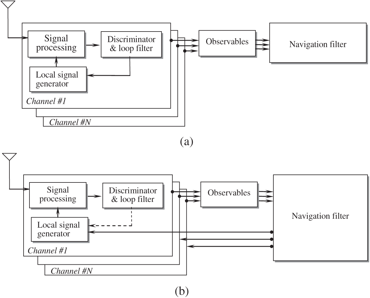
Figure 1: The system architectures for (a) scalar tracking loop and (b) vector tracking loop

The code phase observation of the GPS C/A code can be represented by:

ρ=1λC/A(r+δr+cδt)+ε(1)

where λC/A is the GPS C/A code wavelength; r and δr represent the range and its change between receiver antenna and GPS satellite; c is the speed of light; δt is the receiver clock offset; ε is the error term which includes the ionosphere delay, troposphere delay, measurement noise errors and multi-path errors etc. In order to remove the sensitivity on the variation of the signal amplitude and the reinforce on the track loop lock, the normalized energy difference between early and late code is selected as code loop phase discriminator.

δρ=(IE2+QE2)-(IL2+QL2)(IE2+QE2)+(IL2+QL2)(2)

In Eq. (2), the correlated outputs that the early and late In-phase/quadrature phase values can be calculated as follows

IE=2(C/N0)TR(Δτ+d2) sinc(δfT)cos(δφ)+ηIEQE=2(C/N0)TR(Δτ+d2) sinc(δfT)sin(δφ)+ηQEIL=2(C/N0)TR(Δτ-d2) sinc(δfT)cos(δφ)+ηILQL=2(C/N0)TR(Δτ-d2) sinc(δfT)sin(δφ)+ηQL

where C/N0 is the carrier to noise ratio of the received signal, R denotes the code correlation functions with correlator spacing d (≤1) [chip], δτ is the code delay error, δφ is the carrier phase error, δf is the Doppler shift error, η is the independent in-phase component and orthogonal component of the Gaussian Noise. The cross-correlation function between local prompt code and the received spreading code is

R(τ)={1-|τ|0|τ|≤1|τ|>1(3)

where τ is in unit of chip. In the ideal case with noise, when the spacing between early and late code is one chip, and the input error range is ±0.5 chips, the output of phase discriminator is equal to the tracking error.

3  The Snapshot Approach for GPS RAIM

Consider the vectors relating the Earth’s center, satellites and user positions. The vector s represents the vector from the Earth’s center to a satellite, u represents the vector from the Earth’s center to the user’s position, and r represents the vector from the user to the satellite. The vector relation can be obtained

r=s-u(4)

The distance ||r|| is computed by measuring the propagation time from the transmitting satellite to the user/receiver. The GPS pseudorange ρi is defined for the i th satellite by

ρi=||si-u||+ctb+vρi(5)

where c is the speed of light and tb is the receiver clock offset from system time, and vρi is the range noise. Consider the user position in three dimensions, denoted by (xu,yu,zu), the pseudorange observables made to the n satellites can be written as

ρi=(xi-xu)2+(yi-yu)2+(zi-zu)2+ctb+vρi,i=1,…,n(6)

where (xi,yi,zi) denotes the i -th satellite’s position in three dimensions.

3.1 Linearization of the GPS Pseudorange Equations

The states and the measurements are related nonlinearly; the nonlinear ranges are linearized around an operating point using Taylor’s series. Eq. (6) can be linearized by expanding Taylor’s series around the approximate (or nominal) user position (x^n,ŷn,ẑn) and neglecting the higher-order terms. Defining ρ^i as ρi at (x^n,ŷn,ẑn) we have

Δρi=ρi-ρ^i=ei1Δxu+ei2Δyu+ei3Δzu+ctb+vρi(7)

where

ei1=x^n-xir^i;ei2=ŷn-yir^i;ei3=ẑn-zir^ir^i=(x^n-xi)2+(ŷn-yi)2+(ẑn-zi)2(8)

The vector (ei1,ei2,ei3)≡Ei, i=1,…,n, denotes the line-of-sight vector from the user to the satellites. Eq. (7) can be written in a matrix formulation

Δρ=[Δρ1Δρ2Δρ3⋯Δρn]T=[e11e12e131e21e22e231e31e32e331⋮⋮⋮⋮en1en2en31][δxuδyuδzuctb]+vρ(9)

which can be represented as

y=Gx+ε(10)

The matrix G has the dimension of n×4 with n≥4, and is usually referred to as the ‘geometry matrix’ or ‘visibility matrix.’ The instantaneous “snapshot” approach assumes that each measurement is uncorrelated from one minute to the next time. The least-squares solution to Eq. (10) is given by

xLS=(GTG)-1GTy(11)

3.2 RAIM Based on Snapshot Approach

Navigation system integrity refers to the ability of the system to provide timely warning to users when the system should not be used for navigation. The conventional RAIM is usually the “snapshot” type of approaches. While four satellites are sufficient for navigation, at least five satellites in view are needed for integrity monitoring. Otherwise, the geometry is unavailable for GPS RAIM. The linearized GPS pseudorange equation is an over-determined system of linear equations when the number of visible satellites is more than four. Three RAIM methods have received special attention in recent literatures on GPS integrity, including the range comparison method, least-squares residual method, and parity method. All three methods are snapshot schemes in that they assume that noisy redundant range-type measurements are available at a given sample point in time.

In the least-squares residuals method, the residuals are formed in much the same manner as was done in the range comparison method. Since the least-squares estimate of the solution is given by Eq. (11), the estimate of the measurement vector can be written as y^=Gx^LS=G(GTG)-1GTy. The range residual vector is defined as

w=y-y^==[In-G(GTG)-1GT]ε(12)

This is the liner transformation that takes the range measurement error into resulting residual vector. The sum of the squares of the elements of w is called the sum of squared errors (SSE).

SSE=wTw

The test statistic employed in the RAIM algorithm in terms of SSE is given by

TestStatistics=SSE/(n-4)(13)

where SSE is the unnormalized sum of the squared measurement residuals in all-in-view least squares solution and n is the number of satellites in view. When properly normalized, SSE has a Chi-square distribution with (n-4) degrees of freedom.

4  The EKF Based Approach for Integrity Monitoring and FDE Algorithms

In addition to the sequential approach, the other method is referred to as the sequential algorithm, where the Kalman filter is commonly employed. The approach is sometimes referred to as the Autonomous Integrity Monitored Extrapolation (AIME). The Kalman filter algorithms used in the linear system can be extended to the nonlinear system via the EKF approach, which is a nonlinear version of the Kalman filter and is widely used for the position estimation in GPS receivers. The process model and measurement model for the EKF can be written as

xk+1=f(xk)+wkzk=h(xk)+vk

where the state vector xk∈ℜn, process noise vector wk∈ℜn, measurement vectorzk∈ℜm, and measurement noise vector vk∈ℜm. Both the vectors wk and vk are zero mean Gaussian white sequences having zero crosscorrelation with each other:

E[wkwiT]={Qk,i=k0,i≠k;E[vkviT]={Rk,i=k0,i≠k;E[wkviT]=0foralliandk where E[⋅] represents expectation, and superscript “T” denotes matrix transpose, Qk is the process noise covariance matrix, Rk is the measurement noise covariance matrix.

The discrete-time extended Kalman filter algorithm is summarized as follow:

•    Correction steps/measurement update equations:

Kk=Pk-HkT[HkPk-HkT+Rk]-1 (14)

x^k=x^k-+Kk[zk-hk(x^k-)] (15)

Pk=[I-KkHk]Pk- (16)

•    Prediction steps/time update equations:

x^k+1-=fk(x^k) (17)

Pk+1-=ΦkPkΦkT+Qk (18)

Implementation of the EKF algorithm starts with an initial condition value, x^0- and P0-. When new measurement zk becomes available with the progression of time, the estimation of states and the corresponding error covariance would follow recursively ad infinity. The linear approximation equations for system and measurement matrices are obtained through the relations

Φk≈∂fk∂x|x=x^k-;Hk≈∂hk∂x|x=x^k-(19)

Further detailed discussion can be referred to Gelb [18] and Brown et al. [19].

4.1 Autonomous Integrity Monitored Extrapolation

The statistic s2 (sum of squared residuals, or simply SSR for short) is used to detect failure, in the way that the parity vector squared magnitude p2 is used in RAIM. If there are n satellites in view, s2 is Chi-square distributed with n degrees of freedom, and p2 is Chi-square distributed with n −4 degrees of freedom. This means that AIME can detect failures with as few satellites in view, while RAIM requires a minimum of five satellites with good geometry. The significant difference is that s2 depends on the entire past history of measurements.

When redundant observations have been made, Kalman filter residuals of the pseudoranges:

υk=zk-hk(x^k-)(20)

has zero mean, E[υk]=0, and residual covariance given by:

E[υkυkT]=Uk=HkPk-HkT+Rk(21)

Satellite failures are detected by using the magnitude of the normalized residual vector s as the test statistic:

s2=sTs=υkTUk-1υk(22)

In the process of failure detection, the threshold sD for detecting failures is Chi-square distributed with n degrees of freedom. It is selected to result in the false alarm rate. The probability density function associated with a Chi-square distributed with k degrees of freedom is

f(x)={2-k/2Γ(n/2)x(k/2)-1e-k/2ifx>00ifx≤0(23)

where Γ(x)=∫0∞tx-1e-tdt indicates the gamma function. The fault alarm rate (denoted as PFA) is defined as

PFA=∫a∞f(x)dx(24)

The parameter a is the normalized threshold for |s2| as the test statistic. Therefore the normalized threshold for |s| as the test statistic is a. It can be found that the threshold sD=σ⋅a, where σ is the standard deviation. When s≥sD, a “failure alarm” is reported; on the other hand, when s<sD, the GPS receiver is in normal condition, and no failure is reported.

4.2 Fault Detection and Exclusion (FDE)

After detecting the fault, it is helpful to find out the unhealthy satellites to be eliminated. The pseudorange residuals υk can be standardized as follows:

wi=|υkiUii|,i=1,2,3…,N(25)

where N denotes the number of observations. Each standardized residual wi is compared to the α0-quantile of the standardized normal distribution, n1-α0/2, with the predetermined false alarm rate α0 (PFA):

f(x)=12πexp(-x22)(26)

with the threshold of n1-α0/2.

∫0af(x)dx=1-α02(27)

The relative parameter n1-α0/2 and wi for fault detection has the following relationship:

{wi>n1-α0/2 Fault detectedwi≤n1-α0/2Nofaultdetected(28)

Fig. 2 shows the algorithm for implementing the GPS vector tracking loop with integrity monitoring and FDE mechanisms involved.

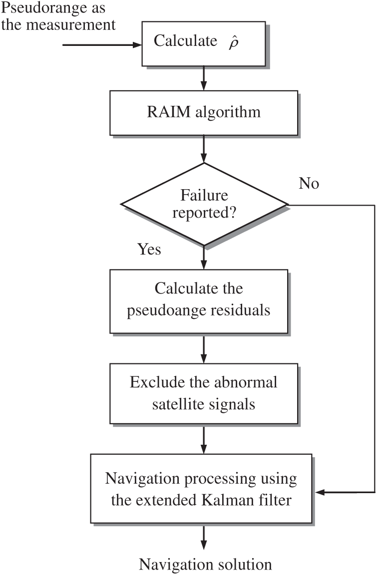
Figure 2: GPS vector tracking loop with integrity monitoring and FDE algorithms

5  Results and Discussion

Simulation experiments are carried out for confirmation of the effectiveness and performance evaluation of the proposed design. The computer codes were developed using the Matlab®; software. The commercial software satellite navigation toolbox (SATNAV) by GPSoft LLC [20] was employed. The simulation scenario is designed as follows. The experiment assumes a simulated vehicle trajectory originating from the position of North 25.1492 degrees and East 121.7775 degrees at an altitude of 100 m., which is equivalent to [-3042329.24911080.22694074.3]T m in the WGS-84 ECEF coordinate system. The location of the origin is defined as the (0,0,0) m location in the local tangent East-North-Up (ENU) frame. Shown in Fig. 3, the test trajectory can be divided mainly into several time intervals/segments according the various dynamic characteristics. The vehicle was simulated to conduct constant acceleration level flight during 0–25 s, clockwise circular motion with radius 750 m during 41–231 s, and counter-clockwise turn during 283–374 s, where high dynamic maneuvering is involved. For all the other segments, the constant-velocity straight-line flight is conducted. The skyplot is shown in Fig. 4. At the initial time of simulation, there are 9 satellites visible, each of which is numbered with a space vehicle identifier (SV ID).

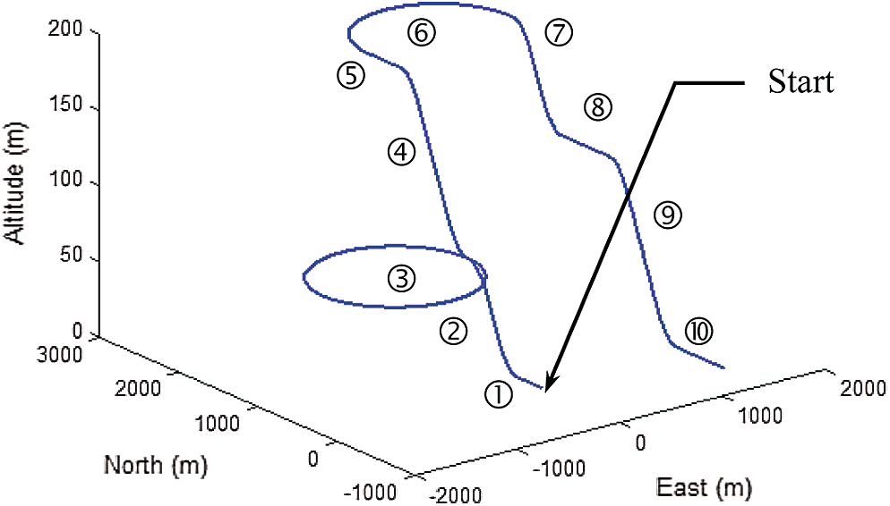
Figure 3: The test trajectory

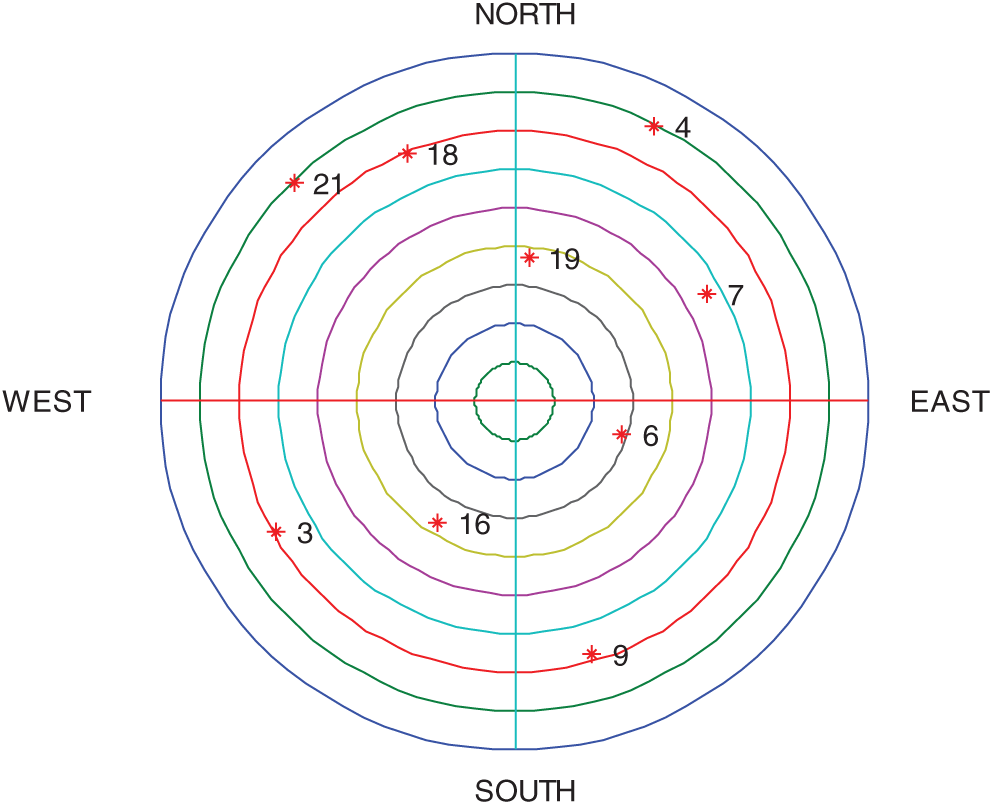
Figure 4: The skyplot at the initial time of simulation

When selecting extended Kalman filter as the navigation state estimator in the GPS receiver, using b and d to represent the GPS receiver clock bias and drift, the differential equation for the clock error is written as

ḃ=d+ubḋ=ud(29)

where ub~N(0,Sf) and ud~N(0,Sg) are independent Gaussianly distributed white sequences. The dynamic process of the GPS receiver in lower dynamic environment can be represented by the PV (Position-Velocity) model. In such case, we consider the GPS navigation filter with three position states, three velocity states, and two clock states, so that the state to be estimated is a 8×1 vector. The process model is given by

[ẋ1ẋ2ẋ3ẋ4ẋ5ẋ6ẋ7ẋ8]=[0100000000000000000100000000000000000100000000000000000100000000][x1x2x3x4x5x6x7x8]+[0u20u40u6u7u8] where x1, x3, x5 represent the east, north, and vertical position; x2, x4, x6 represent the east, north, and vertical velocity; and x7 and x8 represent the receiver clock offset and drift errors, respectively. The process noise covariance matrix is as follows:

Qk=[QeQnQuQt](30)

where

Qe=Qn=Qu=[SpΔt33SpΔt22SpΔt22SpΔt];Qt=[SfΔt+SgΔt33SgΔt22SgΔt22SgΔt]

If only the pseudorange observables are available, the linearized measurement equation based on n observables can be written as

[ ρ1ρ2⋮ρn ]−[ ρ^1ρ^2⋮ρ^n ]︸Zk=[hx(1)0hy(1)0hz(1)010hx(2)0hy(2)0hz(2)010⋮⋮⋮⋮⋮⋮⋮⋮hx(n)0hy(n)0hz(n)010]︸Hk[x1x2x3x4x5x6x7x8]+[vρ1vρ2⋮vρn](31)

where Hk is a matrix with dimension n×8. The measurement noise variances rρi are assumed a priori known, which is set as 9 m2. Let each of the white-noise spectral amplitudes that drive the random walk position states be Sp=1.0(m/s2)/rad/s. In addition, let the clock model spectral amplitudes be Sf=0.4(10-18)s and Sg=1.58(10-18)s-1. These spectral amplitudes can be used to find the Qk parameters in Eq. (30).

The scenarios involved in the numerical experiments cover two aspects. The first one deals with performance comparison for VTL and STL architectures for various numbers of visible satellites. The second one deals with reliability enhancement when the RAIM and FDE mechanisms are incorporated into the VTL.

5.1 Performance Comparison for VTL and STL Architectures

In the first part of experiment, performance comparison for VTL- and STL-based solutions is presented. Three examples, with good or bad geometry involved, are given to illustrate the effectiveness of the VTL architecture.

(1) Example 1: nine satellites visible

In the first example, it is assumed that all the GPS signals are in good condition. There are totally 9 GPS signals available in the open sky. Fig. 5 provides the comparison of code tracking errors for the 9 channels. As can be seen, the code tracking errors based on the VTL have been remarkably mitigated.

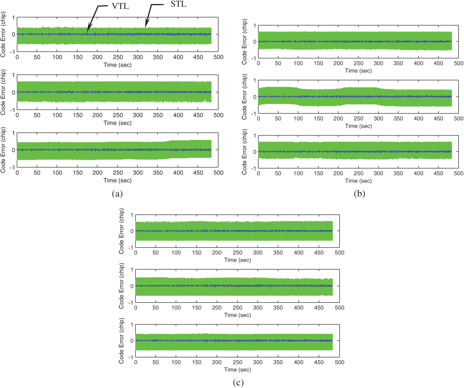
Figure 5: Comparison of code tracking errors for the 9 channels (a) channels 1–3 (b) channels 4–6 (c) channels 7–9

(2) Example 2: one out of five visible satellites blocked out at some time intervals

The second and third examples present the performance comparison in the case of signal blockage. Initially there are only 5 satellites visible, where some of the GPS signals are intentionally blocked out at some time intervals. In this example, we consider one signal is blocked out at certain time interval. Tab. 1 shows the time intervals during which signal blockage occurs. The symbol ‘✓’ indicates the signals that were blocked out at the time intervals as indicated. The code tracking errors for the five channels are shown in Fig. 6, where the gaps represent the discontinuities of signal reception. The VTL- and STL-based position errors are given in Fig. 7. It can be seen that the positioning accuracy based on the VTL has been effectively improved.

Table 1: Time intervals during which signal abnormalities occur for Example 2

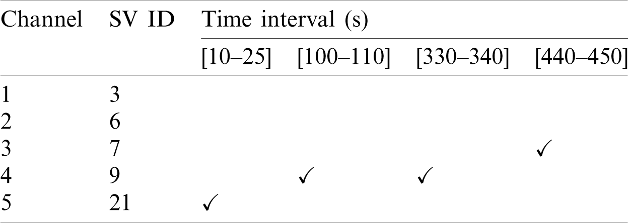
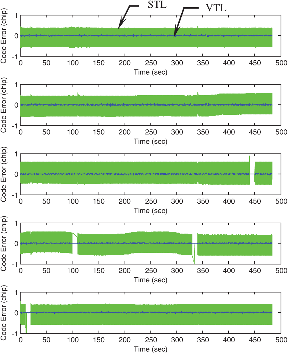
Figure 6: Code errors for the 5 channels

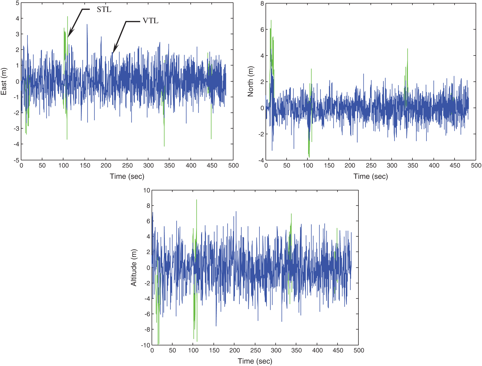
Figure 7: Comparison of position errors–VTL vs. STL

(3) Example 3: two out of five visible satellites blocked out at some time intervals

In this example, it is assumed that the number of visible satellites has been reduced from 5 to 3 at some time intervals. Same as in Example 2, there are initially 5 satellites visible. However, 2 GPS signals are blocked out simultaneously at some time intervals. Tab. 2 shows the time intervals during which two of the signals are blocked out. In such case, Fig. 8 provides the code errors for the five channels. The VTL and STL based position errors are given in Fig. 9. Since only three satellite signals are available at some time intervals, the performance degradation in the STL become more serious. It can be seen that the code tracking performance based on the VTL has been remarkably improved.

Table 2: Time intervals during which signal abnormalities occur for Example 3

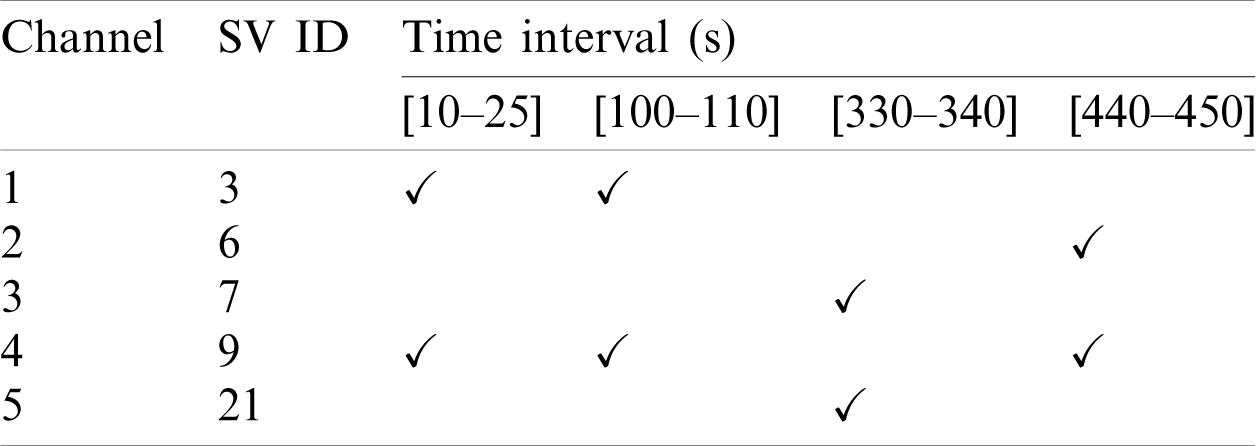
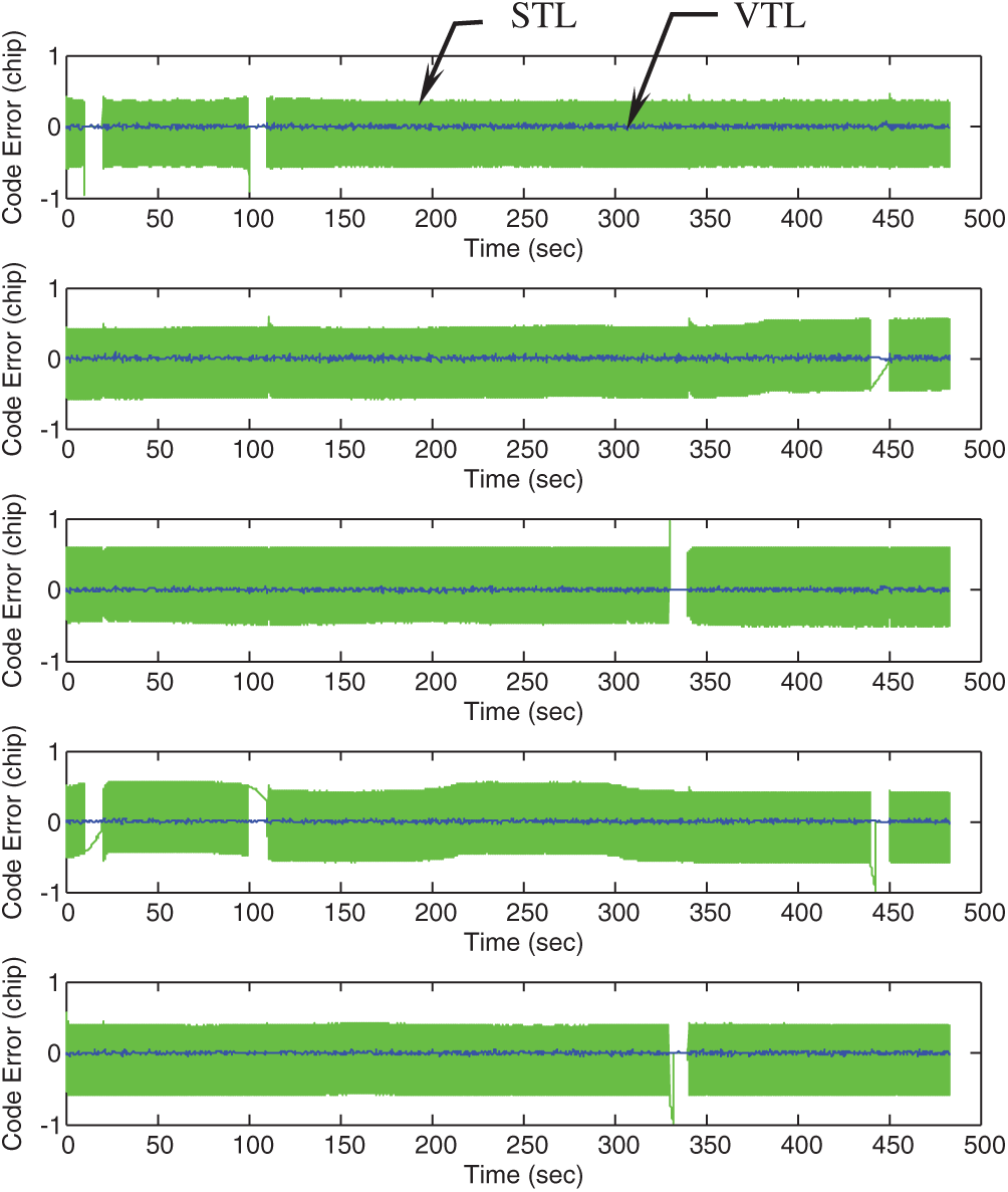
Figure 8: Code errors for the 5 channels

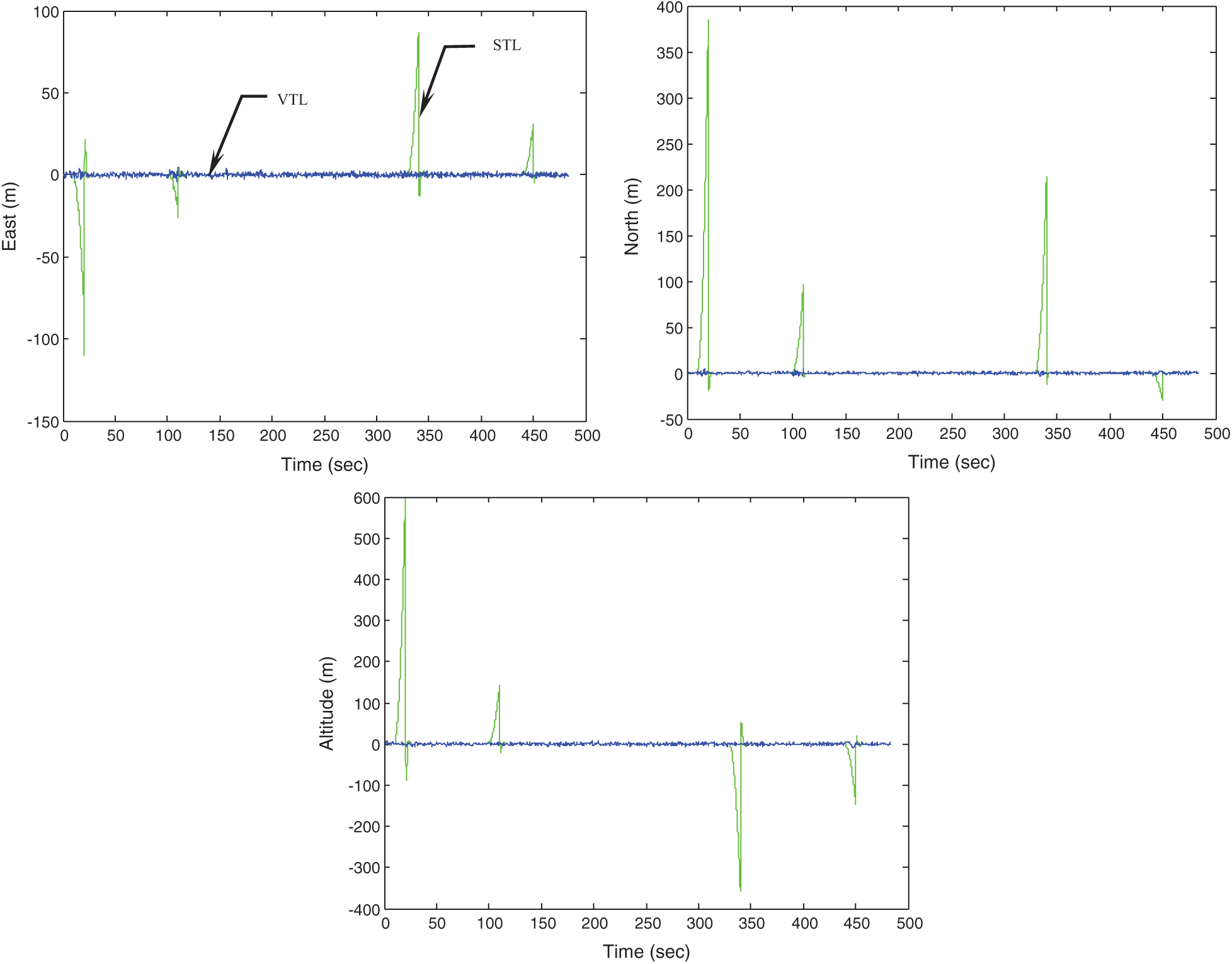
Figure 9: Comparison of positioning errors—VTL vs. STL

5.2 Performance Comparison for VTL with FDE Mechanism

In the second part of experiment, reliability enhancement for VTL using the FDE mechanism is presented. Two examples are given for illustration. It is assumed that there are 9 GPS signals available, but some fault signals occur at certain time interval.

(1) Example 1: one out of nine signals abnormal at some time interval

The abnormal signals corrupted by bias errors are assumed to occur at the following time intervals: 10–20 s, 220–230 s, 300–310 s, 370–380 s, and 440–450 s, as summarized in Tab. 3. The symbol ‘✓’ indicates the intervals where the signal abnormalities are involved. After excluding the faults, the performance improvement can be seen, as shown in Fig. 10. For example, in the time interval 220–230s, the signal fault in Channel 3 needs to be isolated. Fig. 11 shows the improvement on positioning accuracy with the assistance of FDE mechanism.

Table 3: Time intervals during which signal abnormalities occur for Example 1

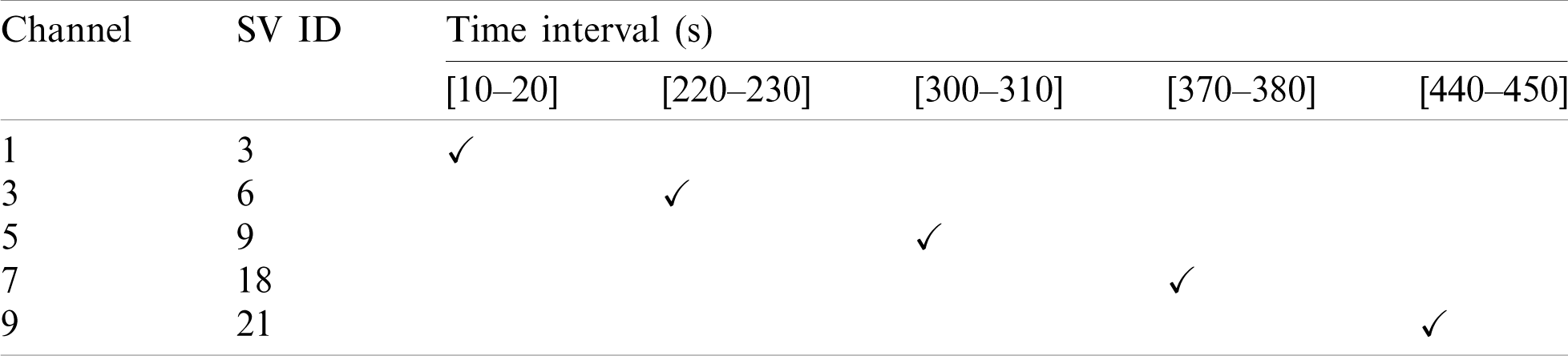
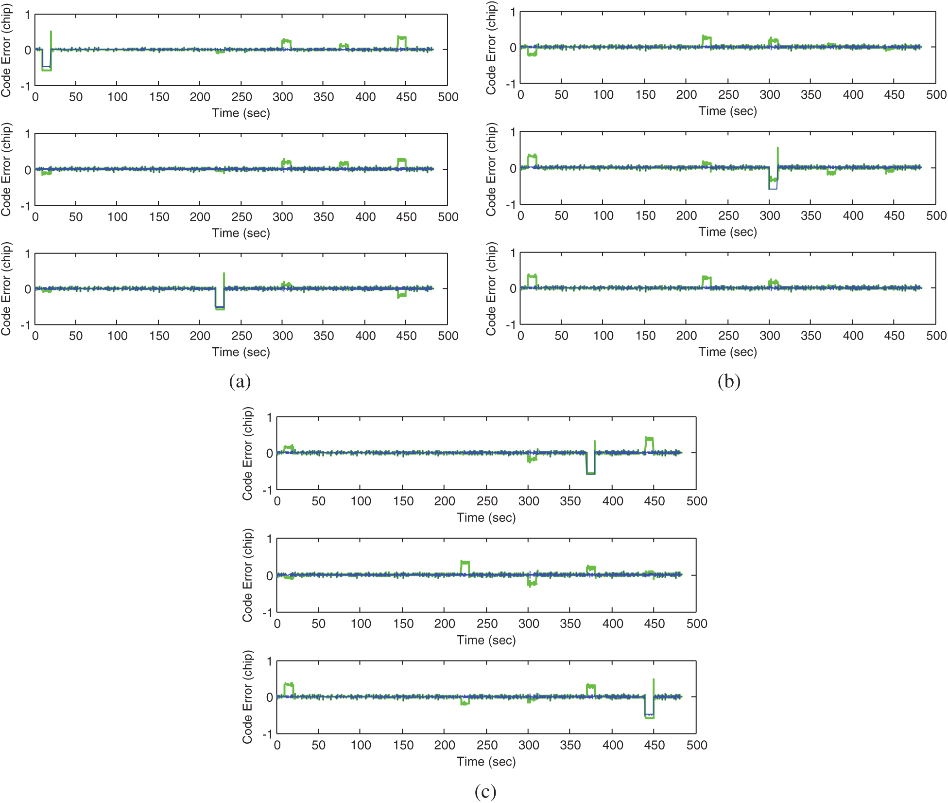
Figure 10: The code errors for the 9 channels (a) channels 1–3 (b) channels 4–6 (c) channels 7–9

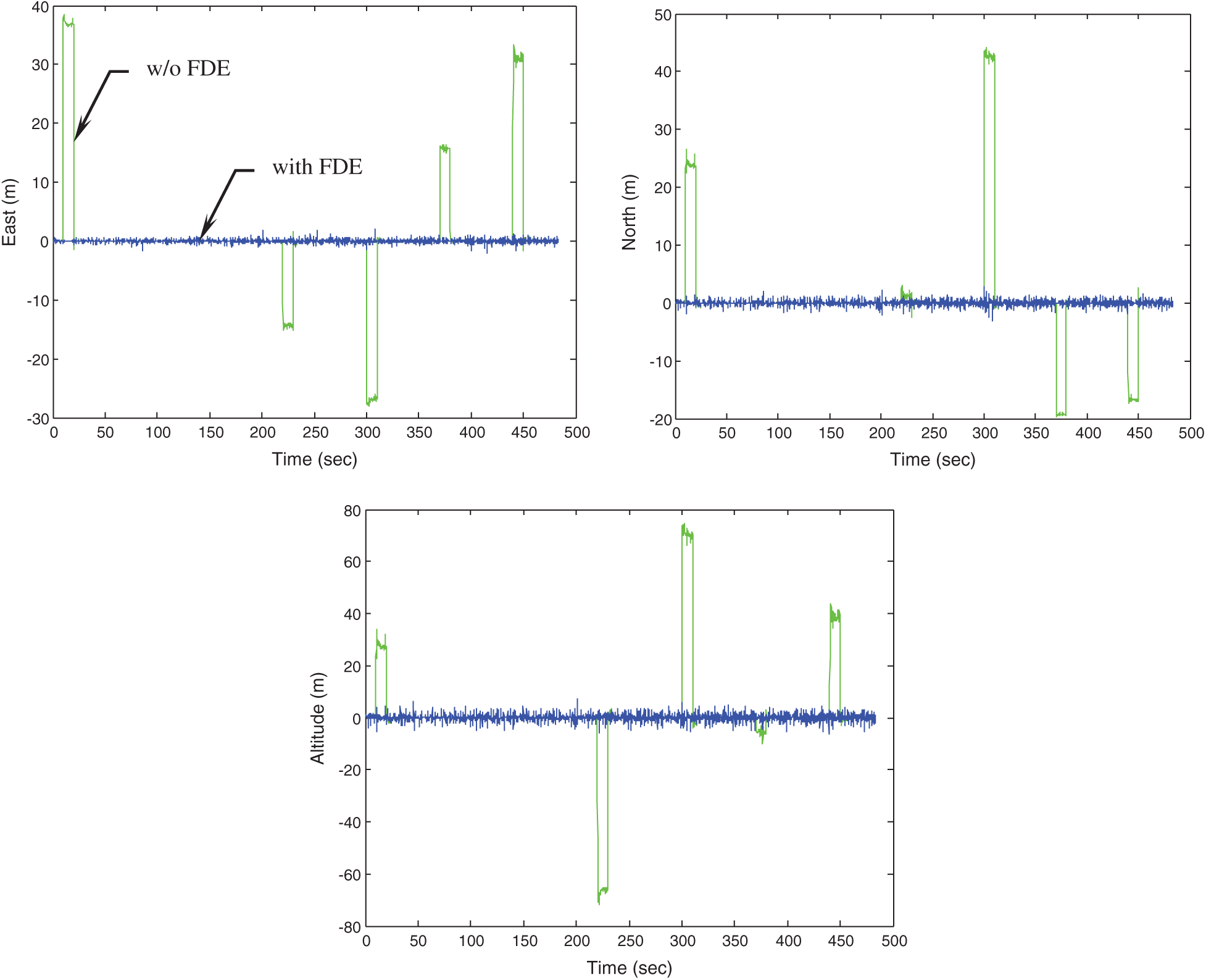
Figure 11: The positioning accuracy for the navigation algorithm with and without FDE mechanism

(2) Example 2: three out of nine signals abnormal simultaneously at some time intervals

The second example investigates the case when 3 abnormal signals occur simultaneously. Tab. 4 shows the time intervals during which signal abnormalities occur. Fig. 12 presents the position accuracy for the navigation algorithms with and without FDE. Once there are abnormalities in the GPS signals, the positioning performance are seriously degraded. Incorporation of the FDE algorithm has demonstrated remarkable improvement in navigation accuracy.

Table 4: Time intervals during which signal abnormalities occur for Example 2

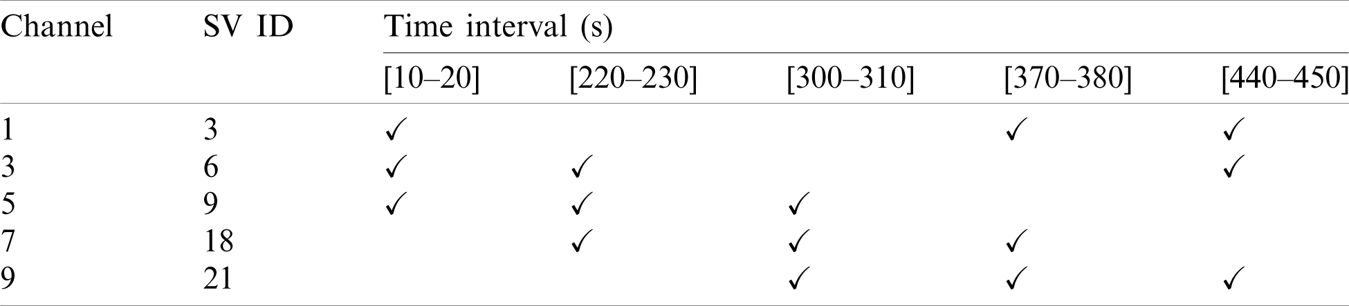
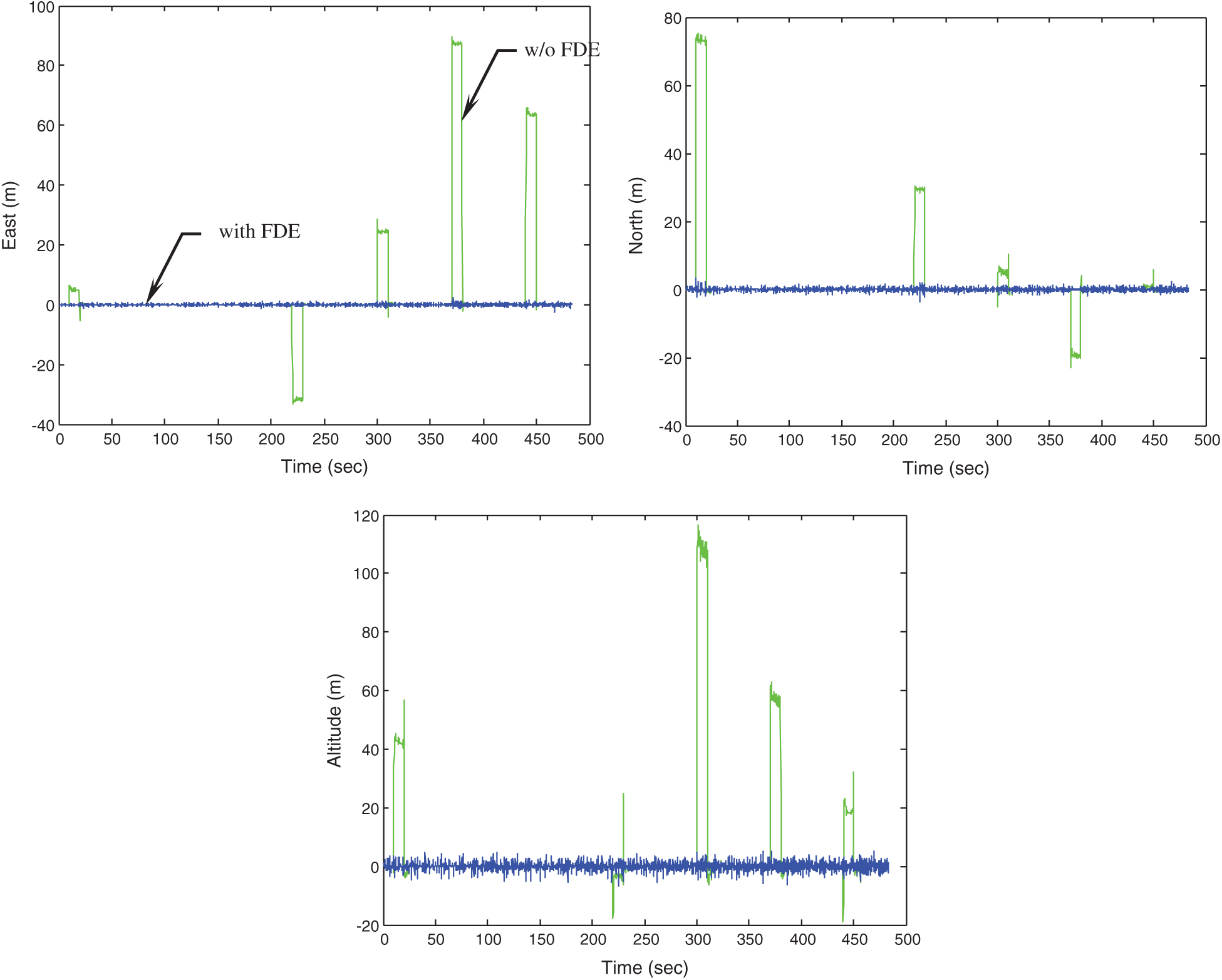
Figure 12: Positioning accuracy for the navigation algorithm with and without FDE mechanism

6  Conclusions

The integrity monitoring algorithms in this work is implemented dealing with the reliability enhancement of the tracking loops. Navigation system integrity refers to the ability of the system to provide timely warning to users when the system should not be used for navigation. The most significant drawback in the VTL is that the failure of tracking in one channel may affect the entire system and lead to loss of lock on all satellites. The scenarios involved in the numerical experiments cover two aspects. The first aspect deals with performance comparison for VTL- and STL-based architectures for various numbers of visible satellites. The second one deals with reliability enhancement when the RAIM and FDE mechanisms are incorporated into the VTL.

The RAIM and the FDE mechanisms have been incorporated into the vector tracking loop architecture where the RAIM mechanism is used to check the possible fault in the pseudorange and the pseudorange rate, and the FDE mechanism is employed for excluding the wrong satellite signal. When the FDE algorithm is incorporated, the vector tracking loop can prevent the failure of one channel from spreading into the entire tracking loop. The feasibility of the proposed approach has been demonstrated for various scenarios. Performance evaluation for the VTL with FDE has been presented. The reliability enhancement for the vector tracking loop has been demonstrated.

Funding Statement: This work has been partially supported by the Ministry of Science and Technology, Taiwan [Grant numbers MOST 104-2221-E-019-026-MY3 and MOST 109-2221-E-019-010].

Conflicts of Interest: The authors declare that they have no conflicts of interest to report regarding the present study.

References

 1.  E. D. Kaplan and C. J. Hegarty, Understanding GPS: Principles and Applications. Norwood, MA, USA: Artech House, Inc., 2006. [Google Scholar]

 2.  J. A. Farrell and M. Barth, The Global Positioning System and Inertial Navigation. New York, NY, USA: McGraw-Hill, 1999. [Google Scholar]

 3.  B. W. Parkinson, J. J. Spilker, P. Axelrad and P. Enge, Global Positioning System: Theory and Applications. Washington, DC, USA: American Institute of Aeronautics and Astronautics, Inc., 1996. [Google Scholar]

 4.  J. Qi, Q. Song and J. Feng, “A novel edge computing based area navigation scheme,” Computers Materials & Continua, vol. 65, no. 3, pp. 2385–2396, 2020. [Google Scholar]

 5.  T. Zhou, B. Lian, S. Yang, Y. Zhang and Y. Liu, “Improved GNSS cooperation positioning algorithm for indoor localization,” Computers Materials & Continua, vol. 56, no. 2, pp. 225–245, 2018. [Google Scholar]

 6.  T. Pany and B. Eissfeller, “Use of a vector delay lock loop receiver for GNSS signal power analysis in bad signal conditions,” in Proc. 2006 IEEE/ION Position, Location, and Navigation Symposium (PLANSCoronado, CA, USA, pp. 893–903, 2006. [Google Scholar]

 7.  M. Lashley, D. M. Bevly and J. Y. Hung, “Performance analysis of vector tracking algorithms for weak GPS signals in high dynamics,” IEEE Journal of Selected Topics in Signal Processing, vol. 3, no. 4, pp. 661–673, 2009. [Google Scholar]

 8.  M. Lashley and D. M. Bevly, “Comparison in the performance of the vector delay/frequency lock loop and equivalent scalar tracking loops in dense foliage and urban canyon,” in Proc. 24th International Technical Meeting of the Institute of Navigation, Portland, OR, USA, pp. 1786–1803, 2011. [Google Scholar]

 9.  Z. Zhu, Z. Cheng, G. Tang, S. Li and F. Huang, “EKF based vector delay lock loop algorithm for GPS signal tracking,” in Proc. 2010 Int. Conf. on Computer Design and Applications, Qinhuangdao, China, 4, pp. 352–356, 2010. [Google Scholar]

10. S. Peng, Y. Morton and R. Di, “A multiple-frequency GPS software receiver design based on a vector tracking loop,” in Proc. 2012 IEEE/ION Position, Location and Navigation Symposium (PLANSMyrtle Beach, SC, USA, pp. 495–505, 2012. [Google Scholar]

11. H. Li and J. Yang, “Analysis and simulation of vector tracking algorithms for weak GPS signal,” in Proc. 2nd Int. Asia Conf. on Informatics in Control, Automation and Robotics, Wuhan, China, pp. 215–218, 2010. [Google Scholar]

12. R. G. Brown, “A baseline GPS RAIM scheme and a note on the equivalence of three RAIM methods,” NAVIGATION: Journal of the Institute of Navigation, vol. 39, no. 3, pp. 301–316, 1992. [Google Scholar]

13. G. Y. Chin, J. Kraemer and R. G. Brown, “GPS RAIM: Screening out bad geometries under worst-case bias conditions,” NAVIGATION: Journal of the Institute of Navigation, vol. 39, no. 4, pp. 407–428, 1992–1993. [Google Scholar]

14. M. Brenner, “Integrated GPS/inertial fault detection availability,” NAVIGATION: Journal of the Institute of Navigation, vol. 43, no. 2, pp. 111–130, 1996. [Google Scholar]

15. J. Diesel and S. Luu, “GPS/IRS AIME: Calculation of thresholds and protection radius using Chi-square methods,” in Proc. ION GPS-95, Palm Springs, CA, USA, pp. 1959–1964, 1995. [Google Scholar]

16. H. Leppäkoski, H. Kuusniemi and J. Takala, “RAIM and complementary Kalman filtering for GNSS reliability enhancement,” in Proc. 2006 IEEE/ION Position, Location, and Navigation Symposium (PLANSCoronado, CA, USA, pp. 948–956, 2006. [Google Scholar]

17. K. Kuusniemi, A. Wieser, G. Lachapelle and J. Takala, “User-level reliability monitoring in urban personal satellite-navigation,” IEEE Transactions on Aerospace and Electronic Systems, vol. 43, no. 4, pp. 1305–1318, 2007. [Google Scholar]

18. A. Gelb, Applied Optimal Estimation. Cambridge, MA, USA: MIT Press, 1974. [Google Scholar]

19. R. G. Brown and P. Y. C. Hwang, Introduction to Random Signals and Applied Kalman Filtering. New York, NY, USA: John Wiley & Sons, 1997. [Google Scholar]

20. GPSoft LLC., Satellite Navigation Toolbox 3.0 User’s Guide. Athens, OH, USA, 2003. [Google Scholar]

This work is licensed under a Creative Commons Attribution 4.0 International License, which permits unrestricted use, distribution, and reproduction in any medium, provided the original work is properly cited.