DOI:10.32604/cmc.2021.016097
| Computers, Materials & Continua DOI:10.32604/cmc.2021.016097 | |
| Article |
Flower Pollination Heuristics for Parameter Estimation of Electromagnetic Plane Waves
1Department of Electronics, University of Peshawar, Peshawar, 25120, Pakistan
2Future Technology Research Center, National Yunlin University of Science and Technology, Douliou, 64002, Taiwan
3Department of Electrical Engineering, International Islamic University, Islamabad, 44000, Pakistan
4Department of Electrical Engineering, COMSATS University Islamabad, Islamabad, 44000, Pakistan
5Department of Computer Science and Information, College of Science in Zulfi, Majmaah University, Al-Majmaah, 11952, Saudi Arabia
*Corresponding Author: Muhammad Asif Zahoor Raja. Email: rajamaz@yuntech.edu.tw
Received: 22 December 2020; Accepted: 02 February 2021
Abstract: For the last few decades, the parameter estimation of electromagnetic plane waves i.e., far field sources, impinging on antenna array geometries has attracted a lot of researchers due to their use in radar, sonar and under water acoustic environments. In this work, nature inspired heuristics based on the flower pollination algorithm (FPA) is designed for the estimation problem of amplitude and direction of arrival of far field sources impinging on uniform linear array (ULA). Using the approximation in mean squared error sense, a fitness function of the problem is developed and the strength of the FPA is utilized for optimization of the cost function representing scenarios for various number of sources non-coherent located in the far field. The worth of the proposed FPA based nature inspired computing heuristic is established through assessment studies on fitness, histograms, cumulative distribution function and box plots analysis. The other worthy perks of the proposed scheme include simplicity of concept, ease in the implementation, extendibility and wide range of applicability to solve complex optimization problems. These salient features make the proposed approach as an attractive alternative to be exploited for solving different parameter estimation problems arising in nonlinear systems, power signal modelling, image processing and fault diagnosis.
Keywords: Direction of arrival; flower pollination algorithm; plane waves; parameter estimation
Parameter estimation specially direction of arrival (DOA) estimation of plane waves plays a vital role in the areas of wireless communication, earthquake, medicine, tracking, navigation, and radio astronomy [1–4]. In this regard, incorporation of beamforming being adaptive in smart antennas systems gives opportunities to reduce the interferences effects and without using the higher frequency bandwidths, data is transmitted at higher rates. This essential requirement stimulates for the development of algorithms being efficient to estimate DOA. This helps in the determination of complex weights required in beamsteering for preferred direction. Traditional techniques used for estimation of DOA employed the method of periodogram which was based on Fourier transformation. A few of them are conventional beamforming (CBF), Minimum Variance Distortion less Response (MVDR) and dual beamformer. Bartlett, Capon and Lacoss are their developers [5–7]. The problem with the traditional method was low resolution and further, noise due to Rayleigh limit affected it badly.
To overcome these problems adaptive algorithms were used and methods of maximum likelihood were developed. Stochastic maximum likelihood and deterministic maximum likelihood i.e., SML and DML methods were a few to mention [8,9]. Technique of spatial-temporal processing further improved the accuracy of DML [10]. These methods were having better resolution due to using data model of the received signals completely. Also, these were robust and efficient. But their computational cost is too high due to the multidimensional search and are therefore used occasionally [10,11]. The spectrum-based methods developed in 1980s, were Multiple Signal Classification (MUSIC), Estimation of Signal Parameters via Rotational Invariance Technique (ESPRIT) [12,13]. But the problem with these methods was their computational cost that kept increasing with the increase in the number of array element as they required snapshots at least double in number of the total number of elements in the array. Also, in case of correlated signals, their performance becomes poor. Unitary-ESPRIT method was introduced that was based on unitary transformation and its purpose was to reduce computing cost of ESPRIT method. Conversion of complex covariance matrix into real one reduced its complexity of computation [14]. To rectify the problems in covariance based methods, Direct Data Domain Methods (DDDMs) were developed in mid-nineties. They were based on Matrix Pencil Method (PM) [15]. They were efficient and they required one snapshot in case of DOA to be estimated in real time dynamic conditions.
Techniques, being metaheuristic, have been exploited for the determination of DOA unlike adaptive techniques namely Least Mean Square, MUSIC, ESPRIT and Recursive Least Square etc. due to their effective strength in optimization [16–19]. To address numerous non-linear problems of constrained optimization in different areas such as optimal energy management, combustion theory fuel ignition model, Magneto-hydrodynamics problems, electromagnetic theory, nano-technology and fractional order systems of non-linear nature [20–25], techniques of evolution and swarm intelligence have been applied to them recently.
In this paper, an effective optimization mechanism of flower pollination algorithm (FPA) is employed as a newly introduced algorithm for the parameter estimation of electromagnetic waves of the far field. FPA mimics the process of pollination in flowering plants. FPA is proposed by Yang [26] and is recently employed in several fields. FPA has impressive nature. Due to this, it has attracted many researchers’ attention in several fields of optimization. Swarm-based optimization technique is used in the FPA with few parameters. The employment of the FPA in various optimization problems has shown a robust performance. Further, FPA being simple optimization method is a flexible, adaptable, and scalable algorithm. FPA gives very beneficial results in solving various optimization problems as compared with other metaheuristic algorithms. These problems are from different areas such as signal and image processing, clustering and classification, electrical systems, wireless networks, computer gaming, travelling salesman problem and others many more [27–48]. In the present work collective estimation of DOA as well as amplitudes of plane wave (electromagnetic) falling on ULA is considered. To minimize error between desired and actual responses, mean squared error (MSE) is used as a fitness criterion. A single snapshot is required by this fitness function and works well, particularly in the existence of local optima. For substantial statistical analysis of FPA, Monte Carlo simulations (in a large number) are done using MATLAB. For this analysis two, three, and four sources are considered and are investigated for fitness, robustness, MSE, and complexity (computational). Main properties of the proposed mechanism are as follows:
• Exploitation of pollination based optimization technique FPA for the novel study of DOA estimation
• Augmented power of FPA is built for the parameter estimation (effectively) of plane waves of sources.
• The design mechanism is validated for different scenarios of far field sources.
• The accuracy, robustness, and reliability of the algorithm are proven via results of the statistics in terms of parameters fitness.
• Ease of implementation, simple in concept, extendibility, handling complex models and wide range of applicability are further advantages of the scheme.
The paper is arranged as follows: In Section 2, plane waves incident on a ULA is given as general data model for parameter estimation, while details about proposed scheme that has foundation on FPA are given in Section 3. Section 4 provides results and discussion on the results. The last section presents the conclusion and future work.
2 General System Model for Parameters Amplitude and DOA Estimation
For model development, consider narrow band sources of EM plane waves P in number. The plane waves are falling on ULA. The ULA has “N” elements. The inter-element spacing is “d” which is uniform between any two consecutive elements. It is portrayed in Fig. 1. For
for
In Eq. (2), the value of
Here
S is the symbol used here for the steering matrix. It has got steering vectors of P sources. AWGN introduced in each antenna element is symbolized here as
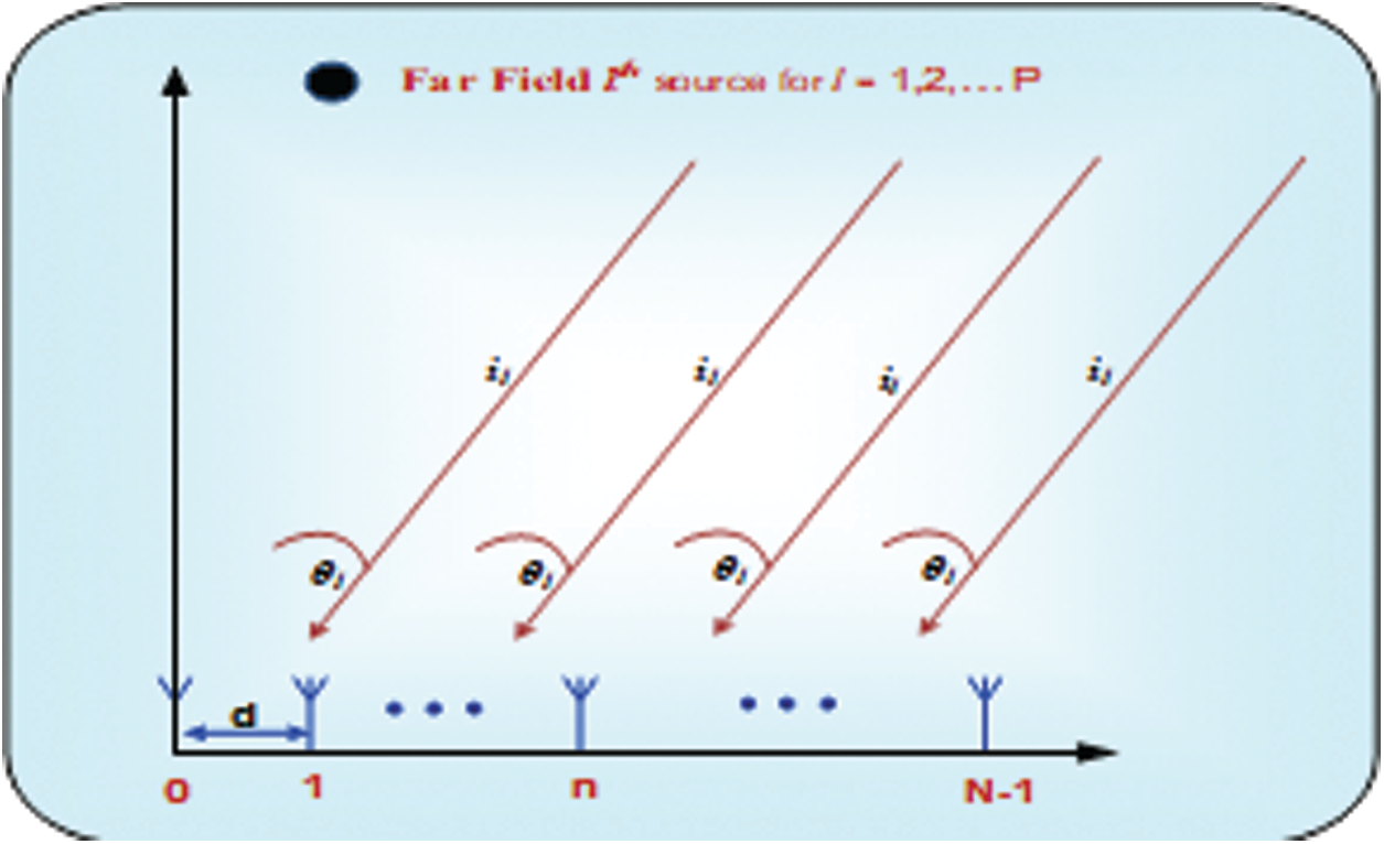
Figure 1: Plane waves falling on ULA antenna
A new meta heuristic technique called FPA was originally proposed by Yang [26] in 2012. This algorithm uses the concept of pollination in plants. Pollination is prerequisite of the fertilization in plant species. In this process pollens migrate, meet the pollens of another flower or other plants. The flower may be of the same plant. Likewise, the other plants may be of same species. This results in fruitful fertilization. In biotic pollination, pollinators (insects/birds etc.) are carriers of the pollens from one flower to another. The same are transferred via wind or simple diffusion in abiotic pollination. Most of the part is played by the biotic pollination in nature. Flower constancy for pollination is another responsible factor. In this, pollinators limit themselves with plants of particular type. [49]. The mathematical expression for FPA is written as [49]:
In Eq. (5),
In this work, FPA is developed for parameter estimation of electromagnetic plane waves. The flow chart of FPA is portrayed in Fig. 2. While, the pseudo-code is given as follows:
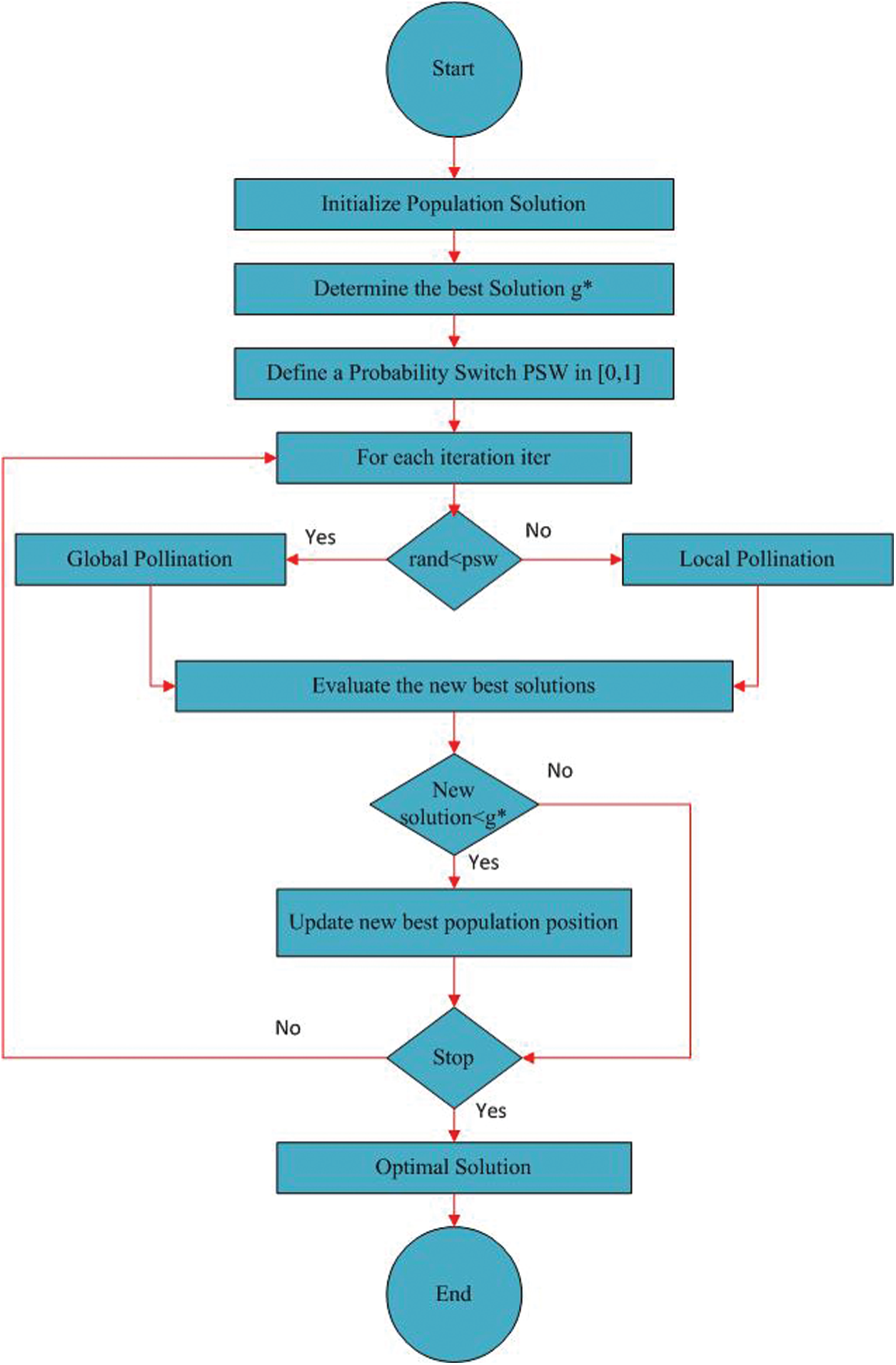
Figure 2: Flow chart of FPA
Step 1 Population Initialization
“M” individuals are generated randomly with entries equal to decision variable of optimization problem, i.e., DOA estimation of plane waves. The Jth individual representation of FPA is mathematically given as:
For the current optimization problem, the constraints associated with are:
Amplitude bounds (lower and upper) are symbolized here as lb and ub respectively, and
Step 2 Computation of Fitness
The fitness function is expressed in terms of mean squared error. For noiseless environment it is given as:
Fitness is computed for each individual of population F using Eq. (7) and are ranked accordingly.
Step 3 Determine g*, the initial best solution
Step 4 Defines a probability switch
Step 5 Compute fitness value of all n members/solution/flowers.
Step 6 if
Step 7 Draw a step vector L (d-dimensional) obeying Levy Distribution
Step 8 Carry out global pollination via
Else
Step 9 Draw a uniform distribution
Step 10 Randomly choose j and k among all solutions
Step 11 Do local pollination via
Step 12 Evaluate the new best solution
Step 13 If the new
Step 14 xt = xt+1
Step 15 Find the current best solution
Step 16 For global best solution, store the parameters, and its fitness for each run.
Step 17 For reliability, Steps 1–16 are repeated for sufficiently huge runs to have a huge set of data.
Step 18 For FPA performance evaluation, the fitness as in Eq. (7) and norm of the absolute error (NAE), also called the Euclidean length, as defined below are used:
where N is index of element in vector v.
In this section, work is presented in terms of simulations for three scenarios. In each scenario we have two sources model (2SM), three sources model (3SM) and four sources model (4SM). The EM plane wave sources are P where
The scheme designed (based on FPA) is utilized for parameter estimation. It is employed for both situations (noisy as well as noiseless) as given in the section of methodology. For each scenario, five cases are worked out as: Case 1: 2 SM with no noise and given noise is added for rest of the four cases namely Case 2: 2 SM having 65 dB, Case 3: 2 SM having 55 dB, Case 4: 2 SM having 45dB and Case 5: 2 SM having 35 dB. The results are obtained for 100 independent runs of the FPA. Objective function for any of the scenario is formulated as:
Eq. (9) denotes fitness function. In this
For this data, the algorithm was run 100 times independently. The best estimated parameters are given in Tabs. 1–3 for all the three scenarios. Analysis of the data was done in terms of fitness, histogram, CDF and Box Plots for two different types. In type1 analysis, different number of sources were taken, and same level of noise was added to them. Five such cases were examined namely no noise, 35 dB noise, 45 dB noise, 55 dB noise and 65 dB noise. In the 2nd type, same number of sources were taken, and different noise was added to it. Again, same five levels of noise were added in steps. Two of the graphs of type 1 analysis with no noise and with 65 dB noise are provided for fitness, histogram, CDF and Box Plot respectively in Figs. 3–6. The graphs of the 2nd type analysis are shown in Figs. 7–10. Fig. 3a shows that the best fitness of two sources is about 10−29 in 85 runs. Three sources reach to a fitness of about 10−28 in 96 runs. Likewise, four sources have about 10−7 fitness in 100 runs. Remaining graphs of the 1st case can also be shown. Likewise, Fig. 3b shows that even though 65 dB noise has been added but still the same two sources get a fitness of about 10−31 in about 88 runs. The same three sources get a fitness of about 10−30 in about 97 runs and the same four sources get a fitness of about 10−8 in 100 runs.
Table 1: Outcomes of FPA for scenario 1 of two far field sources

Table 2: Outcomes of FPA for scenario 2 of three far field sources
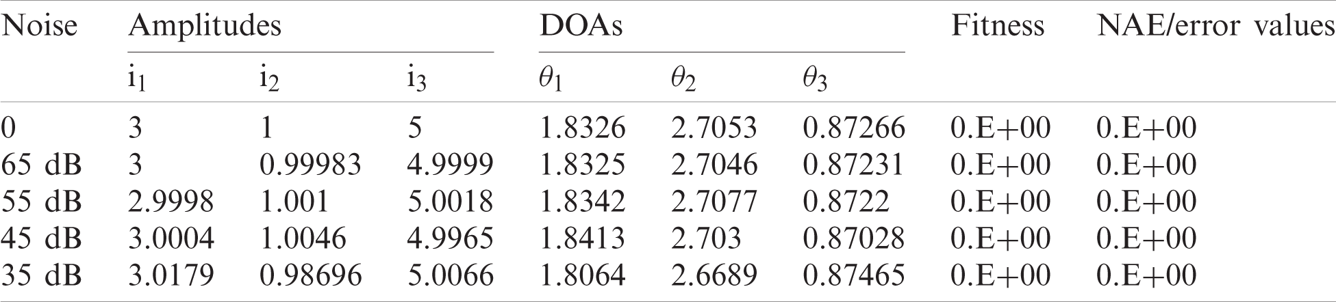
Table 3: Outcomes of FPA for scenario 3 of four far field sources
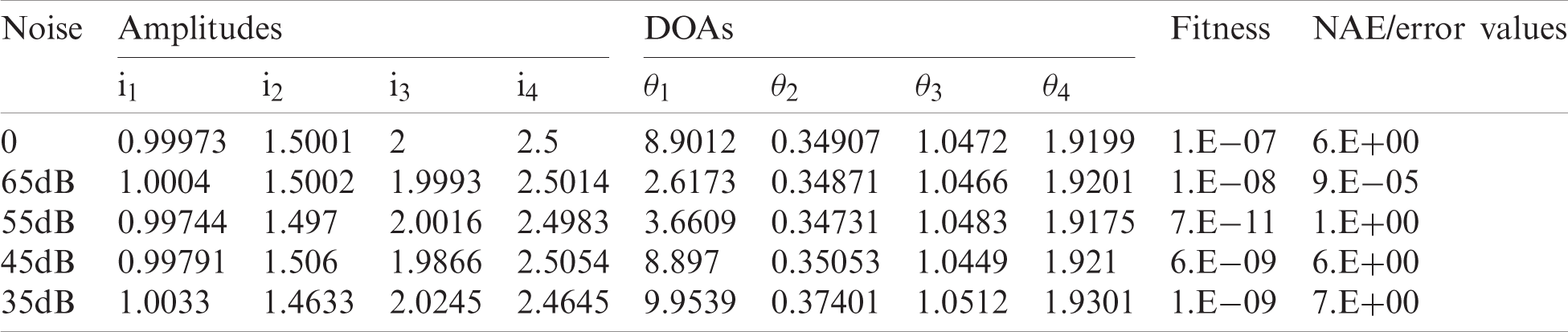
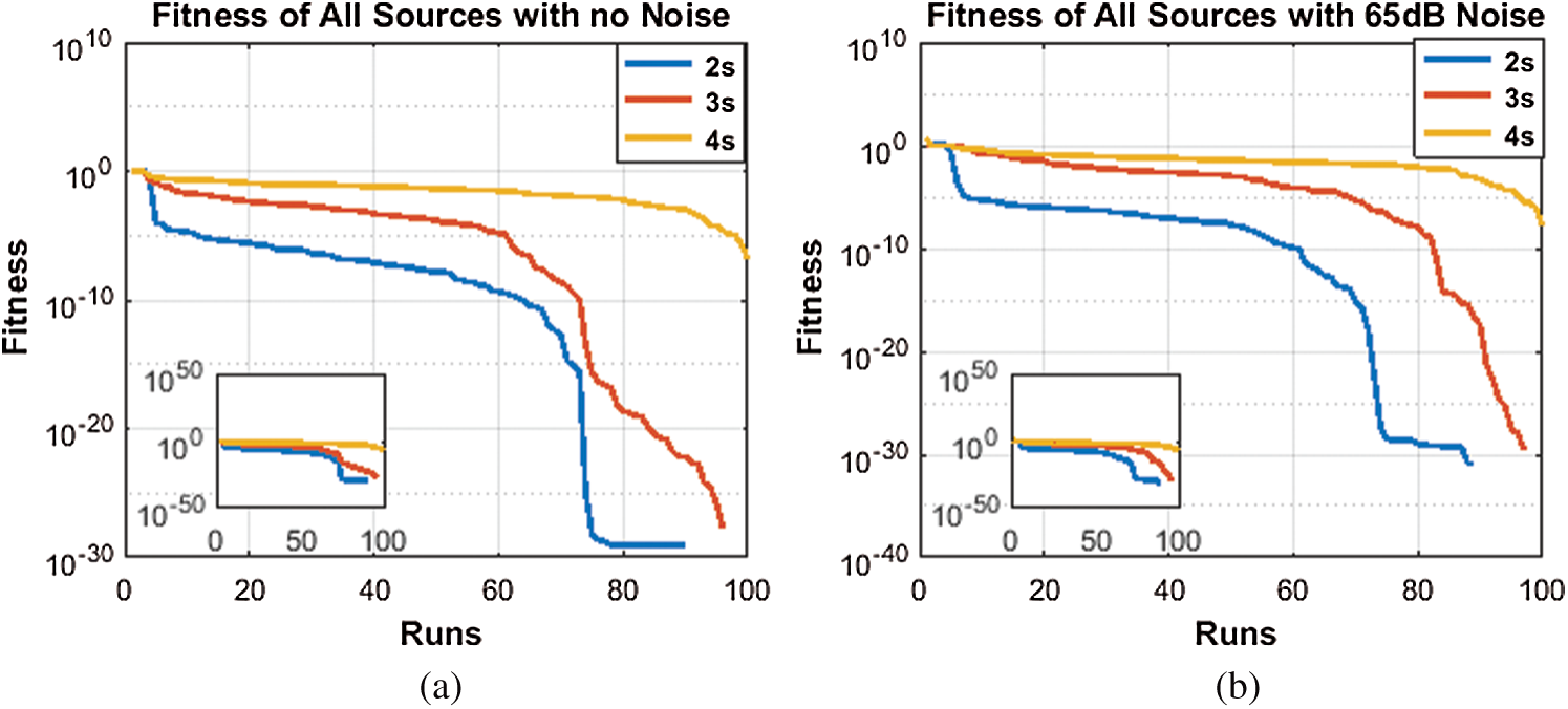
Figure 3: Fitness with and without noise. (a) No noise case, (b) 65 dB noise case

Figure 4: Histogram with and without noise. (a)No noise case, (b) 65 dB noise case
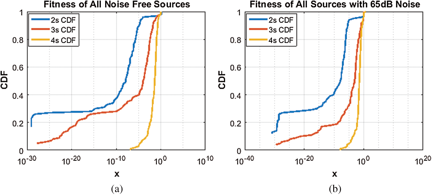
Figure 5: CDF with and without noise. (a)No noise case, (b) 65 dB noise case
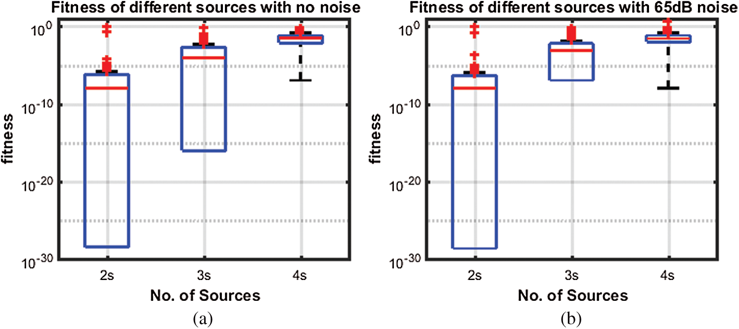
Figure 6: Box Plots with and without noise. (a)No noise, case (b)65 dB noise case
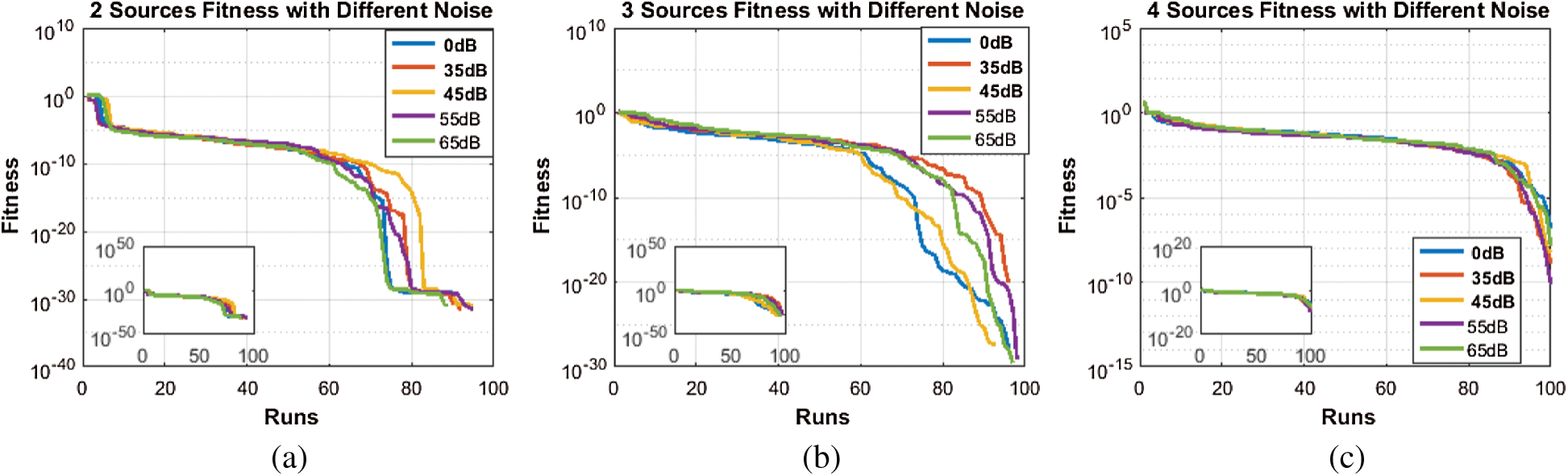
Figure 7: Fitness of same source with different noise. (a) 2 sources (b) 3 sources (c) 4 sources

Figure 8: Histogram of same source with different noise. (a) 2 sources (b) 3 sources (c) 4 sources
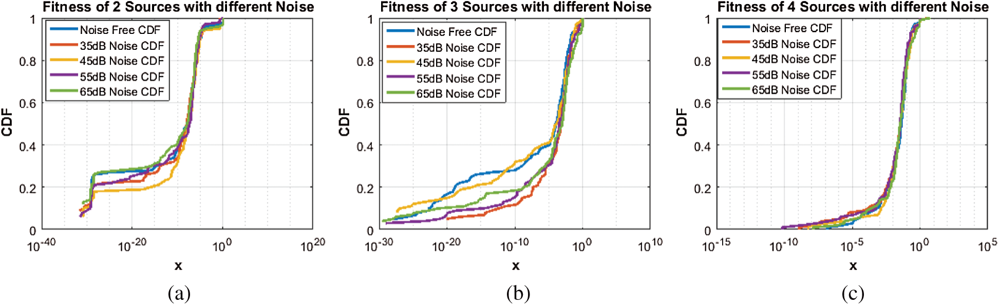
Figure 9: CDF of same source with different noise. (a) 2 sources (b) 3 sources (c) 4 sources
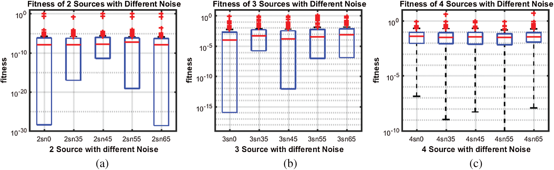
Figure 10: Box plot of same source with different noise. (a) 2 sources (b) 3 sources (c) 4 sources
Fig. 4 shows the histogram analysis of the same two cases namely noise free and with 65 dB noise. Fig. 4a shows that about 16 runs give a fitness in the range of 10−30 to 10−25 for two sources, and about 2 runs give the same fitness for three sources while the same two runs give a fitness in the range 10−20 to 10−15 for four sources. Fig. 4b shows that 2 runs give a fitness in the range of 10−35 to 10−30 for two sources, 4 runs give a fitness in the range of 10−30 to 10−25 for three sources, and about 2 runs give a fitness of 10−6 to 10−5 for four sources in the presence of 65 dB noise respectively. Fig. 5 shows the CDF analysis of the same two cases namely noise free and with 65 dB noise. Fig. 5a shows that about 17% of the runs give a fitness of 10−29 for two sources, about 5% of runs give a fitness of more than 10−27 for three sources and about a fraction of one run gives a fitness of about 10−7 for four sources. Fig. 5b shows a fitness of about 10−31 for about 12% of the runs for two sources, a fitness of more than 10−29 for 4% of runs for three sources, and a fitness of about 10−8 for about a fraction of 1% runs for four sources in presence of 65dB noise. Fig. 6 shows the box plot analysis for the same two cases namely noise free and with 65 dB noise. Fig. 6a shows that worst fitness is about 10−6 for two sources, more than 10−2 for three sources and more than 10−1 for four sources. Likewise, the best fitness is more than 10−28 for two sources, about 10−16 for three sources and about 10−7 for four sources. 75% of fitness is about 10−6 for two sources, less than 10−3 for three sources and about 10−1 for four sources. Exactly half of the fitness is about 10−8 for two sources, 10−4 for three sources and less than 10−1 for four sources. Fig. 6b shows that worst fitness is less than 10−4 for two sources, less than 10−2 for three sources, and less than 10−1 for four sources. Likewise, the best fitness is more than 10−28 for two sources, about 10−7 for three sources, and 10−8 for four sources. 75% of the fitness is about 10−6 for two sources, 10−2 for three sources and 10−1 for four sources. Exactly half of the fitness is about 10−8 for two sources, 10−3 for three sources, and less than 10−1 for four sources in the presence of 65 dB noise.
Likewise, all Figs. 7–10 results show that even in low SNR situation, the proposed algorithm performed well. With low estimation accuracy, particularly in case of two and three sources, it has produced fair enough results. However, its performance is degraded in case of four impinging sources. The reason is clear that as number of sources increases, problem of identification becomes harder.
An innovative application of flower pollination heuristic is introduced for reliable parameter estimation of electromagnetic plane waves impinging on antenna array geometries. The accuracy, stability and robustness of the proposed flower pollination heuristic is verified from actual value of system parameter for single and multiple autonomous runs. The worth of the proposed FPA is further established through statistical assessments based on fitness, histograms, cumulative distribution function and box plots analysis for two, three and four source model of DOA parameter estimation in noisy and noiseless environments.
In future, one may exploit the proposed methodology for different optimization problems including power signal estimation [50], Hammerstein nonlinear system identification [51–53], fault diagnosis [54], travelling salesman problem [55], second order boundary value problems [56] and image processing [57].
Funding Statement: The authors would like to thank the Deanship of Scientific Research at Majmaah University for supporting this work under Project Number No. R-2021-27.
Conflicts of Interest: All the authors of the manuscript declared that there are no potential conflicts of interest.
1. T. E. Tuncer and B. Friedlander, Classical and Modern Direction of Arrival Estimation. Burlington, MA: Elsevier Inc., 2009. [Google Scholar]
2. C. L. Meng, S. W. Chen and A. C. Chang, “Direction-of-arrival estimation based on particle swarm optimization searching approaches for CDMA signals,” Wireless Personal Communications, vol. 81, no. 1, pp. 343–357, 2015. [Google Scholar]
3. R. Cao, C. Wang and X. Zhang, “Two-dimensional direction of arrival estimation using generalized ESPRIT algorithm with non-uniform L-shaped array,” Wireless Personal Communications, vol. 84, no. 1, pp. 321–339, 2015. [Google Scholar]
4. Z. Chen, G. K. Gokeda and Y. Yu, Introduction to Direction-of-Arrival Estimation. Norwood: Artech House, 2010. [Google Scholar]
5. M. S. Bartlett, “Smoothing periodograms from time series with continuous spectra,” Nature, vol. 161, no. 4096, pp. 686–687, 1948. [Google Scholar]
6. J. Capon, “High resolution frequency-wavenumber spectrum analysis,” Proceedings of the IEEE, vol. 57, no. 8, pp. 1408–1418, 1969. [Google Scholar]
7. R. T. Lacoss, “Data adaptive spectral analysis methods,” Geophysics, vol. 36, no. 4, pp. 661–675, 1971. [Google Scholar]
8. P. Stoica and K. C. Sharman, “Maximum likelihood methods for direction-of-arrival estimation,” IEEE Transactions on Acoustics, Speech, and Signal Processing, vol. 38, no. 7, pp. 1132–1143, 1990. [Google Scholar]
9. M. I. Miller and D. R. Fuhrmann, “Maximum-likelihood narrow-band direction finding and the EM algorithm,” IEEE Transactions on Acoustics, Speech, and Signal Processing, vol. 38, no. 9, pp. 1560–1577, 1990. [Google Scholar]
10. L. C. Godara, “Application of antenna arrays to mobile communications. II. Beam-forming and direction-of-arrival considerations,” Proc. of the IEEE, vol. 85, no. 8, pp. 1195–1245, 1997. [Google Scholar]
11. Z. Ariela and B. Friedlander, “Direction of arrival estimation using parametric signal models,” IEEE Transactions on Signal Processing, vol. 44, no. 2, pp. 339–350, 1996. [Google Scholar]
12. F. Richard, “Analysis of min-norm and MUSIC with arbitrary array geometry,” IEEE Transactions on Aerospace and Electronic Systems, vol. 26, no. 6, pp. 976–985, 1990. [Google Scholar]
13. M. Haardt and M. E. Ali-Hackl, “Unitary ESPRIT: How to exploit additional information inherent in the rotational invariance structure,” in ICASSP Proc., Adelaide, Australia, pp. 229–232, 1994. [Google Scholar]
14. H. Krim and J. G. Proakis, “Smoothed eigenspace-based parameter estimation,” Automatica, vol. 30, no. 1, pp. 27–38, 1994. [Google Scholar]
15. Y. Hua and T. K. Sarkar, “Matrix pencil method for estimating parameters of exponentially damped-undamped sinusoids in noise,” IEEE Transactions on Acoustics, Speech, and Signal Processing, vol. 38, no. 5, pp. 814–824, 1990. [Google Scholar]
16. M. Li and Y. Lu, “A refined genetic algorithm for accurate and reliable DOA estimation with a sensor array,” Wireless Personal Communications, vol. 43, no. 2, pp. 533–547, 2007. [Google Scholar]
17. L. Boccato, R. Krummenauer, R. Attux and A. Lopes, “Application of natural computing algorithms to maximum likelihood estimation of direction of arrival,” Signal Processing, vol. 92, no. 5, pp. 1338–1352, 2012. [Google Scholar]
18. L. Boccato, R. Krummenauer, R. Attux and A. Lopes, “Improving the efficiency of natural computing algorithms in DOA estimation using a noise filtering approach,” Circuits, Systems, and Signal Processing, vol. 32, no. 4, pp. 1991–2001, 2013. [Google Scholar]
19. Z. Zhang, J. Lin and Y. Shi, “Application of artificial bee colony algorithm to maximum likelihood DOA estimation,” Journal of Bionic Engineering, vol. 10, no. 1, pp. 100–109, 2013. [Google Scholar]
20. J. A. Khan, M. A. Z. Raja, M. M. Rashidi, M. I. Syam and A. M. Wazwaz, “Nature-inspired computing approach for solving non-linear singular Emden–Fowler problem arising in electromagnetic theory,” Connection Sciences, vol. 27, no. 4, pp. 377–396, 2015. [Google Scholar]
21. M. A. Z. Raja, “Solution of the one-dimensional Bratu equation arising in the fuel ignition model using ANN optimised with PSO and SQP,” Connection Science, vol. 26, no. 3, pp. 195–214, 2014. [Google Scholar]
22. M. A. Z. Raja and R. Samar, “Numerical treatment for nonlinear MHD Jeffery-Hamel problem using neural networks optimized with interior point algorithm,” Neurocomputing, vol. 124, no. 29, pp. 178–193, 2014. [Google Scholar]
23. H. Xia, H. Chen, Z. Yang, F. Lin and B. Wang, “Optimal energy management, location and size for stationary energy storage system in a metro line based on genetic algorithm,” Energies, vol. 8, no. 10, pp. 11618–11640, 2015. [Google Scholar]
24. M. A. Z. Raja, U. Farooq, N. I. Chaudhary and A. M. Wazwaz, “Stochastic numerical solver for nanofluidic problems containing multi-walled carbon nanotubes,” Applied Soft Computing, vol. 38, no. 6348, pp. 561–586, 2015. [Google Scholar]
25. M. A. Z. Raja, M. A. Manzar and R. Samar, “An efficient computational intelligence approach for solving fractional order Riccati equations using ANN and SQP,” Applied Mathematical Modeling, vol. 39, no. 10,11, pp. 3075–3093, 2015. [Google Scholar]
26. X. S. Yang, “Flower pollination algorithm for global optimization,” in UCNC Lecture Notes in Computer Science, vol. 7445. Berlin, Heidelberg: Springer, pp. 240–249, 2012. https://doi.org/10.1007/978-3-642-32894-7_27. [Google Scholar]
27. A. Abdelaziz, E. Ali and S. A. Elazim, “Combined economic and emission dispatch solution using flower pollination algorithm,” International Journal of Electrical Power & Energy Systems, vol. 80, no. 4, pp. 264–274, 2016. [Google Scholar]
28. U. Singh and R. Salgotra, “Synthesis of linear antenna array using flower pollination Algorithm,” Neural Computing and Applications, vol. 29, no. 2, pp. 435–445, 2018. [Google Scholar]
29. A. Abdelaziz, E. Ali and S. A. Elazim, “Implementation of flower pollination algorithm for solving economic load dispatch and combined economic emission dispatch problems in power systems,” Energy, vol. 101, no. 1, pp. 506–518, 2016. [Google Scholar]
30. W. Zhang, Z. Qu, K. Zhang, W. Mao, Y. Ma et al., “A combined model based on CEEMDAN and modified flower pollination algorithm for wind speed forecasting,” Energy Conversion and Management, vol. 136, no. 995, pp. 439–451, 2017. [Google Scholar]
31. T. T. Nguyen, J. S. Pan and T. K. Dao, “An improved flower pollination algorithm for optimizing layouts of nodes in wireless sensor network,” IEEE Access, vol. 7, pp. 75985–75998, 2019. [Google Scholar]
32. D. Rodrigues, G. F. Silva, J. P. Papa, A. N. Marana and X.-S. Yang, “Eeg-based person identification through binary flower pollination algorithm,” Expert Systems with Applications, vol. 62, no. 4, pp. 81–90, 2016. [Google Scholar]
33. E. Emary, H. M. Zawbaa, A. E. Hassanien and B. Parv, “Multi-objective retinal vessel localization using flower pollination search algorithm with pattern search,” Advances in Data Analysis and Classification, vol. 11, no. 3, pp. 611–627, 2017. [Google Scholar]
34. S. Ouadfel and A. Taleb-Ahmed, “Social spiders optimization and flower pollination algorithm for multilevel image thresholding: A performance study,” Expert Systems with Applications, vol. 55, no. 2, pp. 566–584, 2016. [Google Scholar]
35. M. Sharawi, E. Emary, I. A. Saroit and H. El-Mahdy, “Flower pollination optimization algorithm for wireless sensor network lifetime global optimization,” International Journal of Soft Computing and Engineering, vol. 4, no. 3, pp. 54–59, 2014. [Google Scholar]
36. T. Shankar, T. James, R. Mageshvaran and A. Rajesh, “Lifetime improvement in wsn using flower pollination meta heuristic algorithm based localization approach,” Indian Journal of Science and Technology, vol. 9, no. 37, pp. 1–10, 2016. [Google Scholar]
37. T. Adithiyaa, D. Chandramohan and T. Sathish, “Flower Pollination Algorithm for the optimization of stair casting parameter for the preparation of AMC,” Materials Today: Proc., vol. 21, no. 6, pp. 882–886, 2020. [Google Scholar]
38. H. Chiroma, A. Khan, A. I. Abubakar, Y. Saadi, M. F. Hamza et al., “A new approach for forecasting opec petroleum consumption based on neural network train by using flower pollination algorithm,” Applied Soft Computing, vol. 48, no. 12, pp. 50–58, 2016. [Google Scholar]
39. P. Agarwal and S. Mehta, “Enhanced flower pollination algorithm on data clustering,” International Journal of Computers and Applications, vol. 38, no. 2, 3, pp. 144–155, 2016. [Google Scholar]
40. E. Nabil, “A modified flower pollination algorithm for global optimization,” Expert Systems with Applications, vol. 57, pp. 192–203, 2016. [Google Scholar]
41. K. Priya and N. Rajasekar, “Application of flower pollination algorithm for enhanced proton exchange membrane fuel cell modelling,” International Journal of Hydrogen Energy, vol. 44, no. 33, pp. 18438–18449, 2019. [Google Scholar]
42. K. Wang, X. Li and L. Gao, “A multi-objective discrete flower pollination algorithm for stochastic two-sided partial disassembly line balancing problem,” Computers & Industrial Engineering, vol. 130, no. 6, pp. 634–649, 2019. [Google Scholar]
43. Y. Zhou, R. Wang and Q. Luo, “Elite opposition-based flower pollination algorithm,” Neurocomputing, vol. 188, no. 3, pp. 294–310, 2016. [Google Scholar]
44. L. Shen, C. Fan and X. Huang, “Multi-level image thresholding using modified flower pollination algorithm,” IEEE Access, vol. 6, pp. 30508–30519, 2018. [Google Scholar]
45. M. Abdel-Basset and L. A. Shawky, “Flower pollination algorithm: A comprehensive review,” Artificial Intelligence Review, vol. 52, no. 4, pp. 2533–2557, 2019. [Google Scholar]
46. S. Xu and Y. Wang, “Parameter estimation of photovoltaic modules using a hybrid flower pollination algorithm,” Energy Conversion and Management, vol. 144, pp. 53–68, 2017. [Google Scholar]
47. Z. A. A. Alyasseri, A. T. Khader, M. A. Al-Betar, M. A. Awadallah and X. S. Yang, “Variants of the flower pollination algorithm: A review,” Dimensions, vol. 744, pp. 91–118, 2018. [Google Scholar]
48. F. Zaman, I. M. Qureshi, A. Naveed and Z. U. Khan, “Joint estimation of amplitude, direction of arrival and range of near field sources using memetic computing,” Progress in Electromagnetics Research C, vol. 31, pp. 199–213, 2012. [Google Scholar]
49. X. S. Yang, M. Karamanoglu and X. He, “Flower pollination algorithm: a novel approach for multiobjective optimization,” Engineering Optimization, vol. 46, no. 9, pp. 1222–1237, 2014. [Google Scholar]
50. N. I. Chaudhary, R. Latif, M. A. Z. Raja and J. A. T. Machado, “An innovative fractional order LMS algorithm for power signal parameter estimation,” Applied Mathematical Modelling, vol. 83, no. 6, pp. 703–718, 2020. [Google Scholar]
51. N. I. Chaudhary, M. Ahmed, N. Dedovic and M. A. Z. Raja, “Momentum least mean square paradigm for the measurement of nonlinear CARAR system parameters,” Journal of Computational and Nonlinear Dynamics, vol. 15, no. 3, pp. 31004, 2020. [Google Scholar]
52. N. I. Chaudhary, S. Zubair, M. S. Aslam, M. A. Z. Raja and J. A. T. Machado, “Design of momentum fractional LMS for Hammerstein nonlinear system identification with application to electrically stimulated muscle model,” European Physical Journal Plus, vol. 134, no. 8, pp. 407, 2019. [Google Scholar]
53. N. I. Chaudhary, M. S. Aslam, D. Baleanu and M. A. Z. Raja, “Design of sign fractional optimization paradigms for parameter estimation of nonlinear Hammerstein systems,” Neural Computing and Applications, vol. 32, no. 12, pp. 8381–8399, 2020. [Google Scholar]
54. K. Zhu, S. Ying, N. Zhang, R. Wang, Y. Wu et al., “A performance fault diagnosis method for SaaS software based on GBDT algorithm,” Computers, Materials and Continua, vol. 62, no. 3, pp. 1161–1185, 2020. [Google Scholar]
55. Y. Ruan, S. Marsh, X. Xue, Z. Liu and J. Wang, “The quantum approximate algorithm for solving traveling salesman problem,” Computers, Materials and Continua, vol. 63, no. 3, pp. 1237–1247, 2020. [Google Scholar]
56. C. Anitescu, E. Atroshchenko, N. Alajlan and T. Rabczuk, “Artificial neural network methods for the solution of second order boundary value problems,” Computers, Materials and Continua, vol. 59, no. 1, pp. 345–359, 2019. [Google Scholar]
57. F. Li, C. Ou, Y. Gui and L. Xiang, “Instant edit propagation on images based on bilateral grid,” Computers, Materials and Continua, vol. 61, no. 2, pp. 643–656, 2019. [Google Scholar]
 | This work is licensed under a Creative Commons Attribution 4.0 International License, which permits unrestricted use, distribution, and reproduction in any medium, provided the original work is properly cited. |