DOI:10.32604/cmc.2021.015916
| Computers, Materials & Continua DOI:10.32604/cmc.2021.015916 | |
| Article |
Gastric Tract Disease Recognition Using Optimized Deep Learning Features
1Department of Computer Science, HITEC University, Taxila, 47040, Pakistan
2Department of Computer Engineering, College of Computer and Information Sciences, King Saud University, Riyadh, 11543, Saudi Arabia
3Department of Computer Science and Engineering, Soonchunhyang University, Asan, Korea
4Department of Mathematics and Computer Science, Faculty of Science, Beirut Arab University, Beirut, Lebanon
*Corresponding Author: Yunyoung Nam. Email: ynam@sch.ac.kr
Received: 14 December 2020; Accepted: 13 February 2021
Abstract: Artificial intelligence aids for healthcare have received a great deal of attention. Approximately one million patients with gastrointestinal diseases have been diagnosed via wireless capsule endoscopy (WCE). Early diagnosis facilitates appropriate treatment and saves lives. Deep learning-based techniques have been used to identify gastrointestinal ulcers, bleeding sites, and polyps. However, small lesions may be misclassified. We developed a deep learning-based best-feature method to classify various stomach diseases evident in WCE images. Initially, we use hybrid contrast enhancement to distinguish diseased from normal regions. Then, a pretrained model is fine-tuned, and further training is done via transfer learning. Deep features are extracted from the last two layers and fused using a vector length-based approach. We improve the genetic algorithm using a fitness function and kurtosis to select optimal features that are graded by a classifier. We evaluate a database containing 24,000 WCE images of ulcers, bleeding sites, polyps, and healthy tissue. The cubic support vector machine classifier was optimal; the average accuracy was 99%.
Keywords: Stomach cancer; contrast enhancement; deep learning; optimization; features fusion
Stomach (gastric) cancer can develop anywhere in the stomach [1] and is curable if detected and treated early [2], for example, before cancer spreads to lymph nodes [3]. The incidence of stomach cancer varies globally. In 2019, the USA reported 27,510 cases (17,230 males and 10,280 females) with 11,140 fatalities (6,800 males and 4,340 females) [4]. In 2018, 26,240 new cases and 10,800 deaths were reported in the USA (https://www.cancer.org/research/cancer-facts-statistics/all-cancer-facts-figures/cancer-facts-figures-2020.html). In Australia, approximately 2,462 cases were diagnosed in 2019 (1,613 males and 849 females) with 1,287 deaths (780 males and 507 females) (www.canceraustralia.gov.au/affected-cancer/cancer-types/stomach-cancer/statistics). Regular endoscopy and wireless capsule endoscopy (WCE) are used to detect stomach cancer [5,6]. Typically, WCE yields 57,000 frames, and all must be checked [7]. Manual inspection is not easy and must be performed by an expert [8]. Automatic classification of stomach conditions has been attempted [9]. Image preprocessing is followed by feature extraction, fusion, and classification [10], and image contrast is enhanced by contrast stretching [11]. The most commonly used features are color, texture, and shape. Some researchers have fused selected features to enhance diagnostic accuracy [12]. Recent advances in deep learning have greatly improved performance [13].
The principal conventional techniques used to detect stomach cancer are least-squares saliency transformation (LSST), a saliency-based method, contour segmentation, and color transformation [14]. Kundu et al. [15] sought to automate WCE frame evaluation employing LSST followed by probabilistic model-fitting; LSST detected the initially optimal coefficient vectors. A saliency/ best-features method was used by Khan et al. [16] to classify stomach conditions using a neural network; the average accuracy was 93%. Khan et al. [7] employed deep learning to identify stomach diseases. Deep features were extracted from both original WCE images and segmented stomach regions; the latter was important in terms of model training. Alaskar et al. [17] established a fully automated method of disease classification. Pretrained deep models (AlexNet and GoogleNet) were used for feature extraction and a softmax classifier was used for classification. A fusion of data processed by two pretrained models enhanced accuracy. Khan et al. [10] used deep learning to classify stomach disease, employing Mask RCNN for segmentation and fine-tuning of ResNet101; the Grasshopper approach was used for feature optimization. Selected features were classified using a multiclass support vector machine (SVM). Wang et al. [18] presented a deep learning approach featuring superpixel segmentation. Initially, each image was divided into multiple slices and superpixels were computed. The superpixels were used to segment lesions and train a convolutional neural network (CNN) that extracted deep learning features and engaged in classification. The features of segmented lesions were found to be more useful than those of the original images. Xing et al. [19] extracted features from globally averaged pooled layers and fused them with the hyperplane features of a CNN model to classify ulcers. Here, the accuracy was better than that afforded by any single model. Most studies have focused on training segmentation, which improves accuracy; however, the computational burden is high. Thus, most existing techniques are sequential and include disease segmentation, feature extraction, reduction, and classification. Most existing techniques focus on initial disease detection to extract useful features, which are then reduced. The limitations include mistaken disease detection and elimination of relevant features.
In the medical field, data imbalances compromise classification. In addition, various stomach conditions have similar colors. Redundant and irrelevant features must be removed. In this paper, we report the development of a deep learning-based automated system employing a modified genetic algorithm (GA) to accurately detect stomach ulcers, polyps, bleeding sites, and healthy tissue.
Our primary contributions are as follows. We develop a new hybrid method for color-based disease identification. Initially, a bottom-hat filter is applied and the product is fused with the YCbCr color space. Dehazed colors are used for further enhancement. A pretrained AlexNet model is fine-tuned and further trained using transfer learning. Also, deep learning features are extracted from FC layers 6 and 7 and fused using a vector length-based approach. Finally, an improved GA that incorporates fitness and kurtosis-controlled activation functions is developed.
The remainder of this paper is organized as follows. Section 2 reviews the literature. Our methodology is presented in Section 3. The results and a discussion follow in Section 4. Conclusions and suggestions for future work are presented in Section 5.
Fig. 1 shows the architecture of the proposed method. Initial database images are processed via a hybrid approach that facilitates color-based identification of diseased and healthy regions. AlexNet was fine-tuned via transfer learning and further trained using stomach features. A cross entropy-based activation function was employed for feature extraction from the last two layers; these were fused using a vector length approach. A GA was modified employing both a fitness function and kurtosis. Several classifiers were tested on several datasets; the outcomes were both numerical and visual.

Figure 1: Architecture of proposed methodology
2.1 Color Based Disease Identification
Early, accurate disease identification is essential [20,21]. Segmentation is commonly used to identify skin and stomach cancers [22]. We sought to identify stomach conditions in WCE images. To this end, we employed color-based discrimination of healthy and diseased regions. The latter were black or near-black. We initially applied bottom-hat filtering and then dehazing. The output was passed to the YCbCr color space for final visualization. Mathematically, this process is presented as follows.
Given
where the bottom hat image is represented by
Here,
Here, the red, green, and blue channels are denoted R, G, and B, respectively. The visual output of this transformation is shown in Fig. 2. The top row shows original WCE images of different infections, and the dark areas in the images in the bottom row are the identified resultant disease infected parts. These resultant images are utilized in the next step for deep learning feature extraction.

Figure 2: Visual representation of contrast stretching results
2.2 Convolutional Neural Network
A CNN is a form of deep learning that facilitates object recognition in medical [25], object classification [26], agriculture [27], action recognition [28], and other [29] fields. Classification is a major issue. Differing from most classification algorithms, a CNN does not require significant preprocessing. A CNN features three principal hierarchical layers. The first two layers (convolution and pooling) are used for feature extraction (weights and biases). The last layer is usually fully connected and derives the final output. In this study, we use a pretrained version of AlexNet as the CNN.
AlexNet [30] facilitates fast training and reduces over-fitting. The AlexNet model has five convolutional layers and three fully connected layers. All layers employ the max-out activation function, and the last two use a softmax function for final classification [31]. Each input is of dimension
Here s(.) denotes the ReLU activation function and
where F denotes the fully connected layer. The input of the next layer is the output from the previous layer. This process is shown in mathematical form below.
Here,
Here,

Figure 3: Architecture of AlexNet model
Transfer Learning [32] is used to further train a model that is already trained. Transfer learning improves model performance. The given input is

Figure 4: Fine-tuning of original AlexNet model
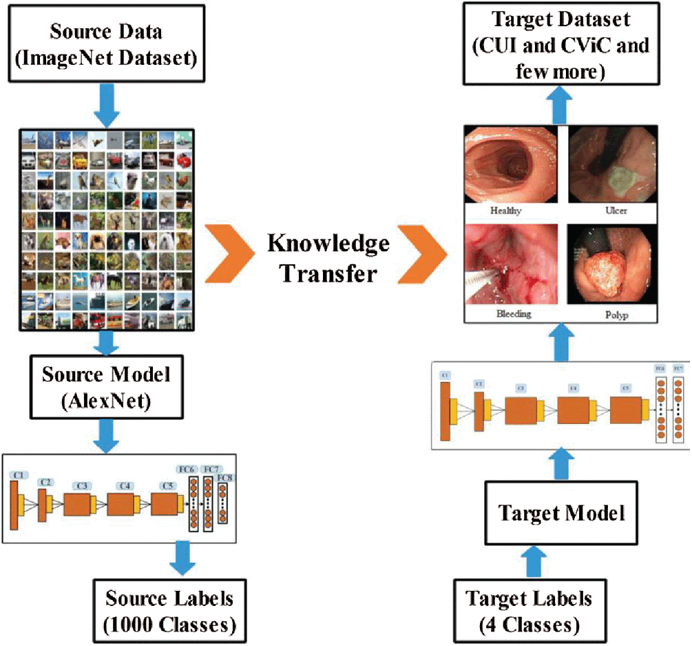
Figure 5: Transfer learning for stomach infection classification
2.3 Features Extraction & Fusion
Feature extraction is vital; the features are the object input [33]. We extracted deep learning features from layers FC6 and FC7. Mathematically, the vectors are
The resultant feature-length is
This shows that fused vector features
2.4 Modified Genetic Algorithm
A GA [34] is an evolutionary algorithm applied to identify optimal solutions among a set of original solutions. In other words, a GA is a heuristic search algorithm that organizes the best solutions into spaces. GAs involve five steps: initialization/population initialization, crossover, mutation, selection, and reproduction.
Initialization. The maximum number of iterations, population size, crossover percentage, offspring number, mutation percentage, number of mutants, and the mutation and selection rates are initialized. Here, the iteration number is 100, the population size 20, the mutation rate 0.2, the crossover rate 0.5, and the selection pressure 7.
Population Initialization. We initialize the size of the GA population (here 20). Every population is selected randomly in terms of its fused vector and evaluated using a fitness function. Here, the softmax function with the fine-k-nearest neighbor [F-KNN] method is used. Non-selected features undergo crossover and mutation.
Crossover. Crossover mirrors chromosomal behavior. A parent is used to create a child. Here, the uniform crossover rate is 0.5. Mathematically, crossover can be expressed as follows.
Here,
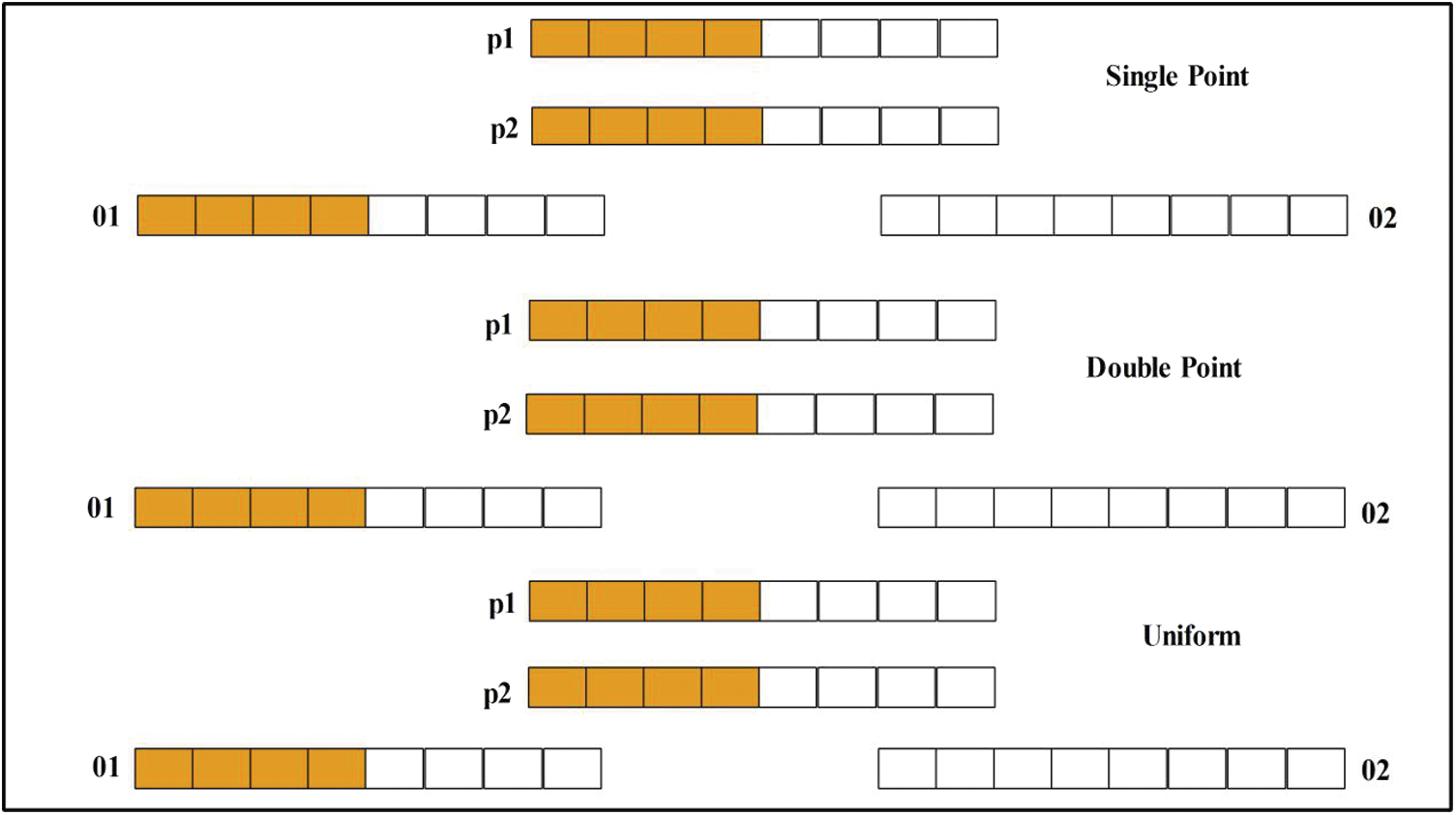
Figure 6: Architecture of crossover
Mutation. To impart unique characteristics to the offspring, one mutation is created in each offspring generated by crossover. The mutation rate was 0.2. Then, we used the Roulette Wheel (RW) [35] method to select chromosomes. The RW is based on probability.
In Eq. (16), the sorted population is
Selection and Reproduction. Crossover and mutation facilitate chromosome selection by the RW method. Thus, the selection pressure is moderate rather than high or low. All offspring engage in reproduction, and then fitness values are computed. The chromosomes are illustrated in Fig. 7. They were evaluated using the fitness function where the error rate was the measure of interest. Then, the old generation was updated.
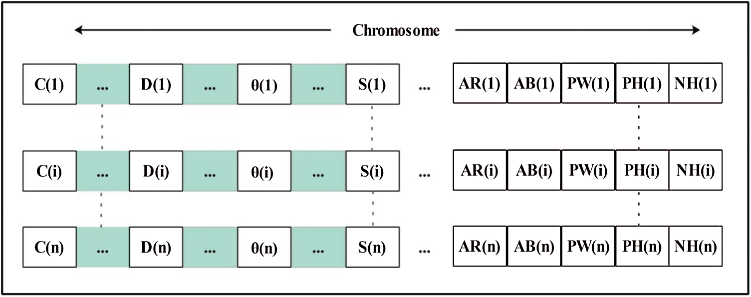
Figure 7: Demonstration of chromosomes
This process continues until no further iteration is possible. A vector has been obtained, but remains of high dimensions. To reduce the length, we added an activation function based on kurtosis. This value is computed after iteration is complete and used to compare selected features (chromosomes). Those that do not fulfill the activation criterion are discarded. Mathematically, it can be expressed as follows:
The final selected vector is passed to several machine learning classifiers for classification. In this study, the vector dimension in is
We used 4,000 WCE images and employed 10 classifiers: The Cubic SVM, Quadratic SVM, Linear SVM, Coarse Gaussian SVM, Medium Gaussian SVM, Fine KNN, Medium KNN, Weighted KNN, Cosine KNN, and Bagged Tree. Of the complete dataset, 70% was used for training and 30% for testing (10 cross-validations). We used a Core i7 CPU with 14 GB of RAM and a 4 GB graphics card. Coding employed MATLAB 2020a and Matconvent (for deep learning). We measured sensitivity, precision, the F1-score, the false-positive rate (FPR), the area under the curve (AUC), accuracy, and time.
The results are shown in Tab. 1. The highest accuracy was 99.2% (using the Cubic SVM). The sensitivity, precision, and F1-score were all 99.00%. The FPR was 0.002, the AUC was 1.00, and the (computational) time was 83.79 s. The next best accuracy was 99.6% (Quadratic SVM). The associated metrics (in the above order) were 98.75%, 99.00%, 99.00%, 0.002, 1.000, and 78.52 s, respectively. The Cosine KNN, Weighted KNN, Medium KNN, Fine KNN, MG SVM, Coarse Gaussian SVM, Linear SVM, and Bagged Tree accuracies were 97.0%, 98.0%, 96.7%, 98.9%, 98.9%, 93.3%, 96.9%, and 96.8%, respectively. The Cubic SVM scatterplot of the original test features is shown in Fig. 8. The first panel refers to the original data and the second to the Cubic SVM predictions. The good Cubic SVM performance is confirmed by the confusion matrix shown in Fig. 9. Bleeding was accurately predicted 99% of the time, as were healthy tissue and ulcers; the polyp figure was > 99%. The ROC plots of the Cubic SVM are shown in Fig. 10.
Table 1: Classification accuracy of proposed optimal feature selection algorithm (testing feature results)
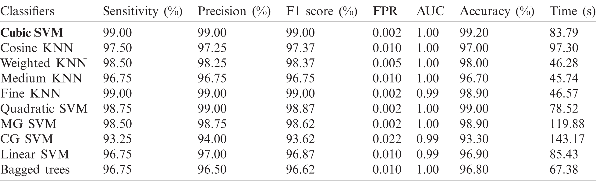
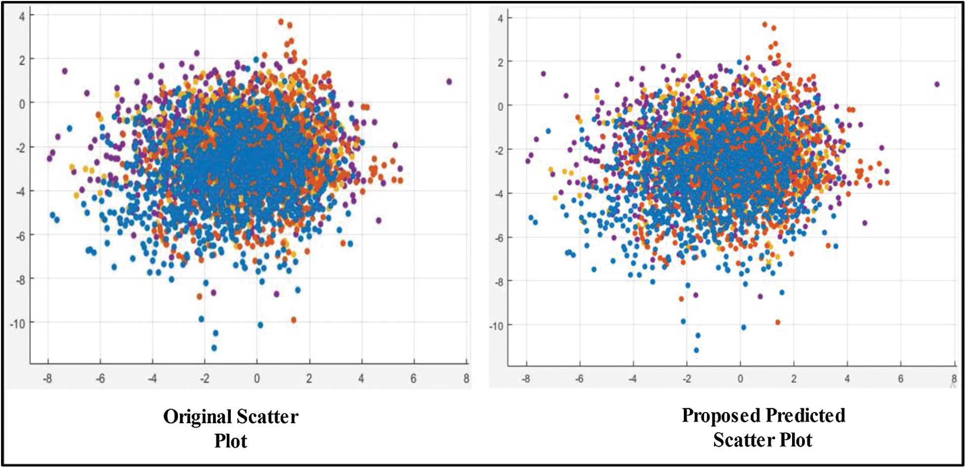
Figure 8: Scatter plot for testing features after applying GA
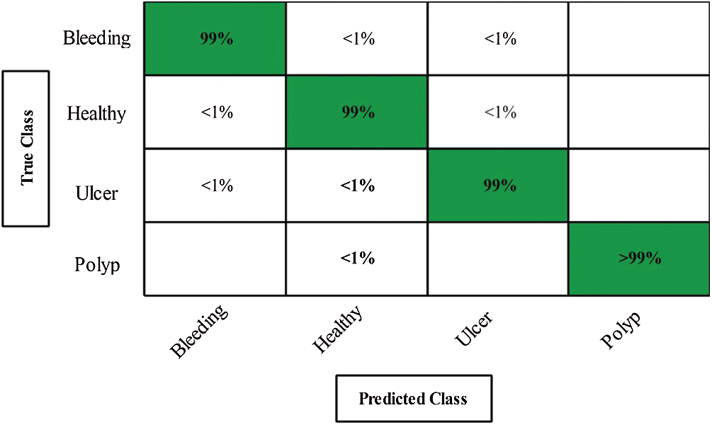
Figure 9: Confusion matrix of cubic SVM for proposed method
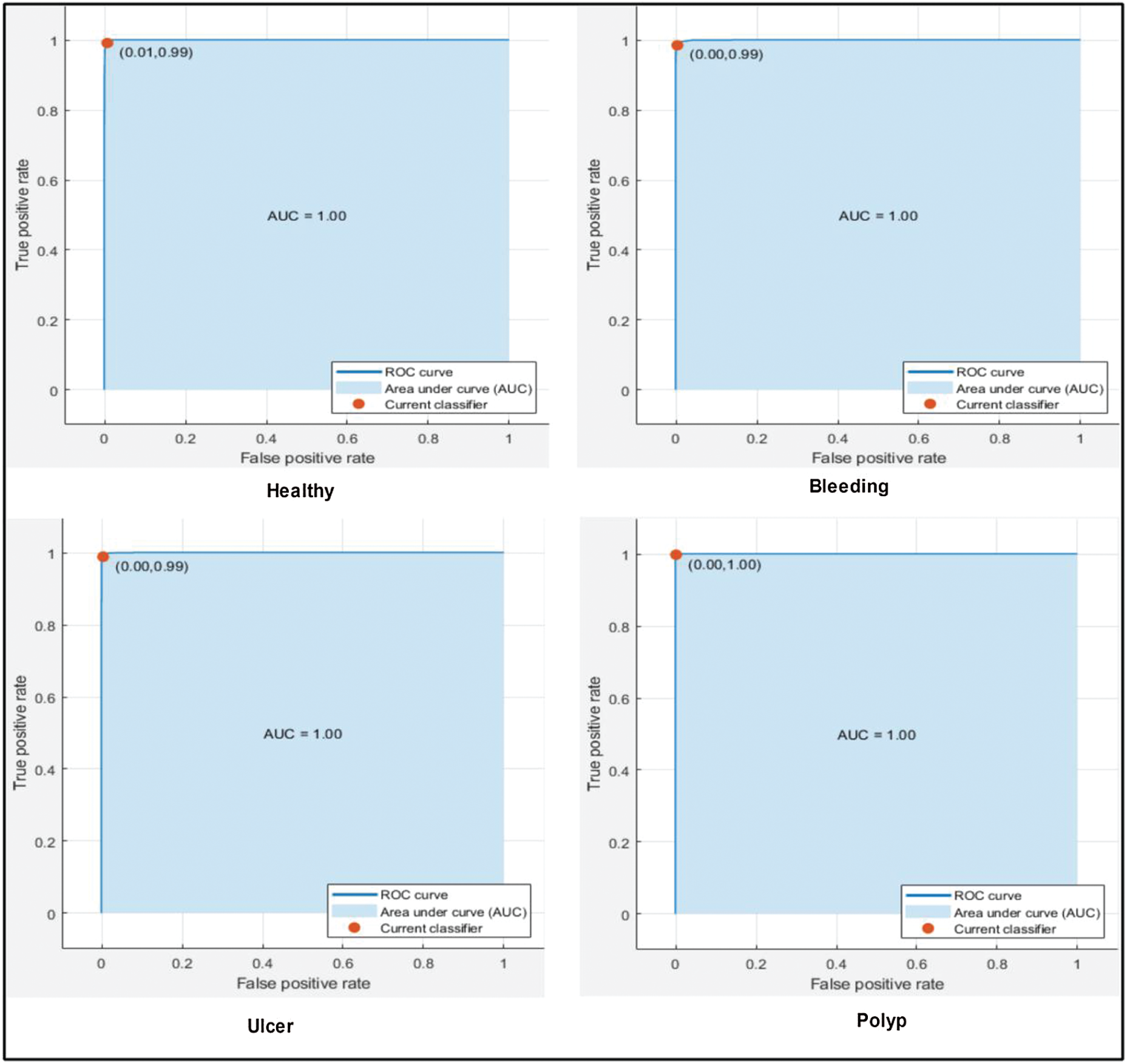
Figure 10: ROC plots for selected stomach cancer classes using cubic SVM after applying GA
Next, we applied our improved GA. The results are shown in Tab. 2. The top accuracy (99.8%) was afforded by the Cubic SVM accompanied by sensitivity of 99.00%, precision of 99.25%, F1-score of 99.12%, FPR of 0.00, AUC of 1.00, and a time of 211.90 s. The second highest accuracy was 99.0% achieved by the Fine KNN, accompanied by (in the above order) values of 99.0%, 99.25%, 99.12%, 0.00, 1.00, and 239.08 s, respectively. The Cosine KNN, Weighted KNN, Medium KNN, Quadratic SVM, MG SVM, Coarse Gaussian SVM, Linear SVM, and Bagged Tree achieved accuracies of 99.0%, 99.5%, 98.7%, 99.6%, 99.6%, 96.2%, 98.3%, and 98.3%, respectively. The Cubic SVM scatterplot of the original test features is shown in Fig. 11. The first panel refers to the original data and the second to the Cubic SVM predictions. The good Cubic SVM performance is confirmed by the confusion matrix shown in Fig. 12. In this figure, the four classes are healthy tissue, bleeding sites, ulcers, and polyps. Bleeding was accurately predicted 99% of the time, healthy tissue < 99% of the time, and ulcers and polyps > 99% of the time. The ROC plots of the Cubic SVM are shown in Fig. 13.
Table 2: Classification accuracy of proposed optimal feature selection algorithm using training features
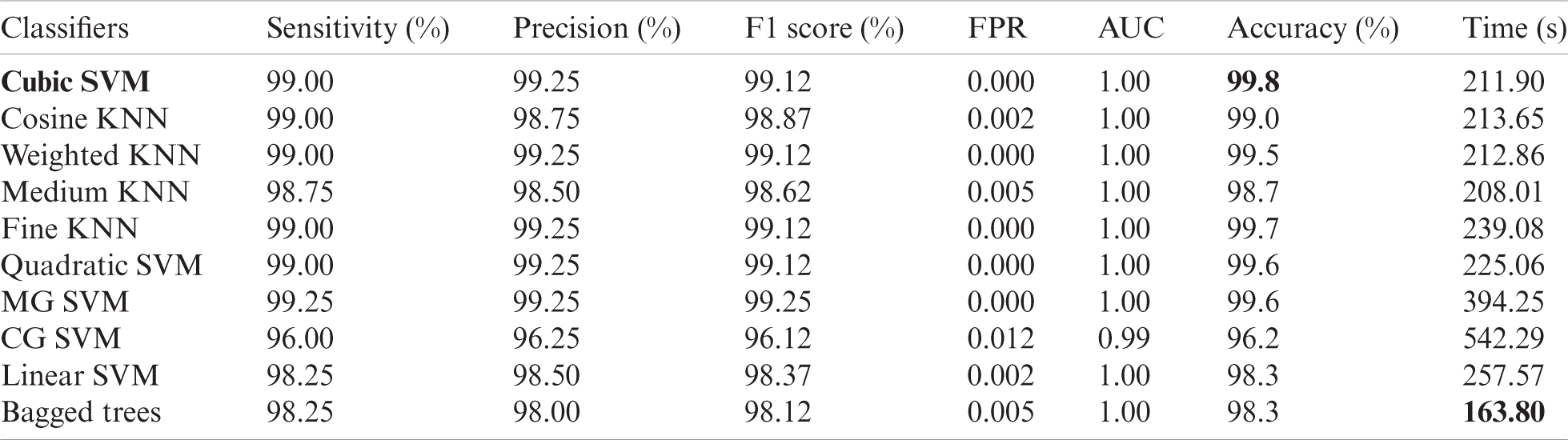
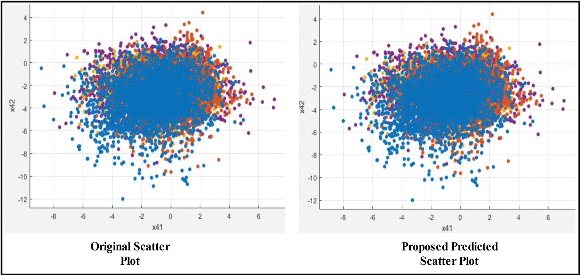
Figure 11: Scatter plot of training features after applying GA

Figure 12: Confusion matrix of CUBIC SVM
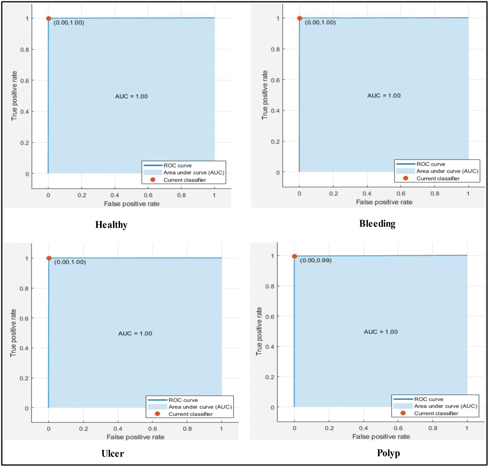
Figure 13: ROC plots for selected stomach cancer classes using cubic SVM after applying GA
3.3 Comparison with Existing Techniques
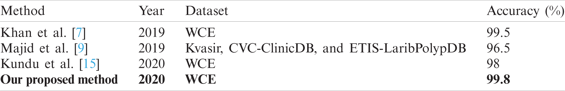
In this section, we compare the proposed method to existing techniques (Tab. 3). In a previous study [7], CNN feature extraction, fusing of different features, selection of the best features, and classification were used to detect ulcers in WCE images. The dataset was collected in the POF Hospital Wah Cantt, Pakistan; the accuracy was 99.5%. Another study [9] described handcrafted and deep CNN feature extraction from the Kvasir, CVC–ClinicDB, a private, and ETIS-Larib PolypDB datasets. The accuracy was 96.5%. In another study [15], and LSST technique using probabilistic model-fitting was used to evaluate a WCE dataset; the accuracy was 98%. Our method employs deep learning and a modified GA. We used the private dataset of the POF Hospital, and the Kvasir and CVC datasets to identify ulcers, polyps, bleeding sites, and healthy tissue. The accuracy was 99.8% and the computational time was 211.90 s. Our method outperforms the existing techniques.
Table 3: Proposed method’s accuracy compared with published techniques
We automatically identify various stomach diseases using deep learning and an improved GA. WCE image contrast is enhanced using a new color discrimination-based hybrid approach. This distinguishes diseased and healthy regions, which facilitates later feature extraction. We fine-tuned the pretrained AlexNet deep learning model by the classifications of interest. We employed transfer learning further train the AlexNet model. We fused features extracted from two layers; this improved local and global information. We removed some redundant features by modifying the GA fitness function and using kurtosis to select the best features. This improved accuracy and minimized computational time. The principal limitation of the work is that the features are of high dimension, which increases computational cost. We will resolve this problem by employing DarkNet and MobileNet (the latest deep learning models [36,37]). Before feature extraction, disease localization accelerates execution.
Acknowledgement: The authors extend their appreciation to the Deanship of Scientific Research at King Saud University for funding this work through research group NO (RG-1438-034). The authors thank the Deanship of Scientific Research and RSSU at King Saud University for their technical support.
Funding Statement: This research was supported by Korea Institute for Advancement of Technology (KIAT) grant funded by the Korea Government (MOTIE) (P0012724, The Competency Development Program for Industry Specialist) and the Soonchunhyang University Research Fund.
Conflicts of Interest: The authors declare that they have no conflicts of interest to report regarding the present study.
1. M. A. Khan, M. S. Sarfraz, M. Alhaisoni, A. A. Albesher, S. Wang et al., “StomachNet: Optimal deep learning features fusion for stomach abnormalities classification,” IEEE Access, vol. 8, pp. 197969–197981, 2020. [Google Scholar]
2. M. A. Khan, S. Kadry, M. Alhaisoni, Y. Nam, Y. Zhang et al., “Computer-aided gastrointestinal diseases analysis from wireless capsule endoscopy: A framework of best features selection,” IEEE Access, vol. 8, pp. 132850–132859, 2020. [Google Scholar]
3. A. Nema, S. K. Gupta, T. S. Dudhamal and V. Mahanta, “Transrectal ultra sonography based evidence of ksharasutra therapy for fistula-in-ano-a case series,” Journal of Ayurveda and Integrative Medicine, vol. 8, no. 2, pp. 113–121, 2017. [Google Scholar]
4. M. E. Morrison, J. M. Joseph, S. E. McCann, L. Tang, H. M. Almohanna et al., “Cruciferous vegetable consumption and stomach cancer: A case-control study,” Nutrition and Cancer, vol. 72, no. 1, pp. 52–61, 2020. [Google Scholar]
5. T. Nishizawa, O. Toyoshima, R. Kondo, K. Sekiba, Y. Tsuji et al., “The simplified Kyoto classification score is consistent with the ABC method of classification as a grading system for endoscopic gastritis,” Journal of Clinical Biochemistry and Nutrition, vol. 4, pp. 20–41, 2020. [Google Scholar]
6. D. Surangsrirat, A. Tongkratoke, S. Samphanyuth, T. Sununtachaikul and A. Pramuanjaroenkij, “Development in rubber preparation for endoscopic training simulator,” Advances in Materials Science and Engineering, vol. 2016, no. 1, pp. 8650631, 2016. [Google Scholar]
7. M. A. Khan, M. Sharif, T. Akram, M. Yasmin and R. S. Nayak, “Stomach deformities recognition using rank-based deep features selection,” Journal of Medical Systems, vol. 43, no. 12, pp. 329, 2019. [Google Scholar]
8. A. Liaqat, M. A. Khan, M. Sharif, M. Mittal, T. Saba et al., “Gastric tract infections detection and classification from wireless capsule endoscopy using computer vision techniques: A review,” Current Medical Imaging, vol. 2, pp. 1–31, 2020. [Google Scholar]
9. A. Majid, M. A. Khan, M. Yasmin, A. Rehman, A. Yousafzai et al., “Classification of stomach infections: A paradigm of convolutional neural network along with classical features fusion and selection,” Microscopy Research and Technique, vol. 83, no. 5, pp. 562–576, 2020. [Google Scholar]
10. M. A. Khan, M. A. Khan, F. Ahmed, M. Mittal, L. M. Goyal et al., “Gastrointestinal diseases segmentation and classification based on duo-deep architectures,” Pattern Recognition Letters, vol. 131, pp. 193–204, 2020. [Google Scholar]
11. A. Yasar, I. Saritas and H. Korkmaz, “Computer-aided diagnosis system for detection of stomach cancer with image processing techniques,” Journal of Medical Systems, vol. 43, no. 4, pp. 99, 2019. [Google Scholar]
12. P. Afshar, S. Heidarian, F. Naderkhani, A. Oikonomou, K. N. Plataniotis et al., “Covid-caps: A capsule network-based framework for identification of covid-19 cases from X-ray images,” Pattern Recognition Letters,vol. 138, pp. 638–643, 2020. [Google Scholar]
13. M. I. Sharif, J. P. Li, M. A. Khan and M. A. Saleem, “Active deep neural network features selection for segmentation and recognition of brain tumors using MRI images,” Pattern Recognition Letters, vol. 129, no. 10, pp. 181–189, 2020. [Google Scholar]
14. J. S. Cai, H.-Y. Chen, J. Y. Chen, Y. F. Lu, J. Z. Sun et al., “Reduced field-of-view diffusion-weighted imaging (DWI) in patients with gastric cancer: Comparison with conventional DWI techniques at 3.0 T: A preliminary study,” Medicine, vol. 99, pp. 1–7, 2020. [Google Scholar]
15. A. K. Kundu, S. A. Fattah and K. A. Wahid, “Least square saliency transformation of capsule endoscopy images for PDF model based multiple gastrointestinal disease classification,” IEEE Access, vol. 8, pp. 58509–58521, 2020. [Google Scholar]
16. M. A. Khan, M. Rashid, M. Sharif, K. Javed and T. Akram, “Classification of gastrointestinal diseases of stomach from WCE using improved saliency-based method and discriminant features selection,” Multimedia Tools and Applications, vol. 78, no. 19, pp. 27743–27770, 2019. [Google Scholar]
17. H. Alaskar, A. Hussain, N. Al-Aseem, P. Liatsis and D. Al-Jumeily, “Application of convolutional neural networks for automated ulcer detection in wireless capsule endoscopy images,” Sensors, vol. 19, no. 6, pp. 1265, 2019. [Google Scholar]
18. Q. Wang, H. Fan and Y. Tang, “Computer-aided WCE diagnosis using convolutional neural network and label transfer,” in 2019 IEEE 9th Annual Int. Conf. on CYBER Technology in Automation, Control, and Intelligent Systems, Suzhou, China, pp. 581–585, 2019. [Google Scholar]
19. S. Wang, Y. Xing, L. Zhang, H. Gao and H. Zhang, “Deep convolutional neural network for ulcer recognition in wireless capsule endoscopy: Experimental feasibility and optimization,” Computational and Mathematical Methods in Medicine, vol. 2019, pp. 21–33, 2019. [Google Scholar]
20. A. Rehman, M. A. Khan, T. Saba, Z. Mehmood, U. Tariq et al., “Microscopic brain tumor detection and classification using 3D CNN and feature selection architecture,” Microscopy Research and Technique, vol. 2, pp. 1–21, 2020. [Google Scholar]
21. M. A. Khan, M. Qasim, H. M. J. Lodhi, M. Nazir, K. Javed et al., “Automated design for recognition of blood cells diseases from hematopathology using classical features selection and ELM,” Microscopy Research and Technique, vol. 1, pp. 1–18, 2020. [Google Scholar]
22. M. A. Khan, M. Sharif, T. Akram, S. A. C. Bukhari and R. S. Nayak, “Developed newton-raphson based deep features selection framework for skin lesion recognition,” Pattern Recognition Letters, vol. 129, no. 4/5, pp. 293–303, 2020. [Google Scholar]
23. K. He, J. Sun and X. Tang, “Single image haze removal using dark channel prior,” IEEE Transactions on Pattern Analysis and Machine Intelligence, vol. 33, pp. 2341–2353, 2010. [Google Scholar]
24. M. S. Iraji and A. Yavari, “Skin color segmentation in fuzzy YCBCR color space with the mamdani inference,” American Journal of Scientific Research, vol. 2011, pp. 131–137, 2011. [Google Scholar]
25. M. A. Khan, I. Ashraf, M. Alhaisoni, R. Damaševičius, R. Scherer et al., “Multimodal brain tumor classification using deep learning and robust feature selection: A machine learning application for radiologists,” Diagnostics, vol. 10, pp. 565, 2020. [Google Scholar]
26. M. Rashid, M. A. Khan, M. Alhaisoni, S.-H. Wang, S. R. Naqvi et al., “A sustainable deep learning framework for object recognition using multi-layers deep features fusion and selection,” Sustainability, vol. 12, pp. 5037, 2020. [Google Scholar]
27. A. Adeel, M. A. Khan, T. Akram, A. Sharif, M. Yasmin et al., “Entropy-controlled deep features selection framework for grape leaf diseases recognition,” Expert Systems, vol. 2, pp. 1–28, 2020. [Google Scholar]
28. M. A. Khan, Y. D. Zhang, S. A. Khan, M. Attique, A. Rehman et al., “A resource conscious human action recognition framework using 26-layered deep convolutional neural network,” Multimedia Tools and Applications, vol. 3, pp. 1–23, 2020. [Google Scholar]
29. H. Arshad, M. A. Khan, M. I. Sharif, M. Yasmin, J. M. R. Tavares et al., “A multilevel paradigm for deep convolutional neural network features selection with an application to human gait recognition,” Expert Systems, vol. 21, no. 3, pp. e12541, 2020. [Google Scholar]
30. A. Krizhevsky, I. Sutskever and G. E. Hinton, “Imagenet classification with deep convolutional neural networks,” Communications of the ACM, vol. 60, no. 6, pp. 84–90, 2017. [Google Scholar]
31. R. Wang, J. Xu and T. X. Han, “Object instance detection with pruned Alexnet and extended training data,” Signal Processing: Image Communication, vol. 70, no. 4, pp. 145–156, 2019. [Google Scholar]
32. S. J. Pan and Q. Yang, “A survey on transfer learning,” IEEE Transactions on Knowledge and Data Engineering, vol. 22, no. 10, pp. 1345–1359, 2009. [Google Scholar]
33. M. Rashid, M. A. Khan, M. Sharif, M. Raza, M. M. Sarfraz et al., “Object detection and classification: A joint selection and fusion strategy of deep convolutional neural network and SIFT point features,” Multimedia Tools and Applications, vol. 78, no. 12, pp. 15751–15777, 2019. [Google Scholar]
34. B. Bhanu and Y. Lin, “Genetic algorithm based feature selection for target detection in SAR images,” Image and Vision Computing, vol. 21, no. 7, pp. 591–608, 2003. [Google Scholar]
35. A. Lipowski and D. Lipowska, “Roulette-wheel selection via stochastic acceptance,” Physica A: Statistical Mechanics and Its Applications, vol. 391, no. 6, pp. 2193–2196, 2012. [Google Scholar]
36. S. H. Wang, V. V. Govindaraj, J. M. Górriz, X. Zhang and Y. D. Zhang, “Covid-19 classification by FGCNet with deep feature fusion from graph convolutional network and convolutional neural network,” Information Fusion, vol. 67, pp. 208–229, 2020. [Google Scholar]
37. Y. D. Zhang, S. C. Satapathy, S. Liu and G. R. Li, “A five-layer deep convolutional neural network with stochastic pooling for chest CT-based COVID-19 diagnosis,” Machine Vision and Applications, vol. 32, no. 1, pp. 1–13, 2020. [Google Scholar]
 | This work is licensed under a Creative Commons Attribution 4.0 International License, which permits unrestricted use, distribution, and reproduction in any medium, provided the original work is properly cited. |