DOI:10.32604/cmc.2021.015906
| Computers, Materials & Continua DOI:10.32604/cmc.2021.015906 | |
| Article |
Intelligent Autonomous-Robot Control for Medical Applications
1College of Engineering, Muzahimiyah Branch, King Saud University, Riyadh, 11451, Saudi Arabia
2Laboratory for Analysis, Conception and Control of Systems, Department of Electrical Engineering, National Engineering School of Tunis, Tunis El Manar University, 1002, Tunisia
3King Abdulaziz City for Science and Technology, Riyadh, 12354, Saudi Arabia
4College of Computing and Information Technology, University of Bisha, Bisha, 67714, Saudi Arabia
*Corresponding Author: Haykel Marouani. Email: hmarouani@ksu.edu.sa
Received: 13 December 2020; Accepted: 28 February 2021
Abstract: The COVID-19 pandemic has shown that there is a lack of healthcare facilities to cope with a pandemic. This has also underscored the immediate need to rapidly develop hospitals capable of dealing with infectious patients and to rapidly change in supply lines to manufacture the prescription goods (including medicines) that is needed to prevent infection and treatment for infected patients. The COVID-19 has shown the utility of intelligent autonomous robots that assist human efforts to combat a pandemic. The artificial intelligence based on neural networks and deep learning can help to fight COVID-19 in many ways, particularly in the control of autonomous medic robots. Health officials aim to curb the spread of COVID-19 among medical, nursing staff and patients by using intelligent robots. We propose an advanced controller for a service robot to be used in hospitals. This type of robot is deployed to deliver food and dispense medications to individual patients. An autonomous line-follower robot that can sense and follow a line drawn on the floor and drive through the rooms of patients with control of its direction. These criteria were met by using two controllers simultaneously: a deep neural network controller to predict the trajectory of movement and a proportional-integral-derivative (PID) controller for automatic steering and speed control.
Keywords: Autonomous medic robots; PID control; neural network control system; real-time implementation; navigation environment; differential drive system
The use of robotics, automation applications, and artificial intelligence in public healthcare is growing daily [1–3]. Robots support doctors and medical personnel to perform complicated functions with accuracy, and to reduce the workload of medical staff, improving the efficacy of healthcare services [4]. To minimize the spread of COVID-19, several work functions have been allocated to robots, such as cleaning and food processing jobs in contaminated areas [5]. In hospitals, service robots are versions of mobile robots with high payload capability but restricted degrees of freedom (Fig. 1). However, surgical robots are precise, flexible, and reliable systems with a minimal error margin, typically within millimeters [6,7].
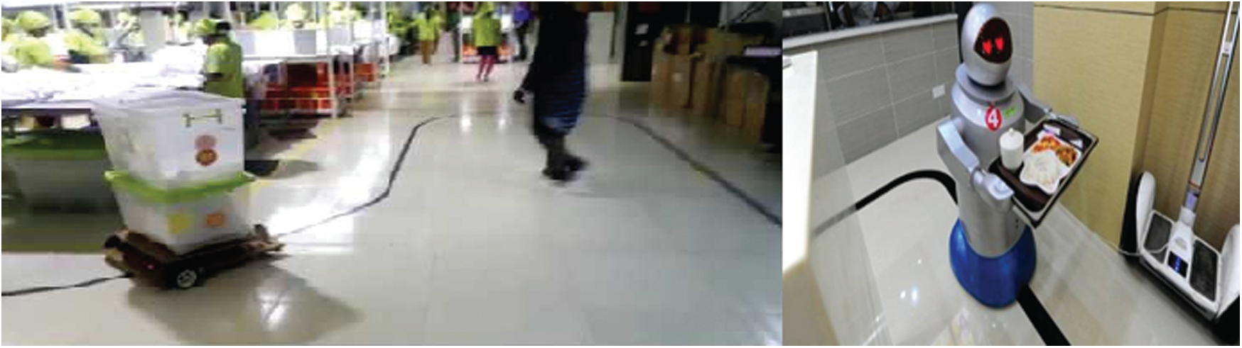
Figure 1: Line-follower service robots
Mobile robots are machines controlled by software and integrated sensors, including infrared, ultrasonic, webcam, GPS, and magnetic sensors, and they can move from one location to another to perform complex tasks [8]. Wheels and DC motors are used to move robots [9]. In addition to their use in healthcare, mobile robots are used in agricultural, industrial, military, and search and rescue applications, helping humans to accomplish complicated tasks [10]. Line-follower robots can be used in many industrial logistics applications, such as the transport of heavy and dangerous materials, the agriculture sector, and library inventory management systems. These robots are also capable of monitoring patients in hospitals and warning doctors of concerning symptoms [11].
A growing number of researchers have focused on smart-vehicle navigation because traditional tracking techniques are limited due to the environmental instability under which a vehicle moves. Therefore, intelligent control mechanisms, such as neural networks, are needed. They solve the problem of vehicle navigation by using their ability to learn the non-linear relationship between input and sensor values. A combination of computer vision techniques and machine learning algorithms is necessary for autonomous robots to develop “true consciousness” [12]. Several attempts have been made to improve low-cost autonomous cars using different neural network configurations. For example, the use of convolutional neural networks (CNNs) has been proposed for self-driving vehicles [13]. A collision prediction system has been constructed that combines a CNN with a method of stopping a robot in the vicinity of the target point while avoiding a moving obstacle [14]. CNNs have also been proposed for autonomous driving control systems to keep robots in their allocated lanes [15]. A multilayer perceptron network, which was implemented on a PC with an Intel Pentium 350 MHz processor, has been used for mobile-robot motion planning [16]. In another study, the problem of navigating a mobile robot was solved using a local neural network model [17].
Several motion control methods have been proposed for autonomous robots: proportional-integral-derivative (PID) control, fuzzy control, neural network control, and combinations of these control algorithms [18]. PID control is used by most motion control applications, and PID control methods have been extended with deep-learning techniques to achieve better performance and higher adaptability. High-end robotics with dynamic and reasonably accurate movement often require these control algorithms for operation. For example, a fuzzy PID controller has been used for a differential drive autonomous mobile-robot trajectory application [19]. A PID controller has also been designed to enable a laser sensor-based mobile robot to detect obstacles and avoid them [20].
In this paper, we outline the construction of a low-cost PID controller combined with a multilayer feed-forward network based on a back-propagation training algorithm using the Arduino controller board for the smooth control of an autonomous line-follower robot.
2 Autonomous Line-Follower Robot Architecture
In this section, the architecture and system block diagram for the line-follower robot are described. First, a suitable configuration was selected to develop a line-follower robot using three infrared sensors connected through the Arduino Uno microcontroller board to the motor driver integrated circuit (IC). This configuration is illustrated in the block diagram shown in Fig. 2.
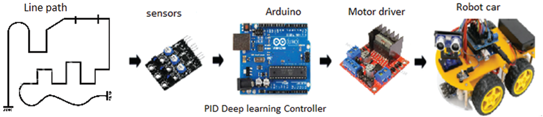
Figure 2: Block diagram of the medic line-follower robot
Implementing the system on the Arduino Uno ensured that the robot moved in the desired direction; the infrared sensors were read for line detection; error was predicted; the speed of the left and the right motors was determined using a PID controller and the predicted error; and the line-follower robot operated by reading the infrared sensors and controlling the four DC motors.
The proposed autonomous-robot design (Fig. 3) can easily be modified and adapted to new research studies. The physical appearance of the robot was evaluated, and its design was based on several criteria, including functionality, material availability, and mobility.
Seven part types were used in the construction of the robot:
1. Four wheels.
2. Four DC motors.
3. Two base structures.
4. A controller board based on the Arduino ATmega 32 board.
5. An L298N IC circuit for DC-motor driving.
6. An expansion board.
7. Line-tracking module.
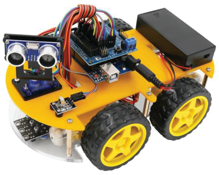
Figure 3: Medic line-follower robot prototype
2.2 Arduino Uno Microcontroller
The Arduino Uno is a microcontroller board based on the ATmega328P (Fig. 4). It has 14 digital I/O pins, six analog inputs that can be used as pulse width modulation (PWM) outputs, a USB connector, a power jack, an ICSP header, a reset button, and a 16-MHz quartz crystal. The Arduino microcontroller board is suitable for driving a PWM signal for the DC motor [21].
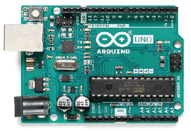
Figure 4: Arduino Uno based on the ATmega328P
The line-tracking sensor used is capable of detecting white lines on black, and black lines on white (Fig. 5). The single line-tracking signal provides a stable output TTL signal for more accurate and more stable line tracking. Multi-channel operation can easily be achieved by installing the necessary line-tracking robot sensors [22].
Specifications:
Power Supply: +5 V, operating Current: < 10 mA
Operating temperature range: 0
Output Interface: Three-wire interface (1—signal, 2—power, and 3—power supply negative) output Level: TTL level.
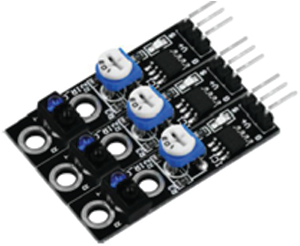
Figure 5: Tracking sensor
The L298N motor driver, which consists of two complete H-bridge circuits, is capable of driving a pair of DC motors. This function makes it suitable for use in robotics because most robots run on two or four driven wheels with a power current of up to 2A and a voltage from 5 to 35V DC. Fig. 6 shows the pin assignments for the L298N dual H-bridge module. IN1 and IN2 on the L298N board are used to control the direction. The PWM signal was sent to the Enable pin of the L298N board, which drives the motor [22].

Figure 6: L298N IC motor driver
Fig. 7 shows a diagram indicating the wire connections used for the design and implementation of the mobile robot. This diagram includes the embedded system, line-tracking sensors, DC motors, and L298 IC circuit for driving the motors.
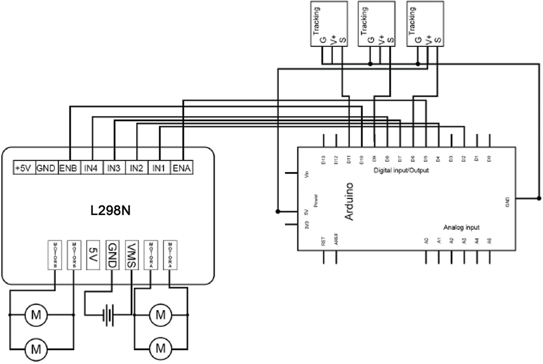
Figure 7: Connection wires
3 Neural Network-Based PID Controller for a Line-Follower Robot
A neural network-based PID controller was designed to control the robot. The sensors were numbered from left to right. An error value of zero referred to the robot being precisely on the center of the line. A positive error value meant that the robot had deviated to the left, and a negative error value meant that the robot had deviated to the right. The error value can be a maximum of

Figure 8: Errors and sensor positions
The primary advantage of this approach is that the three sensor readings are replaced with a single error term, which can be fed to the controller to compute the motor speeds so that the error term becomes zero. The output of the tracking line sensor array is fed to the neural network, which calculates and estimates the error term from the sensor values.
The estimated error input was used by the PID controller to generate new output values. The output value was used to determine the left speed and right speed for the two motors on the line-follower robot.
Fig. 9 shows the control algorithm used for the line-follower robot.
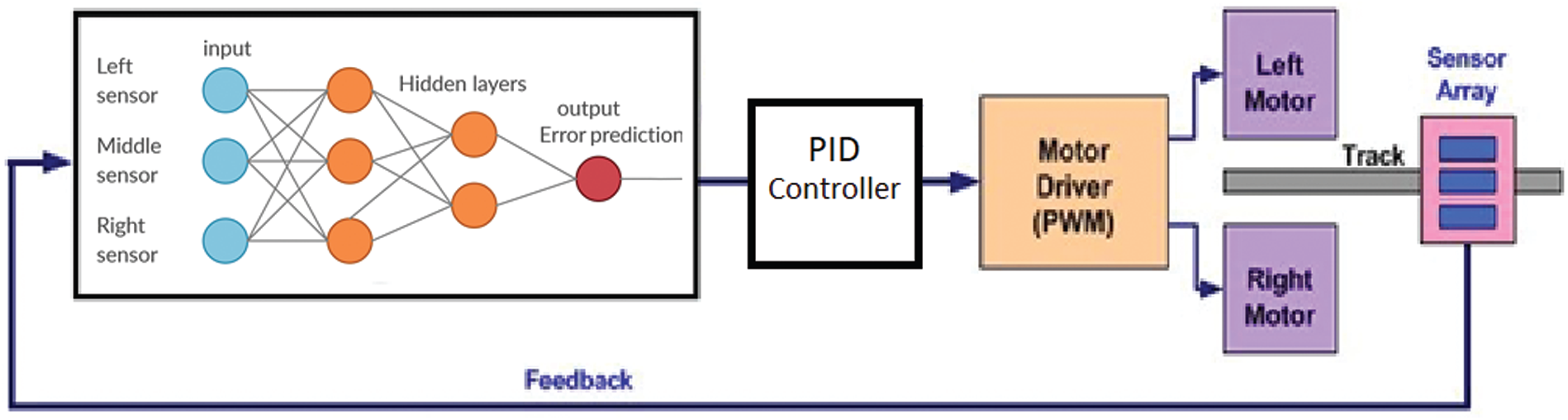
Figure 9: Mobile robot motion-control-based proportional-integral-derivative (PID) neural network controller
The objective of a PID controller is to keep an input variable close to the desired set-point by adjusting an output. Its performance can be “tuned” by adjusting three parameters: KP, KI, and KD. The well-known PID controller equation is shown here in continuous form:
where Kp, Ki, and Kd refer to proportional, integral, and derivative gain constants, respectively.
For implementation in a discrete form, the controller equation is modified using the backward Euler method for numerical integration, as in
where u(kT) and e(kT) are control and error signals in discrete time at T sampling time.
The PID controller determines both the left and right motor speeds following a predicted error measurement of the sensor. The PID controller generates a control signal (PID value), which is used to determine the left and right speeds of the robot wheels. This is a differential drive system, in which a left turn can be executed if the speed of the left motor is reduced, and a right turn is executed if the speed of the right motor is reduced. Right_Speed and Left_Speed are calculated using Eq. (3):
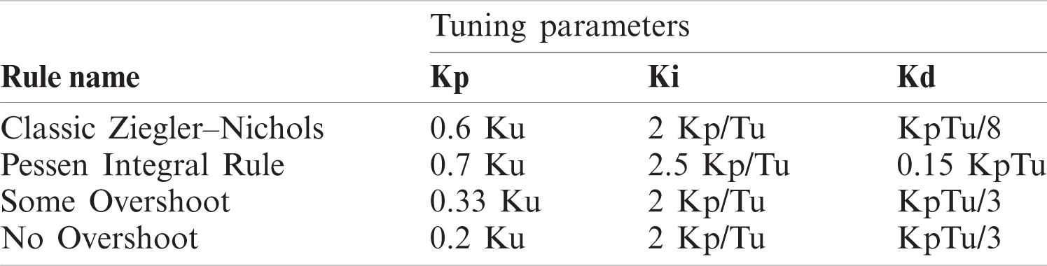
Right_Speed and Left_Speed are used to control the duty cycle of the PWM applied at the input pins of the motor driver IC. PID constants (Kp, Ki, Kd) were obtained using the Ziegler–Nichols tuning method (Tab. 1) [23]. Initially, the Ki and Kd of the system were set to 0. Kp was then increased from 0 until it reached the ultimate gain Ku, and at this point, the robot continuously oscillated. Ku and Tu (oscillation period) are then used to tune the PID (see Tab. 1).
Table 1: Proportional-integral-derivative tuning parameters for controlling a mobile robot
After substantial testing, using a classical PID controller was deemed unsuitable for the line-follower robot because of the changes in line curvature. Therefore, only the last three error values were tallied instead of adding all the previous values to solve this problem. The modified controller equation is provided in Eq. (4):
This technique provides a satisfactory performance for path tracking.
3.2 Artificial Neural Network Mathematical Model
An artificial neural network (ANN) is a computing system that consists of many simple but highly interconnected processing elements. These elements are processed by variations in external inputs. The ANN structure presented in this work was built using multiple weighted hidden layers, which were supervised by a feed-forward network using a back-propagation algorithm. This method is widely used in many applications [24]. ANNs are best suited to human-like operations, such as image processing, speech recognition, robotic control, and power system protection and control management. An ANN can be compared to a human brain. The human brain operates rapidly and consists of many neurons or nodes. Each signal or bit of information travels through a neuron, where it is processed, calculated, manipulated, and then transferred to the next neuron cell. The overall processing speed of each neuron or node may be slow, but the overall network is very fast and efficient.
The first layers used in the ANN are the input layer and the highest layer, which is the output layer. Each bit of information is processed through the hidden layers (intermediate layers) and output layers. The signals or information data are manipulated, calculated, and processed in each layer, before being transferred to the respective network layers. When information is processed through layers or nodes in an ANN, more efficient results can be obtained when the number of hidden layers increases. The ANN operates through these layers and calculates and overwrites the results as it is trained with input data. This makes the entire network not only efficient but also capable of predicting future outcomes and making necessary decisions. This is why ANNs are often compared to the neuron cells of the human brain.
The ANN developed in this study consists of three inputs or neurons (Fig. 10). The first input is dedicated to the left sensor, the second input is dedicated to the middle sensor, and the third input is dedicated to the right sensor. Following best practices, the first hidden layer is composed of the same number of neurons as the input layer. The second hidden layer comprises two neurons, and the output layer comprises one neuron for error prediction. The hidden layers use a sigmoid function as the activation function, and the output layer uses a linear function.

Figure 10: Neural network structure for controlling a mobile robot
Three-layered feed-forward networks were supervised by the back-propagation algorithm in the ANN. Therefore, three functions needed to be constructed: one for the inputs to the first hidden layers, another for the first hidden layer to the second hidden layer, and a third for the hidden layers to output layers or targets. Fig. 11 shows a block diagram illustrating the equations of the final output.

Figure 11: Neural network equations
4 Implementation of PID Neural Network Controller
The ANN algorithm that was developed and implemented in an embedded system for the proposed mobile robot was programmed using C language.
There are some challenges associated with the implementation of an ANN in a very small system. These challenges were more significant back in the era of inexpensive microcontrollers and hobbyist boards. However, Arduinos, like so many of today’s boards, are capable of quickly completing their required tasks.
The Arduino Uno used in this work is based on Atmel’s ATmega328P microcontroller. Its 2K of SRAM is adequate for a sample network with three inputs, five hidden cells, and one output. By leveraging the Arduino’s GCC language support for multidimensional arrays and floating-point math, the programming process becomes very manageable.
The neural network architecture and algorithm design apprenticeship are monitored offline by the Keras Python library.
4.1 ANN Implementation on Arduino
A single neuron received an input (In) and produced an output activation (Out). The activation function calculated the neuron’s output based on the sum of the weighted connections feeding that neuron. The most common activation function, which is called the sigmoid function, is the following:
To compute the hidden unit’s activations, we used the following C code:
To compute the output units’ activations, we used the following C code:
4.2 Implementation of PID Controller on Arduino
We used the code below to implement the digital PID controller.
void calculatePID( )
{
P = error;
I = I + error;
D = error-previousError;
PIDvalue = (Kp * P) + (Ki * I) + (Kd * D);
previousError = error;
}
The neural network architecture and algorithm design apprenticeship were monitored offline by Keras.
4.3 Implementation of the Proposed Neural Network Using Python and Keras
Keras is a powerful and easy-to-use Python library for developing and evaluating deep-learning models. It wraps around the numerical computation libraries Theano and TensorFlow and allows users to define and train neural network models using a few short lines of code.
1-The random number generator was initialized with a fixed seed value. In this way, the same code was run repeatedly, and the same result was obtained.
The code:
from keras.models import Sequential
from keras.layers import Dense
import numpy
numpy.random.seed(7)
2-The models in Keras are defined as a sequence of layers. A fully-connected network structure with three layers was used. Fully-connected layers were defined using the Dense class.
The first layer was created with the input_dim argument by setting it to three for the three input variables.
The number of neurons in the layer was specified as the first argument, and the activation function was specified using the activation argument.
The sigmoid activation function was used for all layers.
The first hidden layer had three neurons and expected three input variables (e.g.,
The code:
model = Sequential ( )
model.add(Dense(3, input_dim = 3, activation = ‘sigmoid’, use_bias = False))
model.add(Dense(2, activation = ‘sigmoid’, use_bias = False))
model.add(Dense(1, activation = ‘linear’, use_bias = False))
3-Once the model is defined, it can be compiled. The loss function must be specified to evaluate a set of weights. The optimizer is used to search through different weights in the network. For the case being evaluated, the mse loss and the rmsprop algorithm were used.
The code:
# Compile model
model.compile(loss=’mse’, optimizer=’RMSprop’, metrics=[rmse])
The proposed model can be trained or fitted to the loaded data by calling the fit () function. The training process runs for a fixed number of iterations through a dataset called epochs. The batch size is the number of instances evaluated before performing a weight update in the network using trial and error.
The code:
# Fit the model
model.fit(X, Y, epochs = 10000, batch_size = 10)
The proposed neural network was trained for the entire dataset, and network performance was obtained for the same dataset.
The code:
# evaluate the model
scores = model.evaluate(X, Y)
The complete code
from keras.models import Sequential
from keras.layers import Dense
import numpy
from keras import backend
# from sklearn.model_selection import train_test_split
# from matplotlib import pyplot
# fix random seed for reproducibility
numpy.random.seed(7)
def rmse(y_true, y_pred):
return backend.sqrt(backend.mean(backend.square(y_pred - y_true), axis = −1))
# # split into input (X) and output (Y) variables
X = numpy.loadtxt(’input_31.csv’, delimiter=’,’)
Y = numpy.loadtxt(’output_31.csv’, delimiter=’,’)
#(trainX, testX, trainY, testY) = train_test_split(X, Y, test_size = 0.25, random_state = 6)
# create model
model = Sequential ()
model.add(Dense(3, input_dim = 3, activation=’sigmoid’,use_bias=False))
model.add(Dense(2, activation=’sigmoid’,use_bias=False))
model.add(Dense(1, activation=’linear’,use_bias=False))# Compile model
model.compile(loss=’mse’, optimizer=’RMSprop’, metrics=[rmse])
# Fit the model
model.fit(X, Y, epochs = 10000)
# evaluate the model
#result = model.predict(testX)
#print(result- testY)
scores = model.evaluate(X, Y)
Keras was used to train the proposed ANN according to specific sensor positions placed on the path line. These sensor positions are shown in Fig. 8 and listed in Tab. 2.
Table 2: Follower-logic target/neural network manual training data
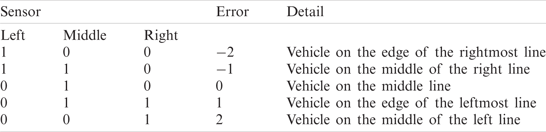
After running 1000 iterations with a decaying learning rate, the weight of each dense was found with root-mean-square error rmse = 0.13%.
The weights connecting the input layer to the hidden layer were stored in a dense_1 matrix with three rows and 10 columns.
dense_1
• [ 1.5360345, −3.6838768, −1.076581],
• [ −1.1123676, −2.4534192, 1.8363825],
• [ −3.039003, 1.5306051, 2.718451]
dense_2
• [ −2.8450463, 1.5029238],
• [3.0052474, −0.7608043],
• [ −0.91276926, −2.0846417]
dense_3
• [ 2.7599642],
• [ −3.3178754]
A comparison between real targets and the predictions calculated by Keras is presented in Tab. 3.
Table 3: Comparison between real targets and predictions calculated by Keras
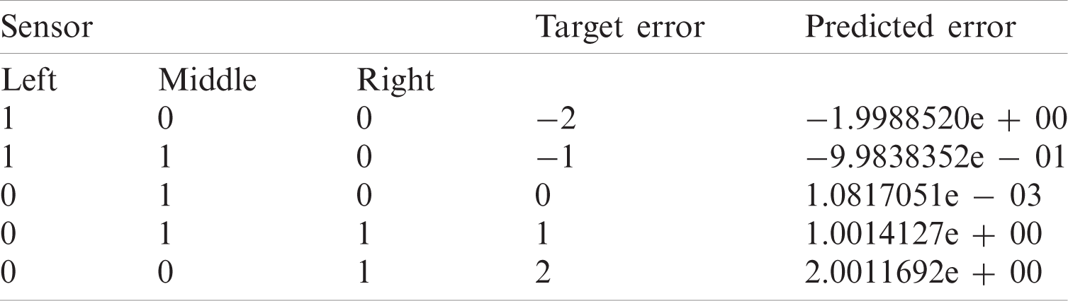
The vehicle with the trained neural network controller was successfully tested on several paths. We found that its speed varied to cope with real situations, and the robot moved faster on a straight path and reduced its speed on curves.
We developed a mobile-robot platform with a fixed four-wheel configuration chassis and a combined PID and deep-learning controller to guarantee a smooth tracking line. We found that the proposed method is well suited to mobile robots, because they are capable of operating with imprecise information. More advanced controller-based CNNs can be developed in the future.
Acknowledgement: The authors would like to extend their sincere appreciation to the Deanship of Scientific Research at King Saud University for its funding of this research through the Research Group No. RG-1439/007.
Funding Statement: The authors received funding for this research through Research Group No. RG-1439/007.
Conflicts of Interest: The authors declare that they have no conflicts of interest to report regarding the present study.
1. G. Z. Yang, B. J. Nelson, R. R. Murphy, H. Choset, H. Christensen et al., “The role of robotics in managing public health and infectious diseases,” Science Robotics, vol. 5, no. 40, pp. 1–2, 2020. [Google Scholar]
2. K. Chakraborty, S. Bhatia, S. Bhattacharyya, J. Platos, R. Bag et al., “Sentiment analysis of COVID-19 tweets by deep learning classifiers—A study to show how popularity is affecting accuracy in social media,” Applied Soft Computing, vol. 97, pp. 106754, 2020. [Google Scholar]
3. K. Dev, A. S. Khowaja, A. S. Bist, V. Saini and S. Bhatia, “Triage of potential COVID-19 patients from chest X-ray images using hierarchical convolutional networks,” Neural Computing and Applications, 2020. [Google Scholar]
4. R. H. Taylor, A. Menciassi, G. Fichtinger, P. Fiorini, P. Dario et al., “Medical robotics and computer-integrated surgery,” in Springer Handbook of Robotics, Berlin, Germany: Springer, pp. 1657–1684, 2016. [Google Scholar]
5. K. J. Vänni, S. E. Salin, A. Kheddar, E. Yoshida, S. S. Ge et al., “A need for service robots among health care professionals in hospitals and housing services,” in Int. Conf. on Social Robotics, Tsukuba, Japan, vol. 10652, pp. 178–187, 2017. [Google Scholar]
6. L. Bai, J. Yang, X. Chen, Y. Sun and X. Li, “Medical robotics in bone fracture reduction surgery: A review,” Sensors, vol. 19, no. 16, pp. 1–19, 2019. [Google Scholar]
7. S. Balasubramanian, J. Chenniah, G. Balasubramanian and V. Vellaipandi, “The era of robotics: Dexterity for surgery and medical care: Narrative review,” International Surgery Journal, vol. 7, no. 4, pp. 1317–1323, 2020. [Google Scholar]
8. R. Siegwart and I. R. Nourbakhsh, Introduction to Autonomous Mobile Robots, A Bradford Book, Cambridge: The MIT Press, pp. 11–20, 2004. [Google Scholar]
9. S. E. Oltean, “Mobile robot platform with arduino uno and raspberry pi for autonomous navigation,” Procedia Manufacturing, vol. 32, pp. 572–577, 2019. [Google Scholar]
10. H. Masuzawa, J. Miura and S. Oishi, “Development of a mobile robot for harvest support in greenhouse horticulture-person following and mapping,” in Int. Symp. on System Integration, Taipe, pp. 541–546, 2017. [Google Scholar]
11. D. Janglova, “Neural networks in mobile robot motion,” International Journal of Advanced Robotic Systems, vol. 1, pp. 15–22, 2004. [Google Scholar]
12. V. Nath and S. E. Levinson, Autonomous Robotics and Deep Learning, Berlin, Germany: Springer International Publishing, pp. 1–3, 2014. [Google Scholar]
13. M. Duong, T. Do and M. Le, “Navigating self-driving vehicles using convolutional neural network,” in Int. Conf. on Green Technology and Sustainable Development, Ho Chi Minh City, pp. 607–610, 2018. [Google Scholar]
14. Y. Takashima, K. Watanabe and I. Nagai, “Target approach for an autonomous mobile robot using camera images and its behavioral acquisition for avoiding an obstacle,” in IEEE Int. Conf. on Mechatronics and Automation, Tianjin, China, pp. 251–256, 2019. [Google Scholar]
15. Y. Nose, A. Kojima, H. Kawabata and T. Hironaka, “A Study on a lane keeping system using cnn for online learning of steering control from real time images,” in 34th Int. Technical Conf. on Circuits/Systems, Computers and Communications, JeJu, Korea (Southpp. 1–4, 2019. [Google Scholar]
16. F. Kaiser, S. Islam, W. Imran, K. H. Khan and K. M. A. Islam, “Line-follower robot: Fabrication and accuracy measurement by data acquisition,” in Int. Conf. on Electrical Engineering and Information & Communication Technology, Dhaka, pp. 1–6, 2014. [Google Scholar]
17. N. Yong-Kyun and O. Se-Young, “Hybrid control for autonomous mobile robot navigation using neural network based behavior modules and environment classification,” Autonomous Robots, vol. 15, pp. 193–206, 2003. [Google Scholar]
18. Y. Pan, X. Li and H. Yu, “Efficient PID tracking control of robotic manipulators driven by compliant actuators,” IEEE Transactions on Control Systems Technology, vol. 27, no. 2, pp. 915–922, 2019. [Google Scholar]
19. J. Heikkinen, T. Minav and A. D. Stotckaia, “Self-tuning parameter fuzzy PID controller for autonomous differential drive mobile robot,” in IEEE Int. Conf. on Soft Computing and Measurements, St. Petersburg, pp. 382–385, 2017. [Google Scholar]
20. A. Rehman and C. Cai, “Autonomous mobile robot obstacle avoidance using fuzzy-pid controller in robot’s varying dynamics,” in Chinese Control Conf., Shenyang, China, pp. 2182–2186, 2020. [Google Scholar]
21. P. Gaimar, The Arduino Robot: Robotics for Everyone, Kindle Edition, pp. 100–110, 2020. [Online]. Available: https://www.amazon.com/Arduino-Robot-Robotics-everyone-ebook/dp/B088NPQQG9. [Google Scholar]
22. S. F. Barrett, Arduino II: Systems, Synthesis Lectures on Digital Circuits and Systems, pp. 10–20, 2020. [Online]. Available: https://www.amazon.com/Arduino-II-Synthesis-Lectures-Circuits/dp/1681739003. [Google Scholar]
23. A. S. McCormack and K. R. Godfrey, “Rule-based autotuning based on frequency domain identification,” IEEE Transactions on Control Systems Technology, vol. 6, no. 1, pp. 43–61, 1998. [Google Scholar]
24. V. Silaparasetty, Deep Learning Projects Using TensorFlow 2: Neural Network Development with Python and Keras, Apress, pp. 10–22, 2020. [Online]. Available: https://www.amazon.com/Deep-Learning-Projects-Using-TensorFlow/dp/1484258010#reader_1484258010. [Google Scholar]
 | This work is licensed under a Creative Commons Attribution 4.0 International License, which permits unrestricted use, distribution, and reproduction in any medium, provided the original work is properly cited. |