Computers, Materials & Continua DOI:10.32604/cmc.2021.015895
Article

Optimal Selection of Hybrid Renewable Energy System Using Multi-Criteria Decision-Making Algorithms

Hegazy Rezk1,2, Irik Z. Mukhametzyanov3, Mujahed Al-Dhaifallah4,*and Hamdy A. Ziedan5

1College of Engineering at Wadi Addawaser, Prince Sattam Bin Abdulaziz University, Al-Kharj, 11911, KSA
2Department of Electrical Engineering, Faculty of Engineering, Minia University, Minia, 61517, Egypt
3Center for Strategic and Interdisciplinary Research, Ufa Federal Research Centre of the Russian Academy of Sciences, Ufa, 450054, Republic of Bashkortostan, Russia
4Department of Systems Engineering, King Fahd University of Petroleum & Minerals, Dhahran, 31261, KSA
5Department of Electrical Engineering, Faculty of Engineering, Assiut University, Assiut, 71518, Egypt
*Corresponding Author: Mujahed Al-Dhaifallah. Email: mujahed@kfupm.edu.sa
Received: 12 December 2020; Accepted: 28 February 2021

Abstract: Several models of multi-criteria decision-making (MCDM) have identified the optimal alternative electrical energy sources to supply certain load in an isolated region in Al-Minya City, Egypt. The load demand consists of water pumping system with a water desalination unit. Various options containing three different power sources: only DG, PV-B system, and hybrid PV-DG-B, two different sizes of reverse osmosis (RO) units; RO-250 and RO-500, two strategies of energy management; load following (LF) and cycle charging (CC), and two sizes of DG; 5 and 10 kW were taken into account. Eight attributes, including operating cost, renewable fraction, initial cost, the cost of energy, excess energy, unmet load, breakeven grid extension distance, and the amount of CO2, were used during the evaluation process. To estimate these parameters, HOMER®; software was employed to perform both the simulation and optimization process. Four different weight estimation methods were considered; no priority of criteria, based on a pairwise comparisons matrix of the criteria, CRITIC-method, and entropy-based method. The main findings (output results) confirmed that the optimal option for the case study was hybrid PV-DG-B with the following specification: 5 kW DG, RO-500, and load following control strategy. Under this condition, the annual operating cost and initial costs were $ 5546 and $ 161022, respectively, whereas the cost of energy was 0.077 $/kWh. The excess energy and unmet loads were 40998 and 2371 kWh, respectively. The breakeven grid extension distance and the amount of CO2 were 3.31 km and 5171 kg per year, respectively. Compared with DG only, the amount of CO2 has been sharply reduced by 113939 kg per year.

Keywords: Al-Minya city (Egypt); energy efficiency; multi-criteria decision-making; optimization; renewable energy; reverse osmosis units

1  Introduction

Global warming is one of the greatest challenges experienced by humanity in today’s era. The best way to reduce or eliminate its effects is by limiting CO2 emissions. This can be achieved by utilizing renewable energy sources (RES) to generate electrical power instead of using fossil fuel sources, which have negative effects on the environment [1]. RES is environment-friendly and can replace all the conventional sources for power supply.

There are several kinds of RES, which can be used in any project. Furthermore, these can be separate sources or hybrid systems which depend on the location of the case study (project) and availability of the natural sources, i.e., wind energy, solar radiation, falls or dams etc. The process of selecting the suitable kind of RES for any project is a strenuous task. For any successful RES project, decision-makers must study, analyze, and consider multiple factors such as economic, environmental, and technological factors. Decision-makers should resolve this problem in the framework to understand suitable source without concessions [2]. The design of the RES uses several technical methodologies and algorithms based on the optimal analysis. Therefore, the process of selecting a powerful and optimum RES is a complex problem that needs evidence-based decision. Furthermore, the decision of using/installing a RES normally includes various stakeholders that may have various interests and goals related to the project. An assessment criterion for using RES technologies include technical, institutional, economic, environmental, and social/ethical criteria as is illustrated in Fig. 1.

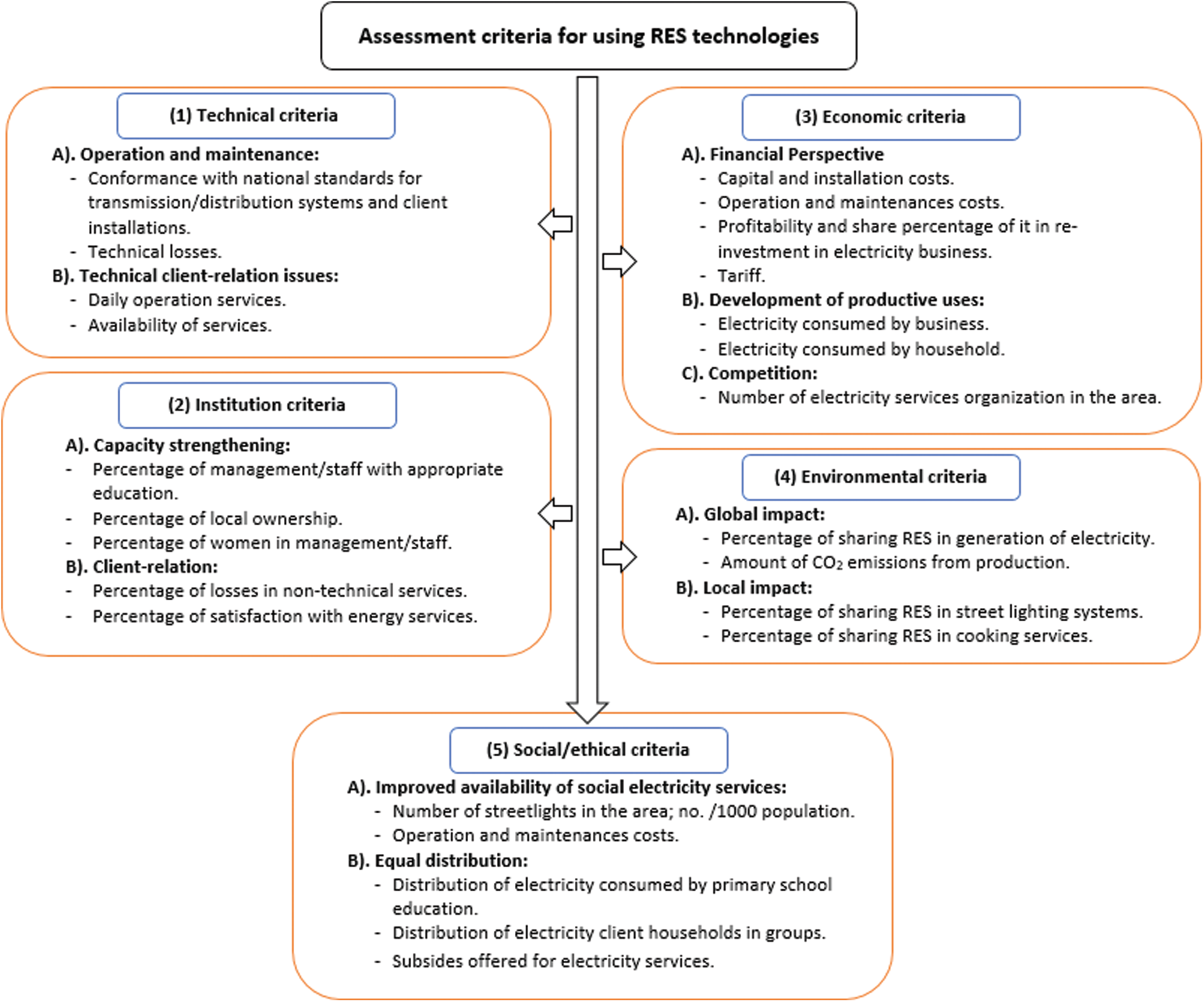
Figure 1: Assessment criteria for using RES technologies

The variety of available technologies and equipment to achieve specific goals is a characteristic feature of the modern era. The ratios of parameters such as price, performance, reliability, durability, safety, environmental friendliness, ergonomics, etc. constitute the issue of optimal choice. In a situation when there are 5–7 choices with immense object attributes and competing criteria; there is no obvious choice for the optimal solution.

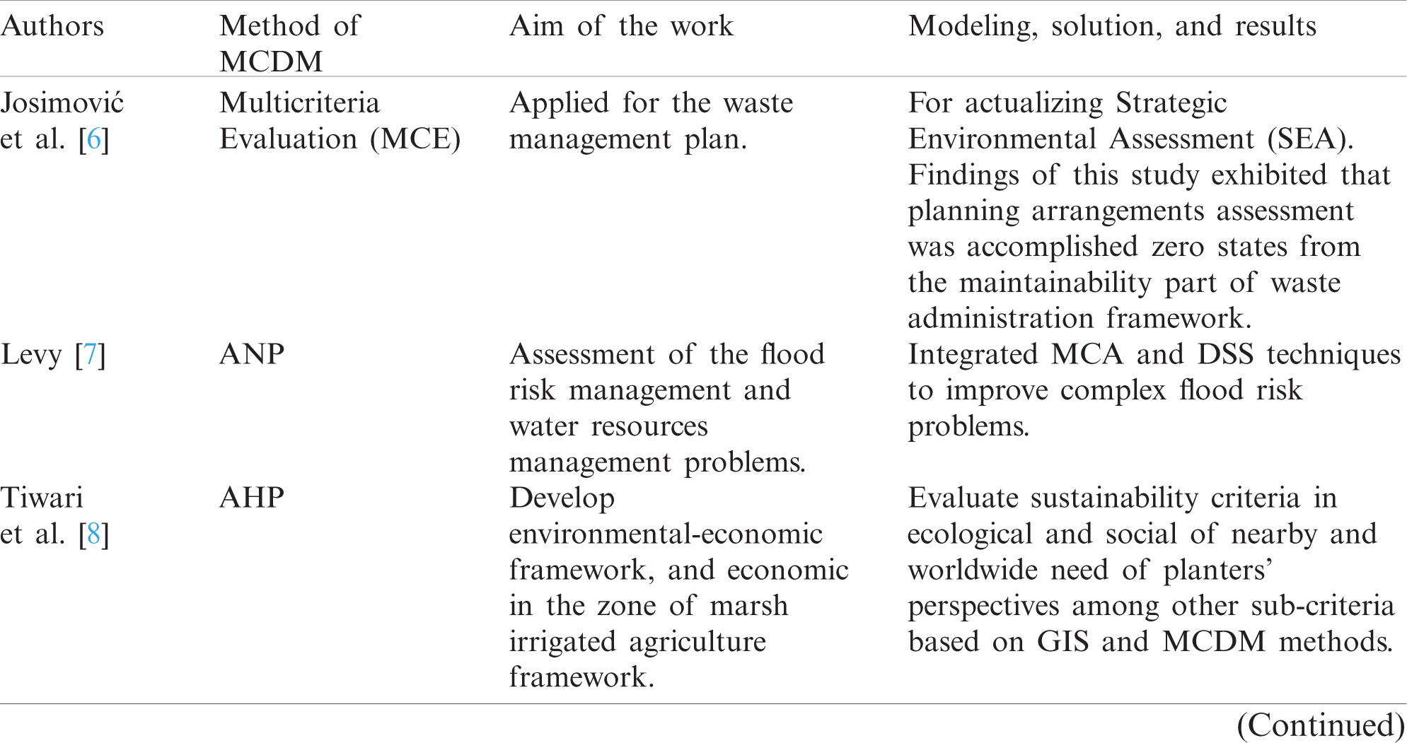
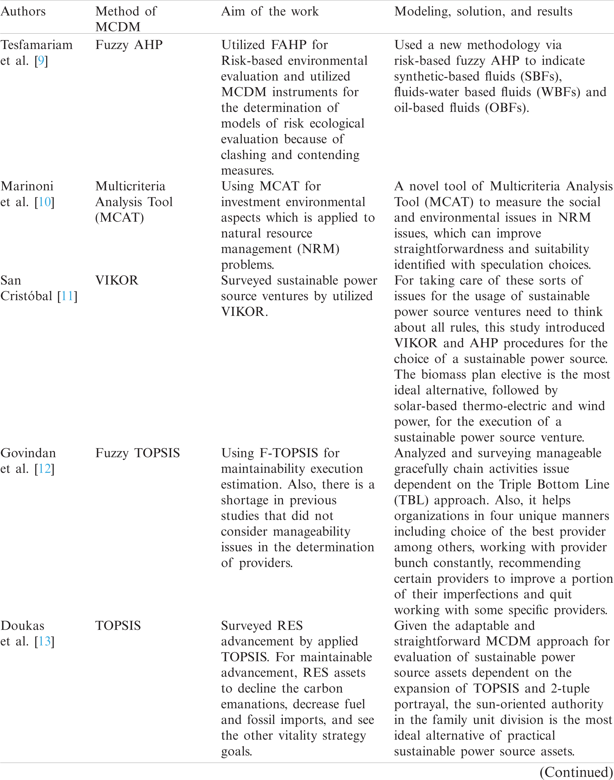
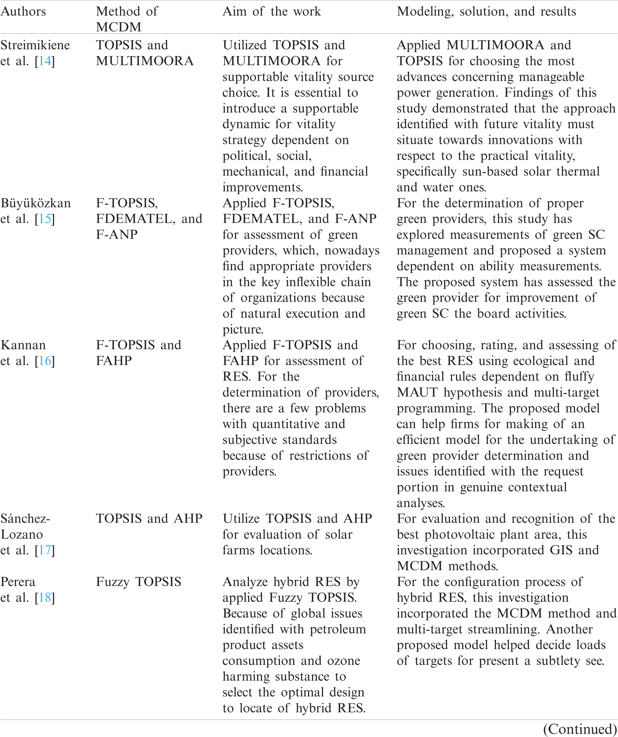
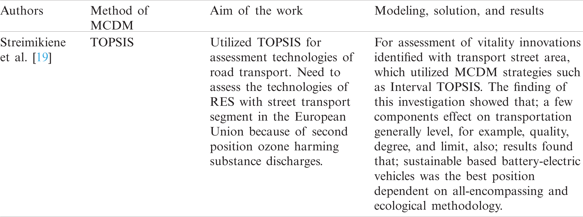
One of the approaches to solve this problem of optimal choice is the use of various multi-criteria solution techniques i.e., Multi-criteria decision-making (MCDM/MCDA) [3–5] and integration of methods into the engineered design process. Though, MCDM models are partially formalized and for them there is no concept of an absolute optimal solution. Nevertheless, as practice shows, MCDM models allow the selection of best option among predefined alternatives. If several alternatives have some of the attributes as “strong” and approximately the same part as “week,” then the performance indicators of such alternatives will differ significantly, and the alternatives will be hardly distinguishable. This requires a comprehensive analysis using various MCDM models and solution-based sensitivity analysis, where partially formalized quantitative (or qualitative) analysis is the basis for decision-making. Tab. 1 reviews the previous literature on MCDM methods showing aim of the work, modeling, solution, and main results of the literature work [6–19].

Table 1: Literature review’s summary

The main contributions of this research work can be summarized as:

1.    Based on multi-criteria decision-making models, implementing the integration of MCDM rank methods into the process of engineering design of hybrid renewable energy systems.

2.    Four different methods of weight estimation are considered for usage; no priority of criteria, criteria based on a pairwise comparisons matrix, CRITIC-method, and entropy-based method.

3.    A step-by-step methodology for forming various MCDM models and subsequent analysis of the results is described.

2  Description of the Case Study

The case study represents a flat 70 acres site in the Al-Minya city (Egypt) as an example of the far region location. The latitude and longitude is 28∘ N and 30∘ E, respectively. The nearest electrical grid point was 12 km from this location. The site is wealthy with solar irradiance. The mean solar irradiance level was 5.97 kWh/m2/day [20]. The maximum and minimum solar radiation values were 8.056 and 3.555 kWh/m2/day, respectively, for June and December. The sunshine period was about 9 to 11 h per day all year except for a few cloudy days. The hourly solar irradiance profile for every month is presented in Fig. 2.

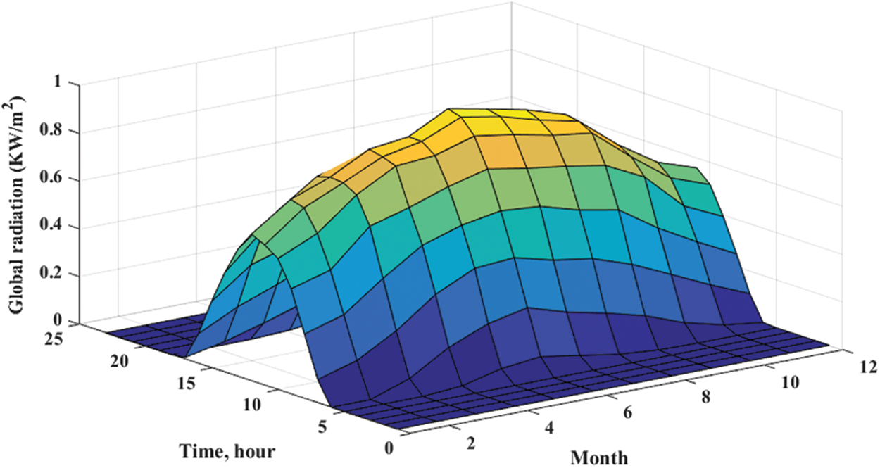
Figure 2: The solar irradiance profile for every month (kW/m2) per day, Al-Minya city (Egypt)

On the site, there was a well with the following specifications: 150 m depth, 40 m static level of water, 120 m3 the hourly rate of discharge. The salinity of brackish water was 2500 mg/l. It had been scheduled to cultivate part of the land with crops using the raw brackish water. The reminder was cultivated with Wheat as it cannot grow with brackish water. The salinity of the water needed to be lower than 800 mg/l. The amount of desalinated water was 250 m3/day. The required amounts of brackish water were 350–500 m3/day and 250–300 m3/day in the summer and winter periods, respectively.

The required energy to extract the brackish water was around 110 kWh/day with a peak of 15 kW. For desalination of the brackish water, it was scheduled to employ a reverse osmosis (RO) unit. Two different sizes of RO units, RO-250 and RO-500, were considered. The electrical peak demand values were 15 and 29.5 kW for RO-250 and RO-500 respectively [21]. To collect 250 m3, RO-250 operates 24 h every day. So, the total required energy was 360 kWh/day. While, to collect the same amount by RO-500, 12 h of operation was required with a total consumption of 354 kWh/day.

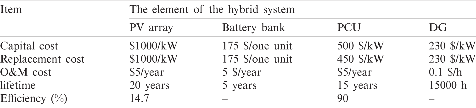
Fig. 3 illustrates the suggested hybrid system, which contains a Fixed PV array at a tilt angle of 28-degree, DG, power conditioning unit, and battery storage bank. The model of battery was Trojan L16P (360 Ah, 2.16 kWh). The input techno-economic specification data for different elements of a hybrid system are shown in Tab. 2 [22–24]. These data were used for determining the system’s best sizes using HOMER®; software [25,26]. Various options containing three different power sources: only DG, PV-B system, and hybrid PV-DG-B, two different sizes of reverse osmosis (RO) units; RO-250 and RO-500, two strategies of energy management; load following (LF) and cycle charging (CC), and two sizes of DG; 5 and 10 kW were taken into account. The optimal size of each option was selected based on the minim cost of energy.

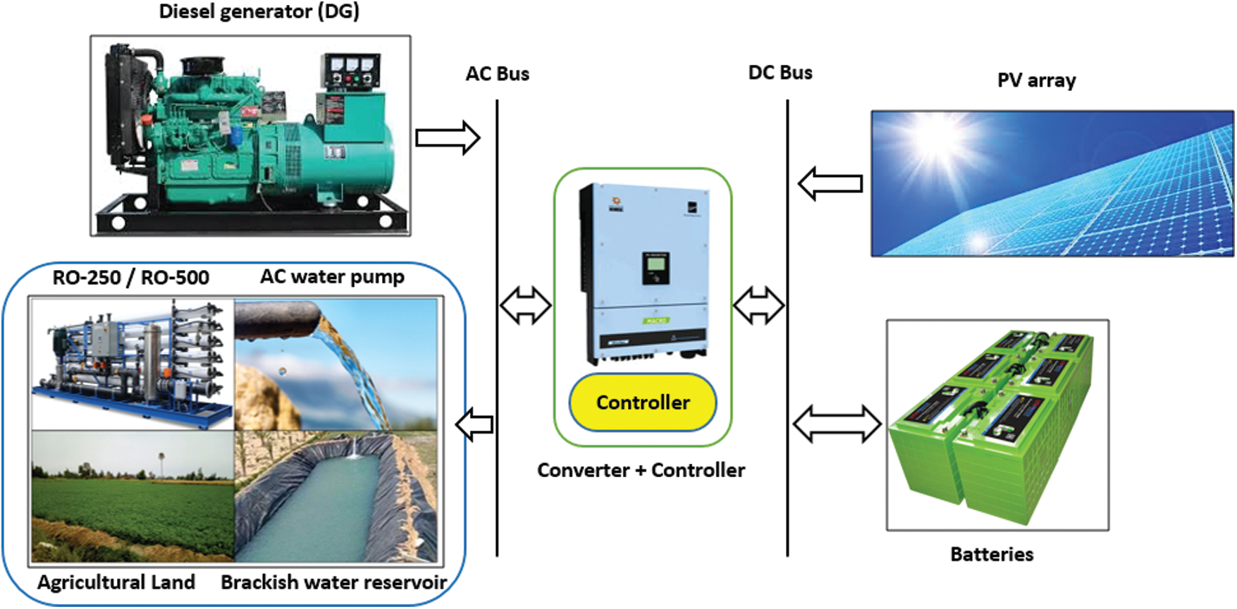
Figure 3: Renewable energy system (RES) schematic graph, Al-Minya city (Egypt)

Table 2: Specification of different elements of the hybrid system

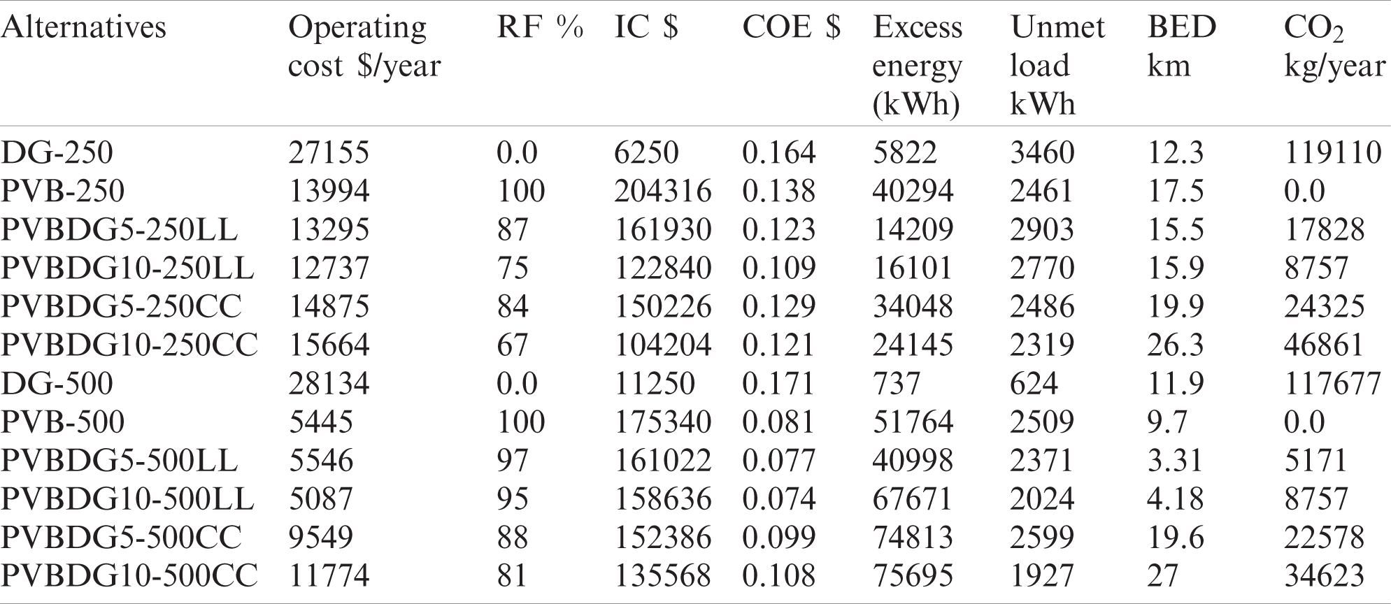
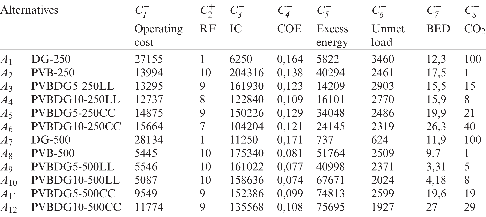
To identify the best option for the case study, MCDM tools were used. Eight parameters, including operating cost, renewable fraction, initial cost, the cost of energy, excess energy, unmet load, breakeven grid extension distance, and the amount of CO2 were considered during the determination of the best option. Tab. 3 shows the output of eight parameters for every considered option.

Table 3: The eight output parameters for all alternatives

3  Basic Methods and Formulas of MCDM

3.1 Aggregation Models

3.1.1 SAW (Simple Additive Weighting) Method [3–5]

Performance indicator Qi of the i-th alternative was determined as the entire standardized estimations of the attributes rij with the weight wj of the j-th criteria:

Qi=∑j=1nwj⋅rij,(1)

where; ∑j=1nwj=1 is the most elevated Qi score.

3.1.2 COPRAS (Complex Proportional Assessment) Method [27]

The aggregation method uses the construction of a performance indicator of alternatives based on the homogeneous function of the two arguments S+i and S−i:

Qi=S+i+(∑i=1mS-iS-i∑i=1m(1S-i)),(2)

where;

S+i=∑j=1nwj⋅rij∣forj∈Cj+,S-i=∑j=1nwj⋅rij∣forj∈Cj-,(3)

The above equation represents the sum of the normalized attribute values with weight revenue criteria and cost criteria. The best alternative was the one with the most elevated Qi score.

3.1.3 TOPSIS (Technique for Order of Preference by Similarity to Ideal Solution) [3]

To determine the performance indicator of the i-th alternative Qi, a homogeneous function was used:

Qi=Si-Si++Si-,(4)

where;

vij=rij⋅wj,Si+=d(vij,vj+),Si-=d(vij,vj-), (5)

vj+={maxivij|ifj∈Cj+;minivij|ifj∈Cj-}, (6)

vj-={minivij|ifj∈Cj+;maxivij|ifj∈Cj-}. (7)

Si+ and Si- were the distances d between the ideal and anti-ideal objects respectively. Whereas, the alternative Ai in the n-dimension attributes space, which are defined in one of the Lp-metrics (Section 3.2). The TOPSIS ranking result depends on the choice of distance metric. The best alternative was the one with the highest Qi score.

3.1.4 GRA (Gray Relation Analysis) [28]

It evaluates the effectiveness of alternatives in two groups with respect to ideal and anti-ideal objects. The sequence of calculations is as follows:

Step 1: Define two sets of attributes i.e., ideal and anti-ideal:

rj(1)={maxi(rij),ifj∈Cj+ mini(rij),ifj∈Cj-,rj(2)={mini(rij),ifj∈Cj+ maxi(rij),ifj∈Cj-,(8)

Step 2: Determine the matrix of deviations of normalized values from the ideal and anti-ideal:

Vij(1)=|rj(1)-rij|,Vij(2)=|rj(2)-rij|,(9)

Step 3: Determine the matrices the gray relational coefficient:

gij1=mini(minjVij1)+β⋅maxi(maxjVij1)Vij1+β⋅maxi(maxjVij1), (10)

gij2=mini(minjVij2)+β⋅maxi(maxjVij2)Vij2+β⋅maxi(maxjVij2). (11)

Step 4: Determination of the indicator performance for the alternative Qi:

Qi=Qi1/Qi2, (12)

Qi1=∑j=1ngij1⋅ωj,Qi2=∑j=1ngij2⋅ωj. (13)

Here, the best alternative was the one with the highest Qi score.

3.1.5 VIKOR (VIsekriterijumsko KOmpromisno Rangiranje) [29]

Step 1: Determination of “ideal” and “anti-ideal” object can be expressed as:

aj+={maxiaij|ifj∈Cj+;miniaij|ifj∈Cj-},aj-={minivij|ifj∈Cj+;maxivij|ifj∈Cj-},(14)

Step 2: Weighted normalization:

xij=ωj⋅aj+-aijaj+-aj-;(15)

Step 3: Maximal R and the group utility S strategies can be expressed as:

Si=∑i=1nxij;S*=miniSi;S*=maxiSi;Ri=maxixij;R*=miniSi;R-=maxiRi(16)

Step 4: Calculate the values of Qi:

Qi=v⋅(Si-S*S--S*)+(1-v)⋅(Ri-R*R--R*),(17)

Here, v assumes the part of balancing factor between the general advantage (S) and the maximum individual deviation (R). Smaller estimations of v accentuate bunch gain, while bigger qualities increased the weight controlled by singular deviations. “Voting by majority rule” (v > 0.5); or “by consensus” (for v = 0.5); or “with a veto” (for v<0.5).

Step 5: The aftereffect of the system is the three-rating records S, R, and Q. The options were assessed by arranging the estimations of S, R, and Q models of the base worth.

Step 6: As a compromise arrangement, option A1 was proposed, which was best assessed by Q (minimum) if the accompanying two conditions were met:

Condition C1: “Allowable advantage”:

Q(A2)-Q(A1)≥1(m-1),(18)

where; A2 is an alternative in contrast to the second situation in the Q ranking rundown:

Condition C2: “Adequate soundness in decision-making”: Alternative A1 ought to likewise be best assessed by S or/and R.

Step 7: If one of the conditions 1 or 2 was not fulfilled, a lot of negotiating arrangements were proposed, which comprises of:

Alternatives A1 and A2; if condition C2 is not met, or

Alternatives A1, A2,…,Ak; if condition C1 is not fulfilled. Where, Ak is controlled by the connection:

Q(Ak-1)-Q(A1)<1(m-1);Q(Ak)-Q(A1)≥1(m-1)(19)

3.1.6 PROMETHEE (Preference Ranking Organization Method for Enrichment Evaluations) [30]

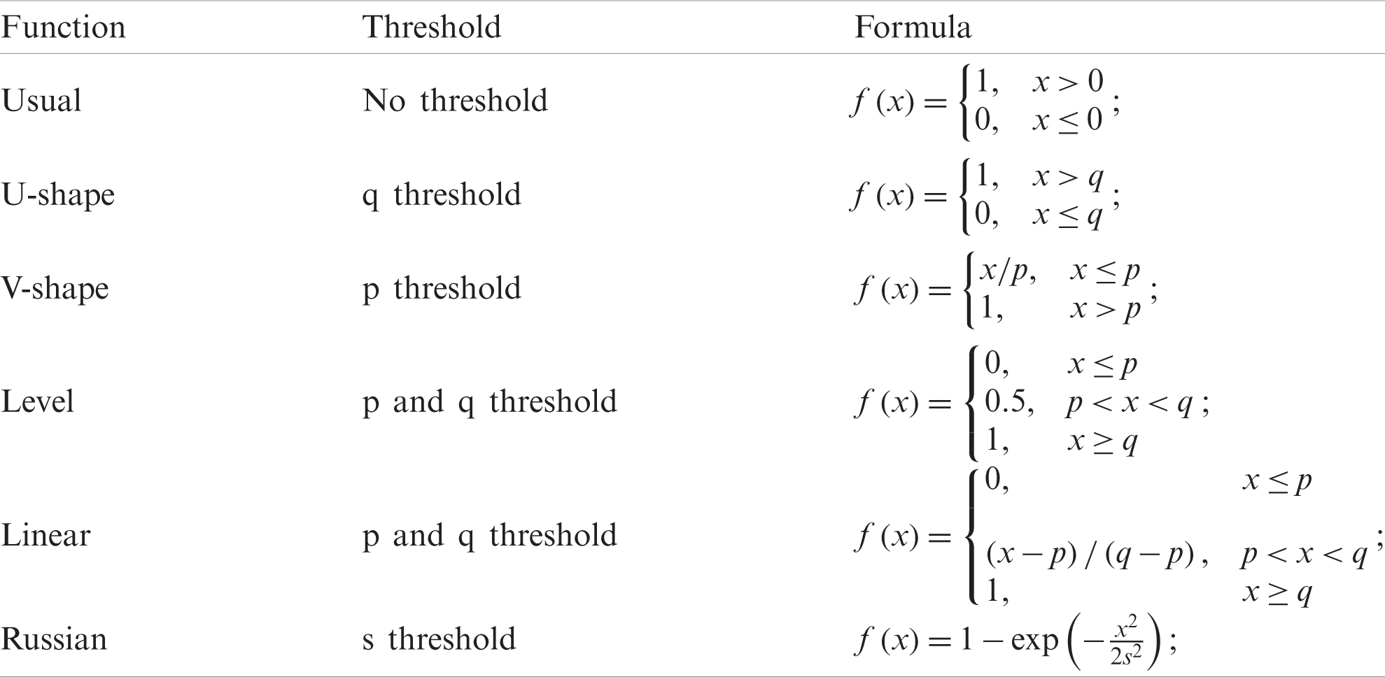
Step 1: Set the inclination work for two items for every model Hj = H (dis, p, q). When in doubt, they have two boundaries: p-indifference edge, it mirrors the way that if the distinction of these estimations of two options i and s are immaterial, objects by standard j were comparable. If the distinction in the limit esteem p was surpassed, an inclination connection was built up between the items. Similarly, if the distinction in edge q was surpassed, the inclination work, which compares the “strong preference” of variation i concerning s variation as for the j measure. With the distinction of dis in the stretch from p to q, the inclination work was under 1, which compares a “weak preference”. The decision of the inclination work was controlled by the leaders. A few sorts of capacities favored H(d) were introduced in Tab. 4.

Table 4: Preference functions for PROMETHEE-method

Step 2: Compute the distinction in the estimations of the models for the two items and calculate the inclination records V:

dis=aij-asj;Hj(dis,p,q);Vis=∑j=1nwj⋅Hj-[m×n]matrix(20)

Step 3: Determination of the preference factors:

Φi+=∑s=1,s≠imVis;Φi-=∑s=1,s≠imVsiQi=Φi+-Φi-(21)

The best option is the one with the most elevated Qi score.

3.1.7 ORESTE (Organization, Arrangement to Sinteze of Relational Data) [31]

Step 1: Change from network DM to ranks matrix (the columns of the matrix are supplanted by their ranks).

rij=rank(aij|{a1j,a2j,…,amj}),∀i,j(i=1,…,m;j=1,…,n).(22)

Step 2: Determine the ranks of criteria:

rcj=rank(Cj|{C1,C2,…,Cn}),∀j=1,…,n,orrcj=rank(wj|{w1,w2,…,wn}).(23)

Step 3: The projections of ranks were computed:

dij=[(1-α)⋅rijp-α⋅rcjp]1/p,α∈(0;1).(24)

p-one of: p = 1 Average (CityBlock, TaxiCab or Manhattan) distance,

p = 2 Mean Square (Euclidean) distance,

p=∞ Chebyshev distance.

Step 4: Calculating Ranks dij

Rdij=rank(dij|{dij}i=1:m;j=1:n),Ri=∑j=1nRdij.(25)

Step 5: Calculating Ranks Ri (ORESTE 1)

OutRi=rank(Ri|{R1,R2,…,Rm}).(26)

Step 6: Calculation of preference factors Cik

Cik=12⋅n2⋅(m-1)⋅∑j=1n(Rdij-Rdkj+|Rdij-Rdkj|). (27)

rij=jrank(aij);Rij=jsort(aij,‘descend’ifj∈Cj+ or ‘ascend’ifj∈Cj-) (28)

The best option was the one with the lowest Qi score.

3.2 Distance Metric

Distance metric was used to choose measurement to quantify the distance between two n-dimensional objects x and y:

Lp(x,y)=[∑j=1n(xj-yj)p]1/p,1≤p≤∞;L∞(x,y)= maxj|xj-yj|(29)

3.3 Normalization Methods

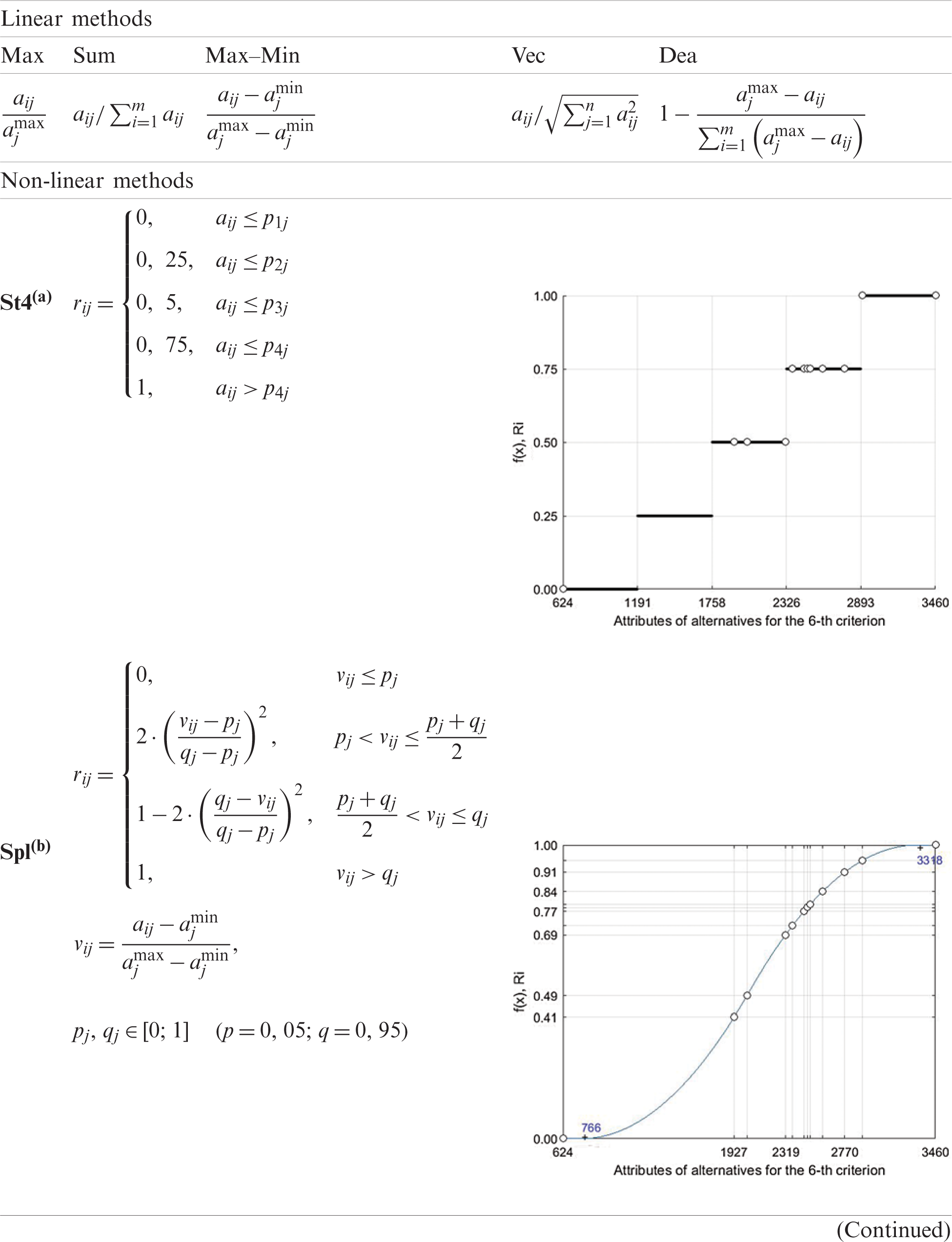
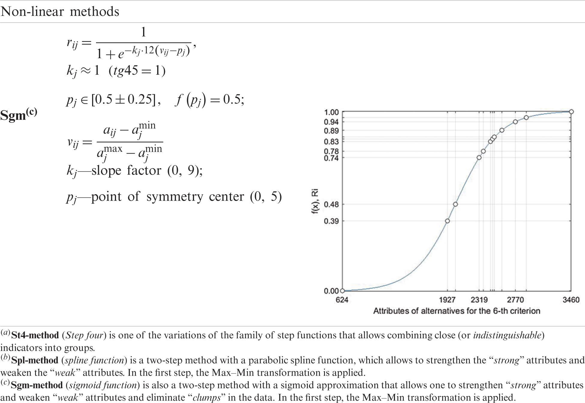
The study used the following 8-normalization methods [32,33] as listed in Tab. 5.

Table 5: The 8-normalization methods used in the study

3.4 Normalization for Cost Criteria

Two-Step Res-algorithm for inversion of cost credits into advantage ascribes [33]:

1)rij=Norm(aij),∀j=1,…,n2)r̃ij*=-rij*+rj*max+rj*min,∀j*∈Cj-.(30)

where; the linear normalization method Norm(aij) in the first step was applied to both, the benefit attributes and the cost attributes, and index j* meets the cost criteria.

3.5 Methods for Weight Estimation

3.5.1 No Priority of Criteria

wi=1/n(31)

3.5.2 Estimation the Weights Based on a Pairwise Comparisons Matrix of the Criteria [34]

Step 1: Determine pairwise comparison matrix P in T, Saaty scale.

Step 2: Determine eigenvector (v) for max eigenvalue λmax of matrix P (the calculations use the MATLAB function eigs( )):

[v,λmax]=eigs(P,1),(32)

Step 3: Calculate consistency index (C.I.) and compare with Tab. 5 of random consistency index (R.I.(n)).

C.I.=(λmax-n)/(n-1),(33)

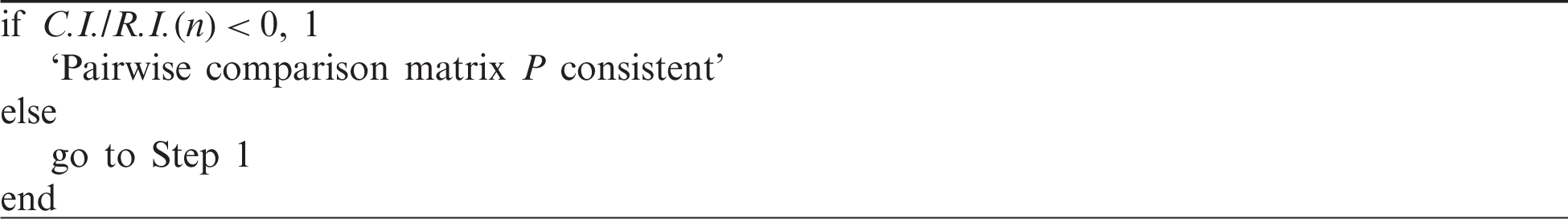
Step 4: Check the consistency of the pairwise comparison matrix. Compare the consistency index (C.I.) with the values of (R.I.(n)):

Step 5: Calculate weights of criteria:

wj=vj/∑j=1nvj(34)

In this case study, the values of the P were listed in Tab. 6.

Table 6: Values of the P-matrix in the case of study

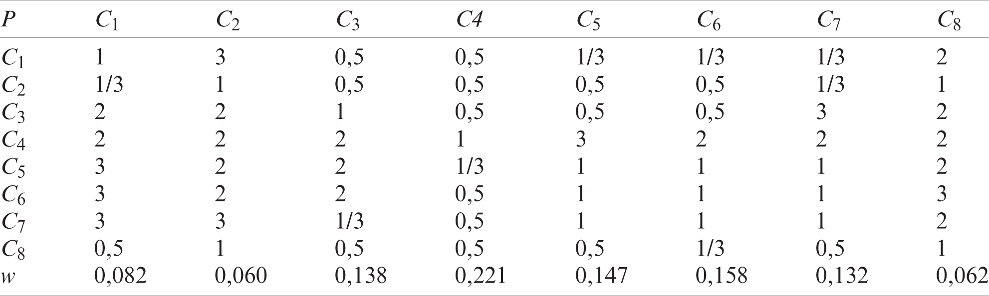
C.I./R.I.(n) = 0,07.

3.5.3 CRITIC-Method (Criteria Importance Through Intercriteria Correlation) for Weight Estimation [12]

Step 1: Determine ‘best’ (b) and ‘worst’ (t) solution ([1×n]-vector) for all attributes.

Step 2: Determine relative deviation matrix V = (vij) [m×n]-matrix

vij=(aij-bj)(bj-tj).(35)

Step 3: Determine standard deviation (St) ([1×n]-vector) for colls of V.

St=std(V)(36)

Step 4: Determine correlation matrix (Cr) ([n×n]) for colls of V.

Cr=corr(V)(37)

Step 5: Determine vector (c) and calculate the weight of criteria wk.

ck=Stk⋅∑j=1n(1-Crkj),k=1,…,nwk=ck/∑k=1nck.(38)

In this case study, the values of the B, T, and w were listed as:

b = [5087 10 6250 0,109 5822 2319 12,3 1],

t = [28134 1 204316 0,164 40294 3460 26,3 100], and

w = [0.104 0.124 0.166 0.102 0.175 0.100 0.111 0.119].

3.5.4 Entropy-Based Method for Weight Estimation [13]

The step-by-step algorithm for estimating the weights of the criteria using the entropy method was presented as follows:

Step 1: Standardized decision matrix (Max–Min method) for benefit criteria:

rij=aij-ajminajmax-ajmin,(39)

For cost criteria:

rij=ajmax-aijajmax-ajmin.(40)

Step 2: Calculate the equity contribution of the i-th attribute for each criterion:

fij=rij∑i=1mrij,∀i=1,…,m,j=1,…,n;∑i=1mfij=1,(41)

Step 3: Calculate the entropy of each criterion:

ej=-∑i=1mfij⋅ lnfij lnm,j=1,…,n;(ifrij=0⇒fij⋅ lnfij=0),(42)

Step 4: Calculate the weight of each criterion:

ωj=1-ejn-∑j=1nej,j=1,…,n,∑j=1nωj=1.(43)

The value (1 − ej) is the internal intensity of the contrast of each criterion or is the degree of divergence of the internal information of each criterion [35,36]. The smaller value of the entropy, the larger the entropy-based weight. In this case study, the values of the w were listed as:

w = [0,093 0,082 0,106 0,023 0,180 0,032 0,086 0,398].

4  MCDM Techniques

4.1 MCDM Rank Model

The ranking-based MCDM model for every elective Ai decides a specific exhibition level of the choices Qi based on the ranking of the other options, and the ensuing decision-making was obtained [3–5]:

Ai→FQi,i=1,…,m, (44)

Q=F(A,C,D,ω,‘nm’,‘dm’,‘pr’), (45)

Ap≺Aq≺…≺Ar≺As,p,q,r,s∈{1;2;…;m}. (46)

The MCDM rank model incorporates the decision of a lot of alternatives (A) and a set of criteria (C), an evaluation of the estimations of the characteristics of choices with respect to every criterion-a decision-making matrix (aij), a method for assessing the weight or priority of criteria (w), a choice of a normalization method (‘nm’) decision-making matrix, a choice of metric for calculating distances in n-dimensional space of criteria (‘dm’), a choice of preference functions (‘pr’), and the definition of aggregation function of alternatives’ attributes (F) to calculate efficiency indicator (Q) of each alternative. Based on the calculation of the aggregate performance indicator of alternatives Q, alternatives were ranked, i.e., SAW ranking model is simplified as:

Qi=∑j=1nwj⋅rij.(47)

where rij are the standardized estimations of the regular estimations of the qualities aij, acquired utilizing one of the standardization techniques. None of the arguments to F were unambiguous. The choice of A and C was not formalized, the estimates aij were not accurate, the choice of the method for evaluating the weights of the criteria, the method of the standardized method, the method of aggregation, and the choice of the distance metric were not formalized, as there were no selection criteria. Therefore, different combinations of 8 basic parameters in Eqs. (44)–(46) define different MCDM models.

4.2 MCDM Formalization of the Problem of Choosing Hybrid Renewable Energy Systems

In the present study, different models were defined by combining the ‘nm’ normalization method, the aggregation method F, the choice of different distance metrics, and different preference functions. Thus, for integration into the engineering design process of hybrid renewable energy systems, 55 models or variations of the basic ranked MCDM methods have been identified in Tab. 7.

Table 7: Constructor of alternative ranking models

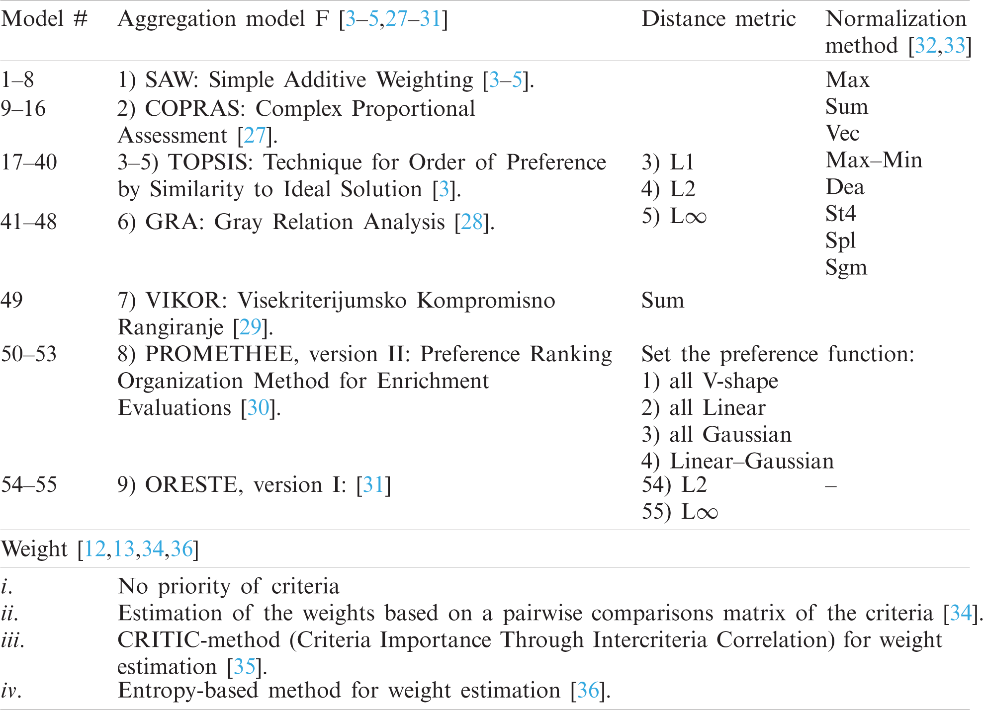
Combining 4 different methods for evaluating criteria weights, gives 220 options for ranking alternatives. Besides, the following model notation was used in the form of a cortege: # ={‘F’, ‘w’, ‘nm’, ‘dm’, ‘pr’}. For example, model #18 = {TOPSIS, (ii), Sum, L1} uses the TOPSIS attribute aggregation method, (ii)-a method for evaluating criteria weights, the Sum normalization method and the CityBlock-metric [3–5,27–31].

How much the ranking results differ depends on many factors. First, a ranking of alternatives was determined by the partial preference of various alternatives among themselves according to individual attributes. Suppose one of the alternatives has a preference over the other alternative according to several criteria, and vice versa, the other alternative dominates over the first according to another group of criteria. In that case, the performance indicators of these alternatives differ slightly. Although the aggregation methods, normalization methods, and the choice of parameters for preference functions affect the ranking result insignificantly, their small variations, together with a weak distinction of alternatives determine the ranking results [37]. Another parameter determining the ranking is the criterion weight. The weights directly determine the preference of alternatives over each other according to certain criteria. Therefore, the assessment of the criteria weights requires a justification of the chosen method and subsequent comparative analysis and correction of the weights of various criteria. Following this, one of the tasks of the study is to determine several best alternatives based on the analysis of the ranking results when varying the methods and parameters in the MCDM models.

4.3 Description of Alternatives and Attributes of Hybrid Renewable Energy Systems; Decision Matrix

Tab. 8 presents a matrix of decisions for the selected list of alternatives and their attributes.

Table 8: Matrix of decision D [12×8]

All criteria except the second (C2+) were “cost” criteria (Cj-). Therefore, to aggregate the attributes of benefit and cost jointly, the inversion of the normalized values was used through the ReS-algorithm [33]. The ReS-algorithm allows the same normalization method to be applied to both benefit and cost attributes and is effective for all normalization methods.

To determine the priority of alternatives, it was not enough to compare the absolute values of the efficiency indicator Qi. Attribute values may not be accurate due to many factors. For example, an attribute can be measured where the data source may be unreliable, there was error in measurement, the measurements for various alternatives were carried out using different methods, some attributes may be random values or determined by the values of intervals, etc. Thus, the value of the performance indicator was determined with an error of Qi±ΔQi, and the distinguishability of alternatives was determined by the error ΔQi.

In many cases, it was not possible to estimate the error. Then use the “a priori” or expert estimate, expressing it as a percentage. For example, as follows: the error in assessing the indicator of the alternative’s effectiveness was 5% of its value. Considering that alternatives were ranked according to their place in the ordered list of performance indicators, it was advisable to determine a relative indicator to assess the distinguishability of alternatives:

dQp=(Qp-Qp+1)/rng(Q)⋅100%,p=1,…,m-1.(48)

where; Qp is the value of the performance indicator corresponding to the p-rank alternative, rng(Q)=QI-Qm. Following Eq. (48), dQp represents the relative (given in the Q scale) increase or decrease in the efficiency indicator for an ordered list of alternatives. Afterward, two alternatives: the relative increase in dQ of which differ less than the value of the given a priori error, should be considered indistinguishable. The dQ indicator was used to assess the distinguishability of alternatives and to compare the results of aggregation performed by different methods.

4.4 Estimation of Weights of Criteria

Tab. 9 presents the criterion weights obtained using the 4-methods of estimation [12,13,34,36].

Table 9: Values of the weighting coefficients of the criteria obtained by using various methods

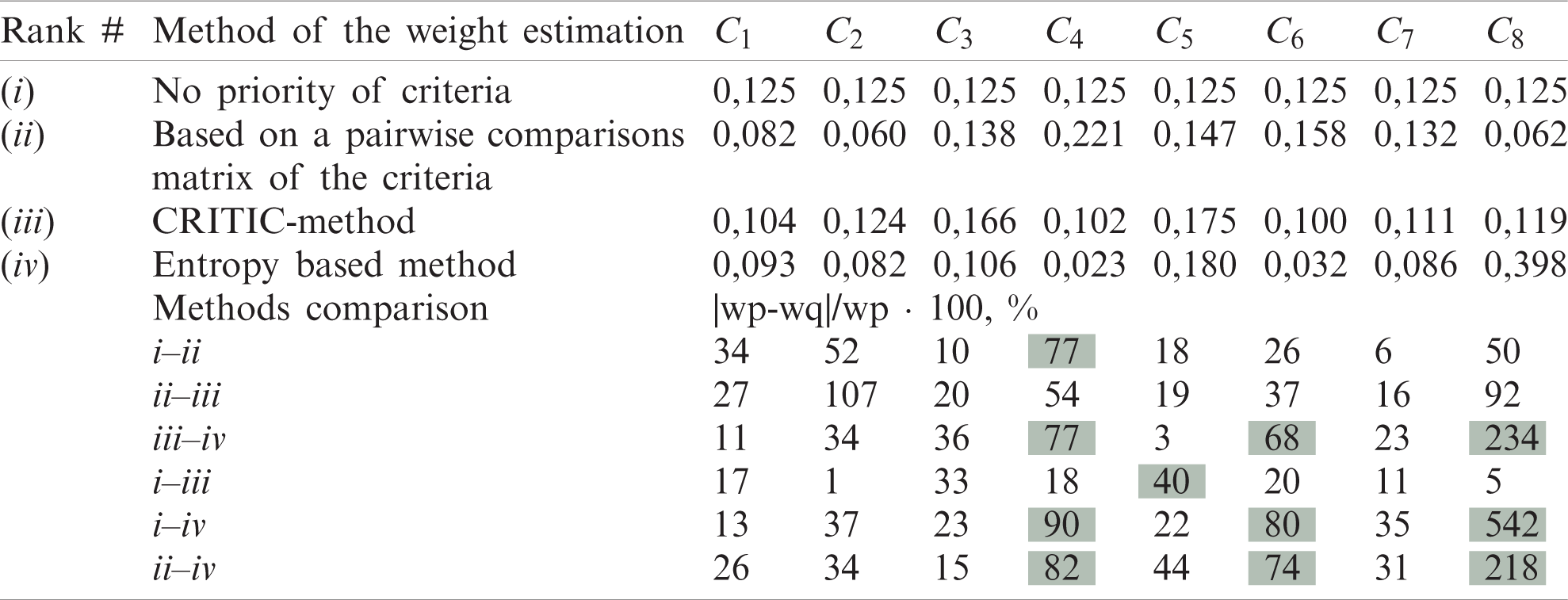
In the second part of Tab. 9, values of the relative difference (%) were given between the weights obtained by different methods. For the highlighted cells, the criteria weights differ significantly more than 70%.

For method (iv), the weight values for C8 were greatly overestimated (by 4–5 times) and the weight of C4 and C6 was greatly underestimated (by 4–5 times) in comparison with the weights determined by other methods. This overestimates the contribution of attribute 8 to the performance indicator of alternatives. It was expected that the priority 8 attribute alternatives will receive priority in the performance indicator. These are alternatives to A2, A8, A9, and A10.

The weights obtained using methods (ii) and (iii) differ on average by 30%. Both methods consider the relationship between different criteria in general, rather than the difference in attributes like the entropy-based method.

5  Results and Discussion

Calculations for various models were performed using the MCDM_tools software (version 2020), developed in the MATLAB system. MCDM_tools (version 2018) were posted in the public domain in a MathWorks File Exchange service on the website of the developer company MathWorks [38]. For each MCDM model, the performance indicator of each alternative Qi, the relative intensity iQ, the relative increment dQ were calculated and the ranks of the alternatives Ai were determined. An example of calculated indicators was presented in Tab. 9.

Tabs. 10, 11 present the synthetic results of ranking alternatives (based on Tab. 7) for various options (i)–(iv) estimates of the criterion weights obtained for 55 different MCDM models.

Table 10: Fragment of calculation results for the MCDM model #17–24 = {TOPSIS, (i), (Max, Sum, …, Sgm), L1,}

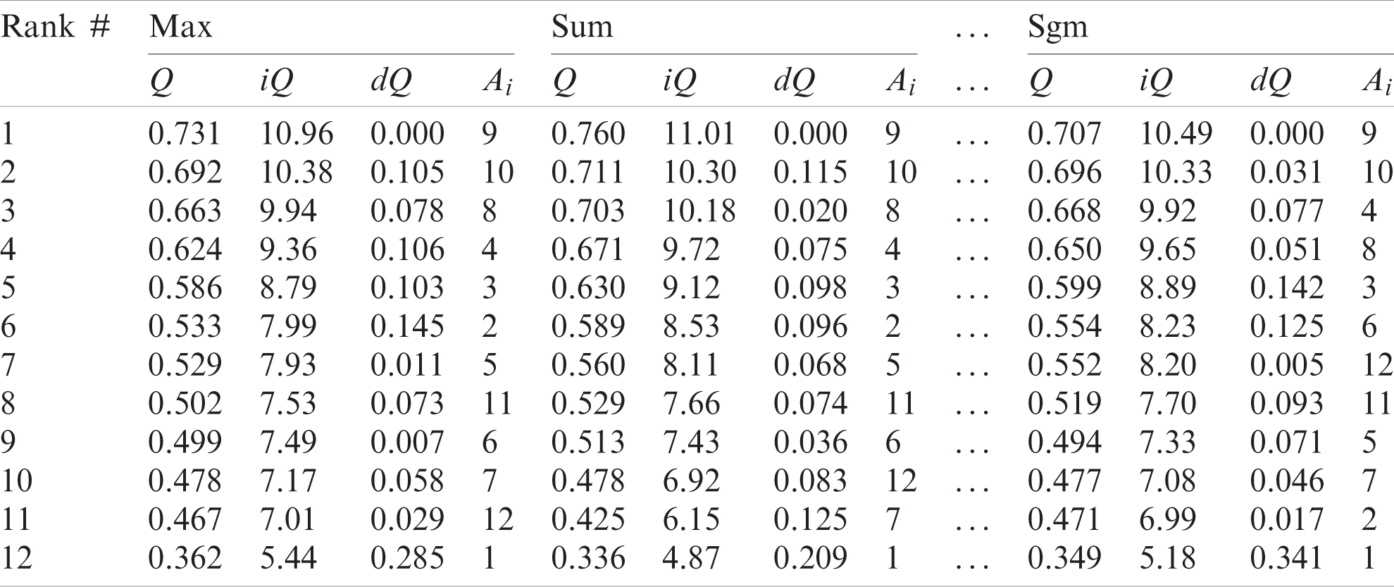
Table 11: Statistics of alternatives of I–III ranks based on the results of calculations of 55 MCDM models

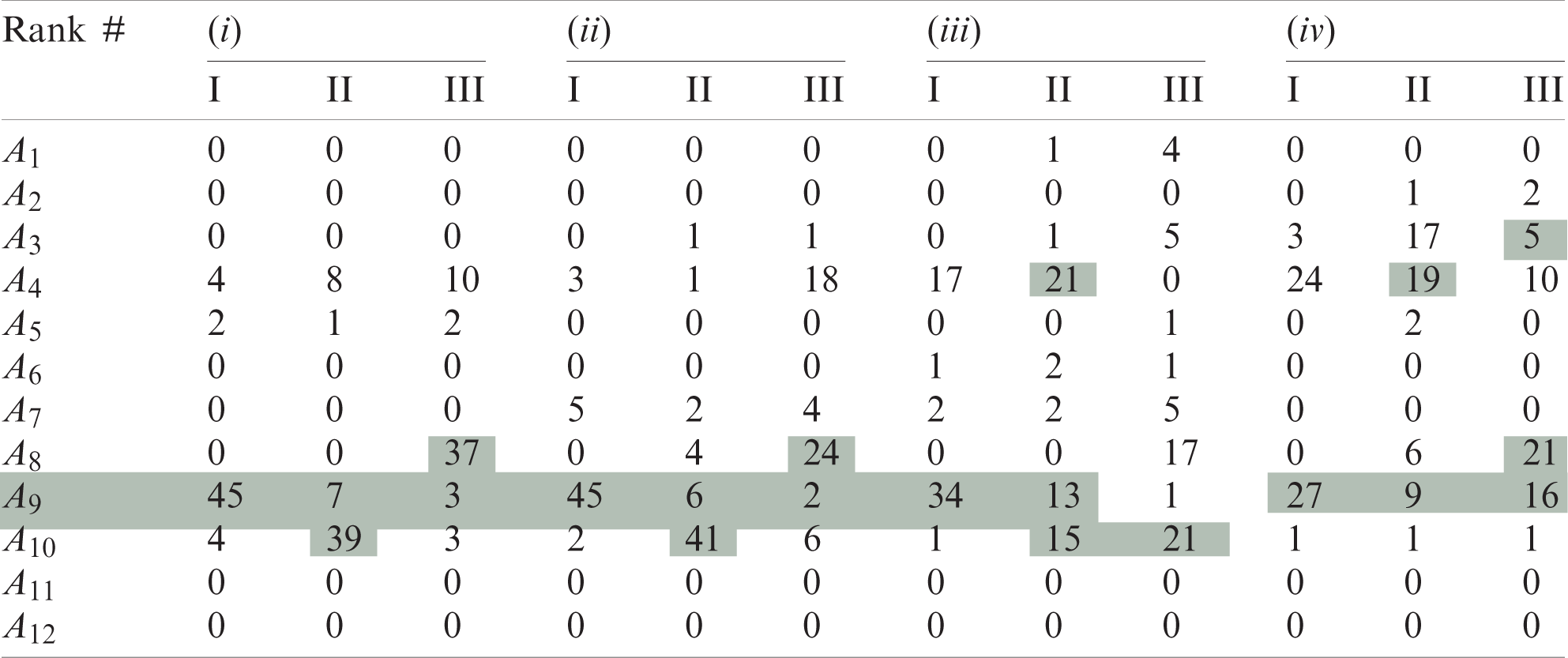
The numerical values in the Tab. 11 indicate how many times each of the alternatives A was ranked as I, II, III when ranks were based on 55 variants of MCDM models.

First: Let us consider the clearly “weak” alternatives that, according to the results of calculations, did not have high ranks. According to Tab. 8, it is A11 and A12.

Second: The assumption (Section 3.4) that, for the method (iv), all alternatives with a priority on attribute #8 will also receive priority in the performance indicator.

Indeed, according to Tab. 8 alternatives, A9 and A8 have I and II ranks in most models, and alternative A2 has II and III ranks in one and two cases, respectively, (and for other methods of estimating weights, I–III ranks are never achieved). The final ranks of the alternatives were presented in Tab. 12.

Table 12: Final rank of alternatives

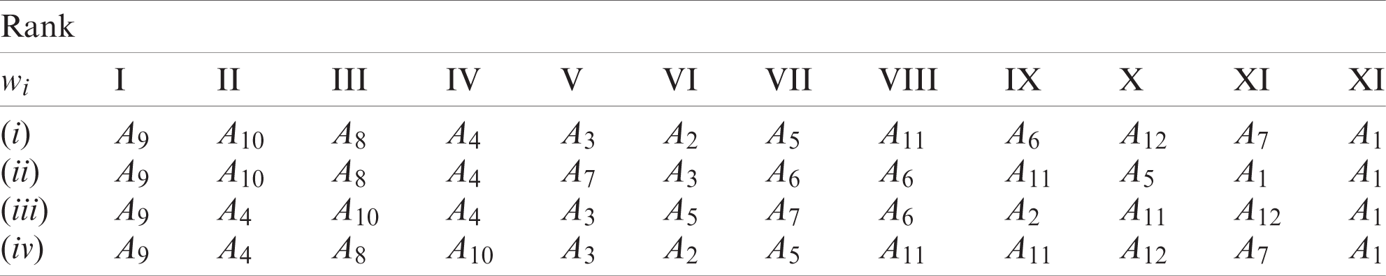
The unconditional leader was alternative A9. However, the alternatives A10, A7, A4, and A3 for some models (about 30% of variants) also had the first rank. Determining the leader by majority of votes cannot be a correct method. Additional information consists of assessing the distinguishability of alternatives using the relative performance indicators iQ and dQ.

Tab. 13 shows the ranks of alternatives (fragment) based on the results of calculations for 55 models in the case of determining the weights of the criteria by method (iii).

Table 13: Ranks of alternatives based on the results of 55 models in the case of determining the weights of criteria by method (iii) (Fragment)

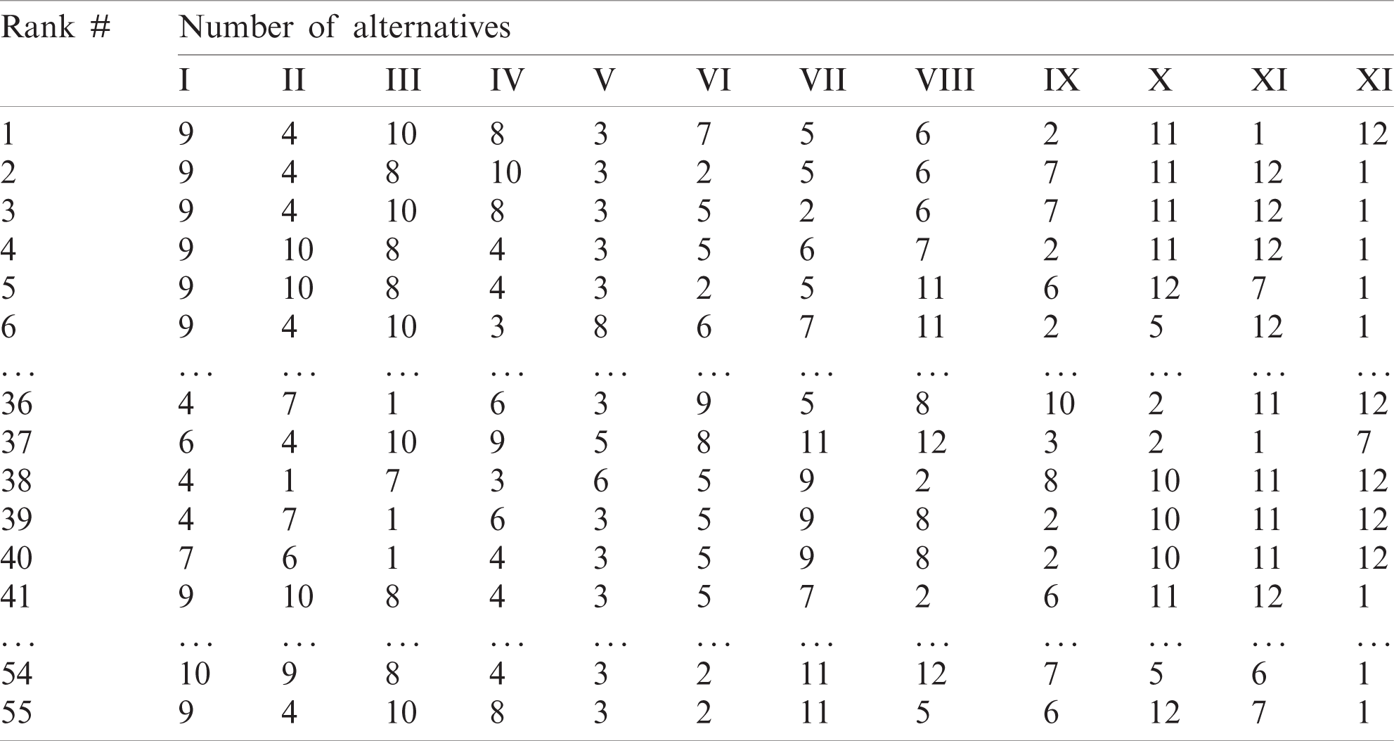
Tab. 13 and the data in Tab. 7 make it possible to select models for subsequent refinement of the leader. The specificity of MCDM models shows that for some models (more precisely, an unsuccessful combination of model parameters), a result is possible in which an alternative “weak” in terms of characteristics has a high rating (rank). For example, the alternative A1 has shown II rank in the model #38={TOPSIS,(iii),St4,L∞}, Tab. 11. In the absence of formal criteria for the selection of models, acceptance or rejection was possible if there were additional arguments (reasons).

Fig. 4 shows various histograms of the ranks of alternatives based on the results of calculations in 55 models (option (ii)). Data were collected in separate histograms considering the distinguishability of rank I–III alternatives.

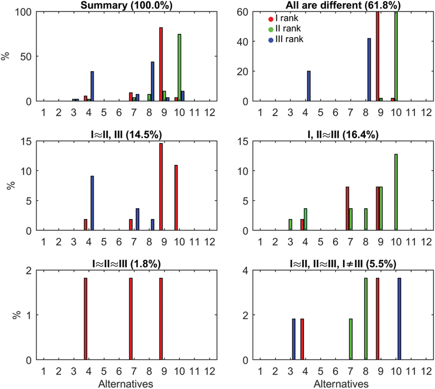
Figure 4: Distinguishability of the alternatives of rank I–III for (ii)-method

Fig. 5 shows the intensity of the performance indicator of alternatives of I–III ranks (points), considering their distinguishability for various models of aggregation of attributes. The results were collected in sequential groups corresponding to the eight different normalization methods as indicated in Tab. 2 (Model Builder)-{‘Max,’ ‘Sum,’ ‘Vec,’ ‘Max–Min,’ ‘Dea,’ ‘St4,’ ‘Spl,’ ‘Sgm.’} Colored markers illustrate the distinguishability of rank I–III alternatives.

Similar Figs. 4 and 5 were obtained for all the variants for evaluating the weights of criteria (i)–(iv). Tab. 14 presents a summary of the results.

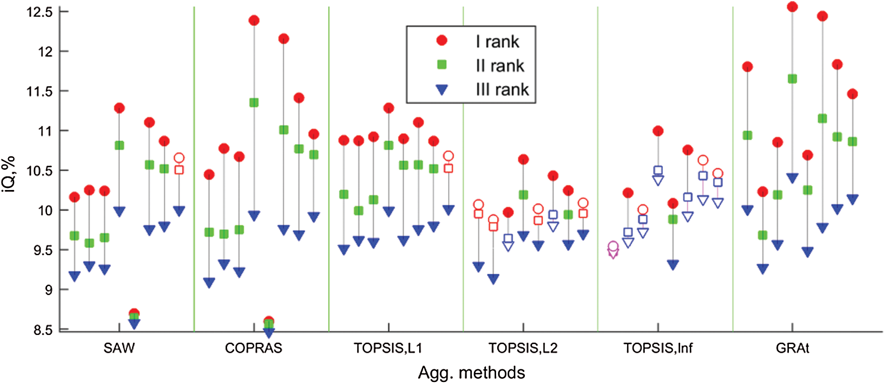
Figure 5: Distinguishability of the alternatives of rank I–III for the ii-method of weight estimation and linear normalization method

Table 14: Distinguishability of rank I–III alternatives; statistics for 55 models

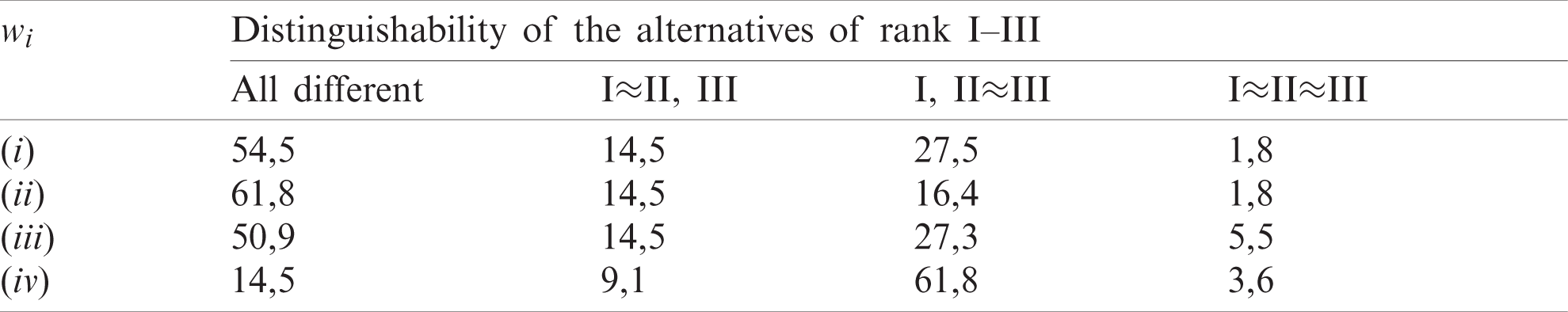
The distinguishability of alternatives of I–III ranks was no more than 61.8%, and the indifference of alternatives I, II, and III ranks above 30% cannot be made unambiguously. Alternatives A9, A10, A8, and A4 were recommended as suboptimal. The final decision was made by the decision-maker.

6  Conclusion

Based on various multi-criteria decision-making (MCDM) models, the best electrical energy source has been identified to feed both the water pumping system and the water desalination unit, respectively. The electrical energy source alternatives were suggested to consider different sizes of water desalination units, different energy management strategies, different sizes of diesel generators, and different system configurations. Four different methods of the weight estimation were considered; no priority of criteria, based on a pairwise comparisons matrix of the criteria, CRITIC-method, and entropy-based method. The results revealed that the best/optimal alternative of hybrid PV-DG-B consists of 5 kW DG, RO-500, and load following control strategy. The yearly operating cost and initial cost for such a system were $ 5546 and $ 161022, respectively, while the cost of energy was 0.077 $/kWh. The excess energy and unmet loads were 40998 and 2371 kWh, respectively. The breakeven grid extension distance and the amount of CO2 were 3.31 km and 5171 kg per year. Compared with DG only, the amount of CO2 has been sharply reduced by 113939 kg per year.

Funding Statement: The authors received no specific funding for this study.

Conflicts of Interest: The authors declare that they have no conflicts of interest to report regarding the present study.

This work is licensed under a Creative Commons Attribution 4.0 International License, which permits unrestricted use, distribution, and reproduction in any medium, provided the original work is properly cited.